Identification and Application of the Aerodynamic Admittance Functions of a Double-Deck Truss Girder

Abstract

This paper presents the aerodynamic admittance functions (AAFs) of a double-deck truss girder (DDTG) under turbulent flows. The objective of the investigation is to identify AAFs using a segment model wind tunnel test. All of the wind tunnel tests were based on the force measurement method and conducted in a passive spire-generated turbulent flow. The segment model adopts a typical DDTG section and is tested in the service and construction stages under 0°, 3°, and 5° wind attack angles. Furthermore, a nonlinear expression is put forward to fit the identified AAFs. The buffeting responses of a long-span road-rail cable-stayed bridge are then calculated for both the service and construction stages using an equivalent ‘fish-bone’ finite element model of the DDTG. The unsteady effect of the buffeting force is considered based on quasi-steady buffeting theory using the identified AAFs. The calculated buffeting responses are finally compared with those for two other AAFs (AAF = 1.0 and the Sears function). The results indicate that the traditional AAFs overestimate vibrations in the vertical and torsional directions but underestimate vibrations in the lateral direction. The identified AAFs of the DDTG can be regarded as a reference for wind-resistant designs with similar girder sections.

1. Introduction

To meet the stricter requirement for girder rigidity in railways and noninterference between rail and road traffic in China, truss girders are becoming more commonly applied in the design of long-span cable-stayed bridges, combining roadways and railways with double decks over 30 m in width [1]. When the truss girder length exceeds 1,000 m, the girder stiffness becomes lower, and the bridge flexibility becomes higher. Additionally, the first natural frequency is approximately 0.1 Hz or even lower. When built in wind-prone regions, these bridges suffer considerable buffeting-induced vibration. The buffeting-induced vibration occurs over a wide range of wind speeds and persists throughout the entire design life of the bridge. As a result, buffeting plays the most important role in the wind-resistant design of long-span cable-stayed bridges with double-deck truss girders (DDTGs).

The interaction of buffeting and wind is regarded as a significant excitation in flexible long-span bridges due to the low frequencies that characterize both the turbulence input and the structure. The aerodynamic admittance function (AAF) is one of the most important factors in evaluating the buffeting responses of slender, link-like structures, such as long-span cable-stayed bridges, in turbulent flows. The AAF is a transfer function from wind turbulence energy to fluctuating buffeting forces on structures. The AAF can take into account the unsteadiness of gust loading in a linear time-invariant system. In the 1900s, the AAF was derived from the aerofoil lift force studied by some scholars. Based on the strip assumption, the spanwise correlation of the buffeting force on structures could be displaced by the lateral correlation of turbulence. In 1941, Sears [2] was the first to propose a complete 2-dimensional lift AAF of a thin aerofoil immersed in a transversely fully coherent sinusoidal gust. As the milestone of AAF, this transfer function has been named the Sears function and applied in many studies as the 2D AAF of streamlined objects in turbulence. Following Sears’ approach, Liepmann [3,4] used statistical concepts to develop a buffeting analysis method for aerofoils in the frequency domain and obtained an approximate expression for the Sears function. Graham [5,6] gave the aerodynamic transfer function for the lift force on a thin aerofoil with infinite span by a numerical method. Moreover, some scholars (Filotas [7,8] and Mugridge [9]) put forward an approximate expression of the admittance for an aerofoil. However, all of these theorized admittance expressions were not derived for bluff bodies, and their universality is questionable. In recent years, some new developments have been made regarding the aerofoil admittance in parameter analysis, but most of these developments have been limited to streamline bodies [10,11].

For bluff bodies, such as a bridge girder section, the exact expression of the admittance cannot be theoretically derived like that for aerofoils due to their much more complex aerodynamic force caused by the separation and reattachment of flow. Jancauskas and Melbourne [12] measured the AAFs of 2D rectangular sections in smooth flow using a gust generation technique. They found that the Sears function underestimates the 2D AAF of these simplest bluff bodies. Therefore, the aerodynamic admittance of bluff bodies has mainly been determined based on wind tunnel tests. The experimental methods used to identify the AAF mainly consist of random response measurements on aeroelastic models and direct buffeting force/pressure measurements on rigid segment models. Based on the assumption that the Sears function could be expressed by the Wagner function or Theodorsen functions, some studies [13,14,15,16] obtained the admittance functions of bluff bodies with non-strict adaptability using the former methods. Considering convenience and practicability, a widely used experimental method is the wind tunnel test, which consists of surface pressure tube measurements and direct force measurements. Larose and Mann [17] proposed an empirical AAF model and spanwise coherence of the aerodynamic forces applied on a series of streamlined bridge deck cross sections through measurement of the unsteady surface pressures on a closed box girder under turbulence. Zhu et al. [18] identified six-component AAFs of a closed box based on a common force and pressure measurement test in passive grid-generated turbulent flow.

For truss girders, studies focused on the AAF are relatively few and have no universality due to the various geometric details. Larose [19] directly measured the admittance of a truss girder in a wind tunnel test. Sato [20] gave the admittance of a stiffening truss girder of the Akashi Kaikyo Bridge. Yingzi Zhong (2018) directly identified a truss girder’s aerodynamic lift admittance using buffeting force measurements based on the assumption that the truss girder is equivalent to a continuous cross-section girder. However, all of the studied truss sections had a single deck and were only used in long-span road bridges.

To date, research on the AAFs for DDTGs applied in long-span cable-stayed road-rail bridges has not been carried out. To overcome this deficiency, a series of wind tunnel tests were performed to identify the AAFs of a DDTG segment model based on a force measurement test in a passive spire-generated turbulent flow. In Section 2, the AAF identification approach is proposed theoretically. Section 3 gives a detailed introduction on the wind tunnel test. Section 3.1 describes the construction and installation of the test model. The test conditions are shown in Section 3.2. The turbulent wind flow characteristic in the wind tunnel and comparison with the target spectrum are studied in Section 3.3. In Section 4, the test results of AAFs are provided and fitted based on a combination of the common formula and an extremum expression. The identified AAFs are compared with the Sears function in terms of each component under the service and construction stages in Section 4.2. Finally, in Section 5, the buffeting responses for three AAF types (AAF = 1.0, the Sears function, and the identified AAFs) are discussed. All symbols used are listed in

Table 1. List of symbols.

U	Mean velocity of turbulence
B, H, L	Width, height and length of segment model
z	Relative elevation of DDTG
u, v, w	Velocity components of turbulence
α	Wind attack angle
FD, FL, FM	Measured drag force, lift force and pitch moment
CD, CL, CM	Drag, lift and pitch moment coefficients
$C_D^{\prime }$,$C_L^{\prime }$,$C_M^{\prime }$	Derivatives of drag, lift and pitch moment coefficients
Su, Sw	Power spectra of velocity components in the u and w directions
SD, SL, SM	Power spectra of drag, lift and pitch moment
Ixx, Iyy, Izz	Inertia moments of an equivalent girder

.

2. Aerodynamic Admittance Identification Methodology

Although buffeting forces are essentially unsteady, they are conventionally modelled based on quasi-steady theory and then modified by AAFs to consider unsteady behaviours [21,22,23]. Much research has shown that the average buffeting force remains constant, but the fluctuating aerodynamic force caused by turbulent wind is dependent on the dimensionless reduced frequency. Because the normal wind case is generally considered for most periods of bridge service, the AAFs related to the drag force (D_b), lift force (L_b) and pitch moment (M_b) are focused on and investigated most often, which was also done in this paper. According to Davenport [24], the buffeting force is often expressed by six AAFs:

$$D_b(x,t)=\frac{1}{2}\rho U^{2}B\left[2C_D\frac{u(x,t)}{U}{\chi }_{Du}^{}(t)+C_D^{\prime }\frac{w(x,t)}{U}{\chi }_{Dw}^{}(t)\right]$$

(1)

$$L_b(x,t)=\frac{1}{2}\rho U^{2}B\left[2C_L\frac{u(x,t)}{U}{\chi }_{Lu}^{}(t)+(C_L^{\prime }+C_D^{})\frac{w(x,t)}{U}{\chi }_{Lw}^{}(t)\right]$$

(2)

$$M_b(x,t)=\frac{1}{2}\rho U^2{B}^2\left[2C_M\frac{u(x,t)}{U}{\chi }_{Mu}^{}(t)+C_M^{\prime }\frac{w(x,t)}{U}{\chi }_{Mw}^{}(t)\right]$$

(3)

where ${\chi }_{ij}(t)$ (i = D, L, or M, corresponding to the lateral, lift and pitch moment loads, respectively, and j represents u or w, the wind direction components) is the component of the aerodynamic admittance of the buffeting loads in the respective wind direction.

Based on the frequency dependence of ${\chi }_{ij}(t)$, Equations (1)–(3) are transformed by the Fourier transform while neglecting the effect of cross spectra, and the sectional buffeting force spectra are expressed as

$$S_D(\omega )={\left(\frac{\rho UB}{2}\right)}^2\left[4C_D^2{S}_u(\omega ){\left|{\chi }_{Du}^{}(\omega )\right|}^2+C_D^{\prime }{}^2{S}_w(\omega ){\left|{\chi }_{Dw}^{}(\omega )\right|}^2\right]$$

(4)

$$S_L(\omega )={\left(\frac{\rho UB}{2}\right)}^2\left[4C_L^2{S}_u(\omega ){\left|{\chi }_{Lu}^{}(\omega )\right|}^2+{(C_L^{\prime }+C_D)}^2{S}_w(\omega ){\left|{\chi }_{Lw}^{}(\omega )\right|}^2\right]$$

(5)

$$S_M(\omega )={\left(\frac{\rho U{B}^2}{2}\right)}^2\left[4C_M^2{S}_u(\omega ){\left|{\chi }_{Mu}(\omega )\right|}^2+C_M^{\prime }{}^2{S}_w(\omega ){\left|{\chi }_{Mw}(\omega )\right|}^2\right]$$

(6)

Usually, the equivalent AAF method, or the autospectral method, is applied to identify the AAF for a bridge segment model based on fluctuating aerodynamic force and fluctuating wind velocity [16,19,25]. This method assumes that two AAFs (${\chi }_{iu},{\chi }_{iw},i=D,L,M$) in each S_i related to the same force component and wind velocities along u and w are equal to each other, i.e.,${\chi }_{iu}={\chi }_{iw}={\chi }_i$. In the frequency domain, this method can obtain the modulus squared value of equivalent AAFs for each force, i.e., ${\left|{\chi }_i\right|}^2$, which can ensure that the reproduced force auto spectrum is equivalent to the real or tested force autospectrum. ${\left|{\chi }_i\right|}^2$ is a weighted average of ${\left|{\chi }_{iu}\right|}^2$ and ${\left|{\chi }_{iw}\right|}^2$, and is often close to ${\left|{\chi }_{Dw}\right|}^2$, ${\left|{\chi }_{Lw}\right|}^2$ or ${\left|{\chi }_{Lw}\right|}^2$ for common bridges because the weight factors of these three AAFs in the spectral equations are often much larger than those of the other AAFs [18]. Then, for example, the AAF for the lift buffeting force can be expressed as

$${\left|{\chi }_L^{}(\omega )\right|}^2=\frac{S_L(\omega )}{{\left(\frac{\rho UB}{2}\right)}^2\left[4C_L^2{S}_u(\omega )+{(C_L^{\prime }+C_D)}^2{S}_w(\omega )\right]}$$

(7)

3. Experiment and Turbulent Wind Generation

Experiments were conducted in the BJ-1 wind tunnel located at Beijing Jiaotong University in Beijing, China. This tunnel is a closed-circuit-type wind tunnel with a high speed test section configuration of 2.0 m in height, 3.0 m in width, and 15 m in length. In the test section, the wind speed can be adjusted from 2 m/s to 40 m/s. The turbulence intensity in the empty tunnel is less than 1.0%.

3.1. Segment Model

To investigate the aerodynamic admittance of a DDTG, a typical steel-truss girder used in roadway-railway bridges was modelled in the current study. A 15-unit segment was selected to identify the AAFs. The size of the real girder was 35 m wide and 16 m high (Figure 1). This girder consisted of a top lateral bracing system for road traffic, a bottom box structure for railway traffic and three vertical oblique web members. The top lateral bracing was composed of an orthotropic bridge deck, cross beams, cross ribs, and cross links. The cross ribs and cross beams were both equidistantly distributed at 2.8 m under the road deck. In the cross section with vertical web members, a truss cross link was set between two adjacent vertical web members to increase the torsional stiffness of the truss structure. The bottom box deck serviced for four railway tracks and consisted of an orthotropic deck and cross ribs.

In the wind tunnel test, a geometric scale of 1:80 was selected for physical modelling of this kind of girder. Some factors of the segment model were taken into account to conform to the model scale ratio, including the geometric size of the truss girder bridge, model stiffness and configuration of the test segment. The blockage ratio of the wind tunnel test must be less than 5% to avoid influencing the test results. The dimensions of the high speed test section were 3.0 m (width) × 2.0 m (height), and the blockage ratio of the 1:80-scaled models in this study could reach up to 4.6%. The lengths of the real truss girder and the 1:80-scaled segment model were 210 and 2.625 m, respectively. The ventilation rate was 58%, similar to that of the real truss girder, and the height and width of the segment model were 0.223 m and 0.45 m, respectively. The test segment model was constructed with strict geometric similarity in some details, such as the U rib of the road deck, bar section, cross beams and cross ribs. Considering the strength and stiffness of the model, the framework of the main girder was made of lightweight stainless steel, obtained by argon arc welding. Other components, such as the roadway and railway decks, cross ribs and cross links, were made of ABS (Acrylonitrile Butadiene Styrene) plastic. The scaled models used in the wind tunnel test are shown in Figure 2.

3.2. Test Conditions

Considering that the buffeting response appears at different stages and wind attack angles, two main types of test were performed in our study:

• The service and construction stage test: the segment model was assembled with and without attachment to simulate the service and construction stages, respectively. The attachment could affect the geometric profile of the entire truss girder, with obvious changes in the aerostatic and aerodynamic characteristics of the segment model. The difference between these two stages is shown in Figure 3.
• The wind attack angle effect test: the segment model in the service stage was tested at wind attack angles α of 0°, 3° and 5°. The wind attack angle α is defined as the angle between the incoming wind direction and the segment model, adjusted by an α holder independent of the wind tunnel.

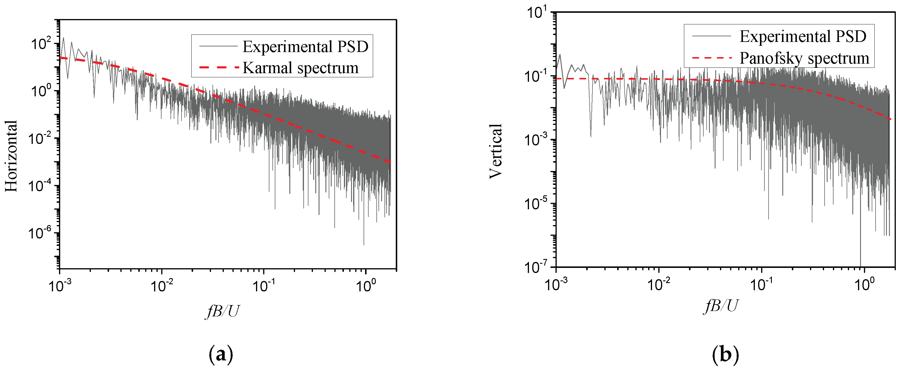
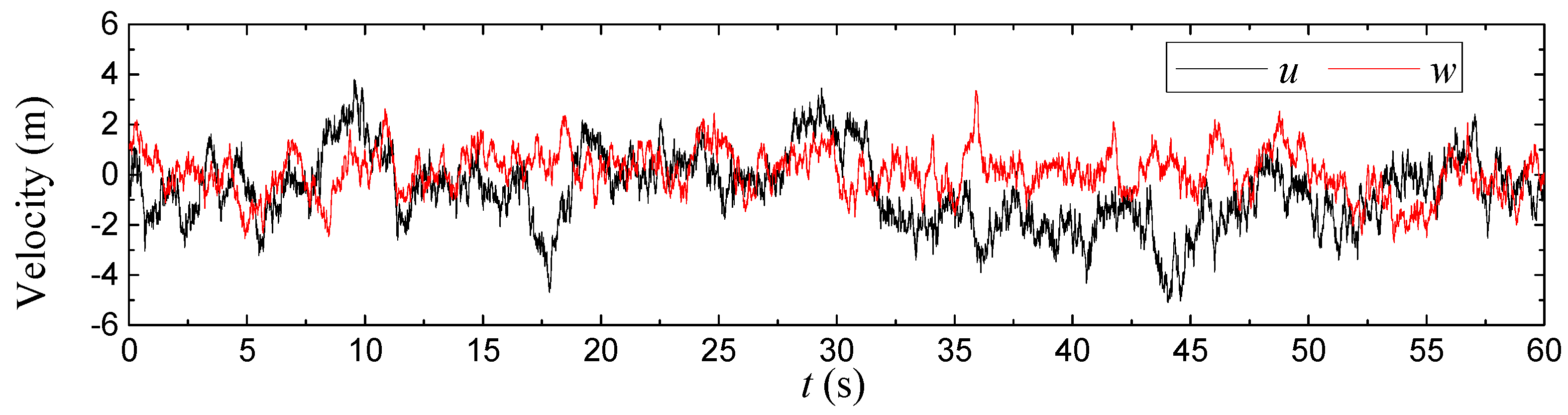
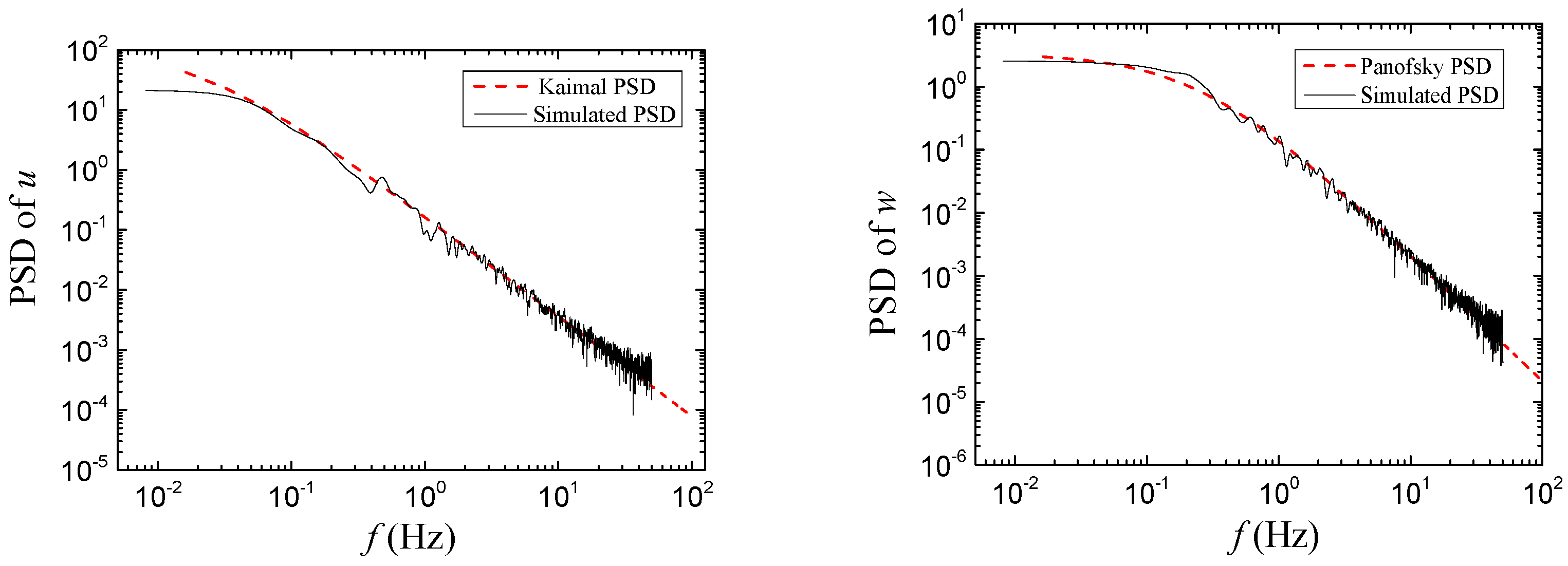
3.3. Turbulent Wind Flow Characteristics in the Wind Tunnel

The DDTG may be subjected to turbulent winds in different surrounding terrain conditions. The turbulent features appear to have a direct influence on the buffeting force on the bridge girder. Therefore, the turbulence effect on the bridge girder should be taken into account.

Usually, the turbulent flow in the wind tunnel tests was generated by spires, cubes, or a combination of them. In Bj-1, the segment model should be attached to the wind tunnel sidewalls at their mid-height (see Figure 2), and the wind field produced by the cubes had little effect on the aerodynamic force on the segment model due to their location and distance to the wind test region. Therefore, the turbulent flows in this test were only produced by four spires (1.5 m in height; see Figure 4).

The characteristics of the flows simulated in the wind tunnel were measured using a Cobra Probe (Turbulent Flow Instrumentation, Victoria, Australia) in front of the test model, at the same height as the segment model, which could resolve three components of the mean and fluctuating velocities and had a sampling frequency of up to 2,000 Hz. In this test, the sampling frequency of the probe was set to 1,024 Hz, and the sampling time was 180 s. To examine the uniformity of the turbulent flow field, the wind data were repeatedly measured at the front position of the test model. In the wind tunnel, the turbulent flow behind the spires has a horizontally isotropic character [26], while the longitudinal and vertical wind components can be described by the Kaimal spectrum (Equation (8)) [27] and Panofsky spectrum (Equation (9)) [28], respectively. Figure 5 shows a comparison between the longitudinal and vertical power spectral densities (PSDs) measured in turbulent flow fields and the target PSDs. The two curves in Figure 5a,b are mainly in good agreement. Therefore, the frequency range of the wind simulated in the wind tunnel can meet the requirements of the wind tunnel test.

$$S_u(n)={\mu }_{\ast }^2\frac{200f}{n{(1+50f)}^{5/3}}\left(\mathrm{Kaimal}\mathrm{spectrum}\right)$$

(8)

$$S_w(n)={\mu }_{\ast }^2\frac{6f}{n{(1+4f)}^{1/2}}\left(\mathrm{Panofsky}\mathrm{spectrum}\right)$$

(9)

where f = nz/U, n is the wind frequency; ${\mu }_{\ast }^{}$ is the friction velocity; and u and w indicate the longitudinal direction and vertical direction, respectively.

4. Test Results

4.1. Aerodynamic Wind Force Coefficients and Derivatives

The wind force can be decomposed into three components, the drag force, lift force and pitch moment, along the wind and body axes, as shown in Figure 6. At the initial wind attack angle α₀, the girder experiences an additional wind attack angle α₁ produced by the wind load, and the sum of α₀ and α₁ is the effective wind attack angle α. Because the segment model is attached to the load balance by a pair of rigid connectors and the model must have sufficient stiffness in the wind tunnel test, the additional wind attack angle α₁ is always so small that it can be ignored, i.e., α = α₀. The instantaneous aerodynamic wind force per unit span can be written as a function of the effective wind attack angle along the wind axes:

$$\mathrm{Drag}\mathrm{force}\mathrm{coefficient}:C_{\mathrm{D}}(\alpha ,t)=\frac{F_{\mathrm{D}}(t)}{0.5\rho U^{2}H}$$

(10)

$$\mathrm{Lift}\mathrm{force}\mathrm{coefficient}:C_L(\alpha ,t)=\frac{F_L(t)}{0.5\rho U^{2}B}$$

(11)

$$\mathrm{Pitch}\mathrm{moment}\mathrm{coefficient}:C_M(\alpha ,t)=\frac{F_M(t)}{0.5\rho U^2{B}^2}$$

(12)

where α is the effective wind attack angle and ρ is the air density. The positive direction of the wind force is shown in Figure 6, where the pitch moment is determined according to the right hand rule. The test results of the average aerodynamic force coefficients for the service and construction stages at wind attack angles of −10°~+10° are shown in Figure 7, and these wind tunnel tests were performed by the authors before the tests in this paper [29]. Usually, the aerodynamic force coefficients are fit by a polynomial, such as $y={\displaystyle \sum _{i=1}^N{a}_i{x}^{N-i}},N=1,2,3,\dots$, where N = 7 in this paper, and the fitting curves of the aerodynamic force coefficients are also shown in Figure 7.

Table 2. Aerodynamic force coefficients and derivatives for the service stage.

α (°)	${\mathit{C}}_{\mathit{D}}$	${\mathit{C}}_{\mathit{D}}^{\prime }$	${\mathit{C}}_{\mathit{L}}$	${\mathit{C}}_{\mathit{L}}^{\prime }$	${\mathit{C}}_{\mathit{M}}$	${\mathit{C}}_{\mathit{M}}^{\prime }$
0°	0.8362	−0.0139	−0.0848	0.1023	−0.0028	0.0027
3°	0.8659	0.0283	0.3035	0.1089	0.0123	0.0063
5°	0.9368	0.0424	0.4355	0.0680	0.0268	0.0102

and

Table 3. Aerodynamic force coefficients and derivatives for the construction stage.

α (°)	${\mathit{C}}_{\mathit{D}}$	${\mathit{C}}_{\mathit{D}}^{\prime }$	${\mathit{C}}_{\mathit{L}}$	${\mathit{C}}_{\mathit{L}}^{\prime }$	${\mathit{C}}_{\mathit{M}}$	${\mathit{C}}_{\mathit{M}}^{\prime }$
0°	0.7286	−0.0017	−0.1831	0.1793	0.0070	0.0043
3°	0.7864	0.0368	0.4713	0.1755	0.0196	0.0087
5°	0.8751	0.0498	0.6509	0.0892	0.0471	0.0126

show the aerodynamic force coefficients and derivatives for the service and construction stages at wind attack angles of 0°, 3° and 5°.

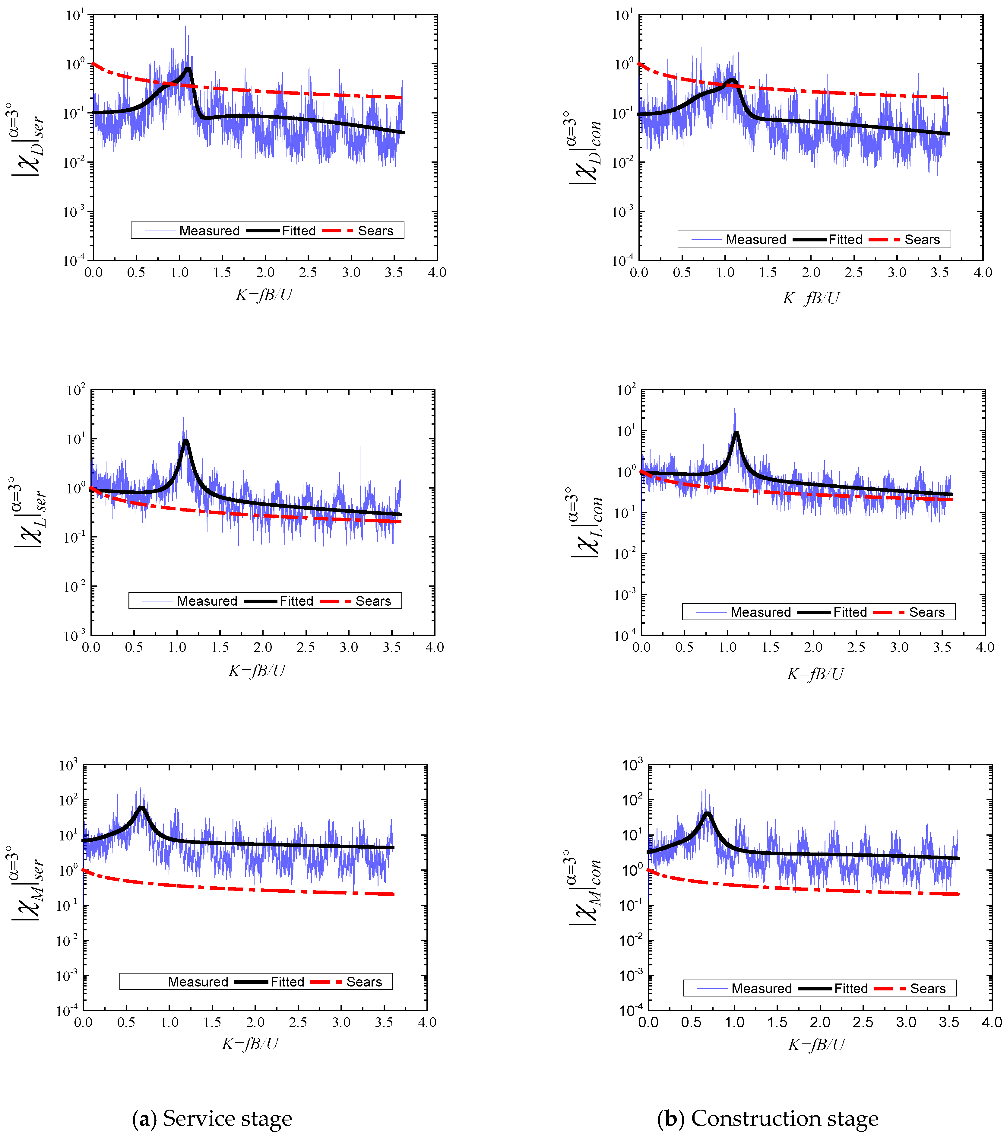
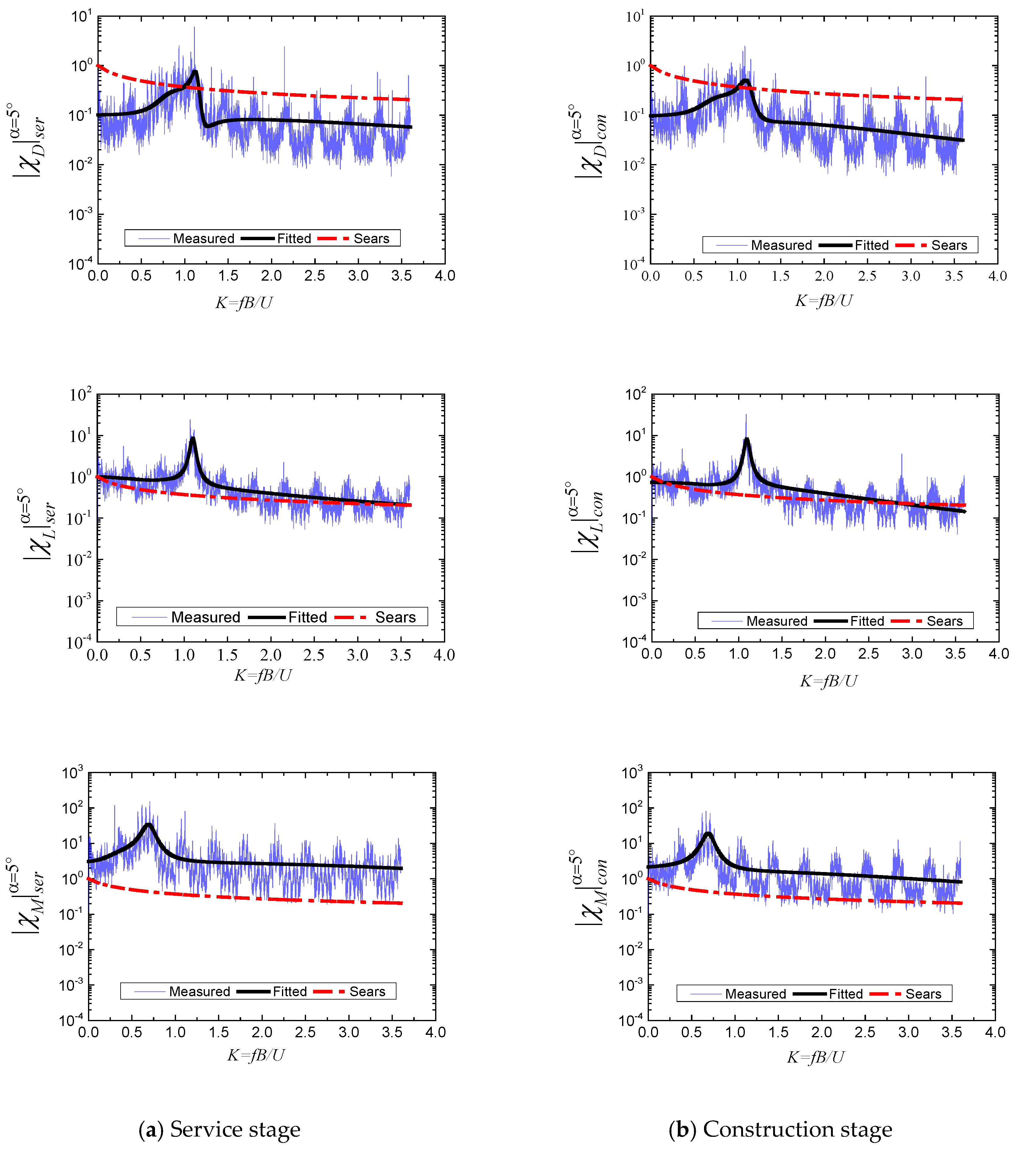
4.2. AAFs Identified by a Nonlinear Expression

Figure 8, Figure 9 and Figure 10 display the identified equivalent AAFs of the DDTG for the service and construction stages under α = 0°, α = 3° and α = 5°, respectively. According to some previous studies [18,26], the AAFs can always be fitted by nonlinear expressions, such as the first item in Equation (13). When the test system is installed completely, the system has natural frequencies of vibration in all three measured directions, which have a strong influence on the test accuracy of the force measured method. Limited by the model materials, the manufacturing technique and the connection of each component in the test system, the model resonance cannot be avoided. If only the traditional expression (the first item in Equation (13)) is used to fit AAFs, a serious distortion will occur near the natural frequencies. In this paper, a peak item is introduced to improve the fitting accuracy. Through many trials, the measured AAFs are effectively fitted using the following target nonlinear function:

$${\left|{\chi }_i(K)\right|}_{eq}=\frac{\alpha }{\tau +\beta K^r}+\frac{c_1{K}^2+c_2}{{(K-c_3)}^4+c_4{K}^2+c_5}$$

(13)

where i = D, L, M; K = fB/U is the reduced frequency; α, τ, β, γ, c₁, c₂, c₃, c₄, and c₅ are the nine parameters to be fitted; and the second item of Equation (13) on the right-hand side is used to fit the peak of the AAF in the low frequency range. Normally, for a long-span road-rail cable-stayed bridge, the wind-induced sensitive modes usually appear in the first 50 natural modes, and the reduced frequency is usually below 3.0 [30]. Thus, the reduced frequency range was chosen as 0~3.6 in this paper. When the undetermined parameters in Equation (13) were fitted, an undesired peak appeared due to model resonance. The actual AAFs used in the buffeting response analysis of the long-span bridge can be modified by eliminating the fractions in the second item of Equation (13). The identified parameters in the first item of Equation (13) are shown in

Table 4. Main parameters identified in fitting AAFs by Equation (13) at different stages.

Item	Ang.	Service Stage				Construction Stage
		α	τ	β	γ	α	τ	β	γ
$\left|{\chi }_D\right|$	0	0.1176	1.305	0.0155	3.629	0.1191	1.816	0.09806	1.699
	3	0.2966	2.985	0.0271	3.975	0.5859	6.499	0.3943	2.442
	5	5.525	55.43	2.472	2.170	0.2502	2.637	0.2139	2.509
$\left|{\chi }_L\right|$	0	0.7604	0.2978	0.3601	1.034	0.9118	0.5752	0.2288	1.779
	3	0.2108	0.2463	0.0950	1.290	0.4404	0.4932	0.1545	1.544
	5	1.961	1.970	1.054	1.533	0.5388	0.7341	0.1107	2.577
$\left|{\chi }_M\right|$	0	6.052	0.3494	0.0013	3.706	7.333	0.6799	0.0691	1.644
	3	2.432	0.3752	0.0261	1.518	2.052	0.7196	0.0015	3.937
	5	1.960	0.6928	0.0062	3.050	1.241	0.6413	0.0117	2.577

.

In each figure, the modulus of the Sears function derived for the lift force of an aerofoil or a flat plate is also plotted. The Sears function significantly deviates from most measured AAFs of the DDTG in the service and construction stages. The major reason is probably that the Sears function is appropriate only for the lift force AAF of an aerofoil, an ideal flat plate or a flat streamlined box girder section, and the aerofoil section greatly differs from the truss bridge section in this study. In the turbulence, the vertical and oblique web members (see Figure 1) changed the inner flow field between roadway and railway decks, and led the changes of the energy transfer from turbulence to buffeting forces.

As the DDTG has a high ventilation rate (58%), there is less wind energy transfer to the structural wind load than the ideal flat with the same height of the DDTG. Therefore, the value of identified $\left|{\chi }_D\right|$ is always below the Sears function. Comparing the measured $\left|{\chi }_L\right|$ with the Sears function, similar tendencies are observed between these two AAFs because the double decks of the DDTG have wide flat characteristics and little aerodynamic impact between them. It is generally recognized that the $\left|{\chi }_L\right|$ and $\left|{\chi }_M\right|$ have the approximate frequency of peak value in box girder or ideal flat [18]. However, unlike an ideal flat, the different peak frequencies of the DDTG between the lift and torsional equivalent admittances in each stage is significant. The reason is probably that the influence degrees and frequency ranges of the vertical and torsional resonances of the measured system for the lift and pitch moment are different. Another possible reason is that in the upper and lower decks, the vertical oblique web members have a choke area, and the pitch moment is produced not only by the unbalanced lift force on the double decks but also by the drag force away from the torsion centre produced by these web members.

Figure 11 shows the fitted AAFs under different wind attack angles without the peak item. For the ${\left|{\chi }_D\right|}_{ser}$ of the service stage, the sensitive frequency region of wind attack angles is the region of K > 2.0. In the construction stage, the ${\left|{\chi }_D\right|}_{con}$ becomes more sensitive with changes in the wind attack angles: in the region of K < 3.0, the ${\left|{\chi }_D\right|}_{con}$ gradually increases with the wind attack angle from 0° to 5°, but shows an opposite phenomenon in the region of K ≥ 3.0. Compared to the ${\left|{\chi }_L\right|}_{ser}$ and ${\left|{\chi }_L\right|}_{con}$, these two AAFs have the largest value when α = 0°, especially in the region of K < 3.0, which indicates that the lift force has more energy that makes it easier to cause the vertical vibration of the DDTG. Similarly, the ${\left|{\chi }_M\right|}_{ser}$ and ${\left|{\chi }_M\right|}_{con}$ make it easier to cause the torsional vibration of the DDTG when α = 0°.

5. AAF Numerical Application

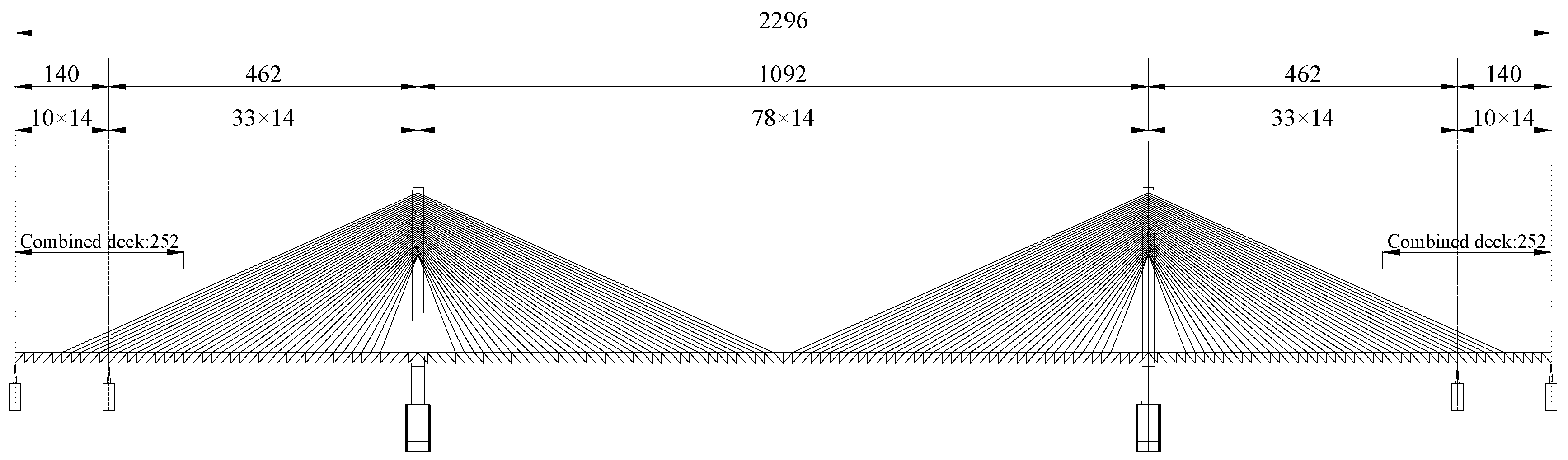
5.1. Description of the Case Bridge

The case bridge over the Yangtze River is a cable-stayed roadway-railway bridge with a central span of 1092 m and a total length of 2296 m. For the navigation and structural requirements, an auxiliary pier is set at each side span 140 m from the bridge end. The span arrangements of the case bridge are 140 + 462 + 462 + 1092 + 462 + 140 m (Figure 12). The girder section is similar to that shown in Figure 1a. Two 252 m concrete–steel combined segments, with a 0.45 m thickness of the concrete highway deck, are applied in the side spans to increase the stiffness of the side spans and balance the negative reaction of the auxiliary piers. The average elevation of the girder is approximately 80 m, and the design wind speed at the girder location is 49.8 m/s. The vertical wind profiles at the bridge site satisfy an exponential law, and the surface roughness coefficient is 0.12.

5.2. Numerically Equivalent Model of the DDTG

A 3D finite element model (3D model for short) of the case bridge was established with the commercial software ANSYS, as shown in Figure 13a. It was developed using APDL code, and all structural components, connections and boundary conditions of the bridge were properly simulated. The beam188 is a kind of bar element, which allows the users to apply a real section of the truss component. The shell181 element is suitable for the shell structure with medium thickness. Therefore, in the 3D model, the truss bars are modelled by 3D beam188 elements with real sections, and the bridge decks are modelled by shell181 elements. For the combined roadway and steel decks, the different girder types are shown in Figure 14a,b. The main simplification considered herein to reduce the computational effort of the buffeting analyses, especially for the partial members of the DDTG, is to put forward an equivalent “fish-bone” model to replace the 3D model while retaining the global mechanical behaviour of the DDTG. The fish-bone model was also established in ANSYS, as shown in Figure 13b. The fish-bone model was adopted for the nonlinear transient analyses. The beam4 element has only mechanical characteristics of the section, which is appropriate for simulating the virtual girder of the fish-bone model. In the model, the girder is modelled by beam4 elements with equivalent static and dynamic mechanical characteristics, as shown in

Table 5. Static and dynamic parameters of the equivalent fish-bone model of the girder.

Parameters	Value
Weight per metre of composite girder	87,029 kg/m
Weight per metre of steel girder	48,873 kg/m
Additional highway concrete deck load	9102.04 kg/m
Additional highway steel deck load	5469.39 kg/m
Additional railway load	28,440 kg/m
Material damping ratio	0.005

and

Table 6. Inertia moment of the fish-bone model girder (m⁴).

Section Type	Ixx	Iyy	Izz
Composite girder	687.8	168.6	679.3
Steel girder	273.3	108.6	502.3

, connected with cables by rigid elements. The cables are modelled by the tension-only element, link10 elements, to account for the geometric nonlinearity according to the sag. The towers are modelled by beam4 elements, along with their mechanical properties, in all models.

To ensure the accuracy of the fish-bone model’s dynamic properties, the natural frequencies of the 3D and fish-bone models were carefully checked and compared. A modal analysis with the Block Lanczos method was applied to compare the primary natural modes and frequencies of the 3D model and fish-bone model, as listed in

Table 7. Comparison of the primary natural frequencies and mode descriptions of the 3D and fish-bone models.

Mode Description	Frequency (Hz)
	3D Model	Fish-Bone	Err. (%)
1st sym lateral bending movement	0.1013	0.1032	1.88%
1st sym vertical bending movement	0.1920	0.1990	3.65%
1st asym vertical bending movement	0.2713	0.2731	0.66%
1st asym lateral bending movement	0.2810	0.2928	4.2%
2nd sym vertical bending movement	0.4340	0.4630	6.68%
2nd asym vertical bending movement	0.4405	0.4479	1.68%
1st sym torsional and weak lateral bending movement	0.4590	0.4726	2.96%
2nd asym lateral bending movement	0.4777	0.5072	6.18%

*‘sym’ for symmetric; ‘asym’ for antisymmetric; ‘Err’ for error of the fish-bone model relative to the 3D model.

. According to the frequency result comparisons, the fish-bone model includes most vibration modes and mechanical properties of the 3D model, which proves that the equivalent fish-bone model can replace the 3D model in buffeting analysis. Due to the paper limitations, only the 1st symmetric lateral, vertical and torsional and antisymmetric vertical mode shape comparisons are shown in Figure 15, which indicates that the two models have good consistency in the dominant mode shape of the buffeting analysis. The natural frequencies of the lateral and vertical deflections are always low, which illustrates that the stiffness of the girder in both directions is small and that deformation may occur more easily in these directions than in other directions in the buffeting analysis. The results of the modal analysis indicate that the response of the case bridge under a turbulent wind load can be assumed to be dominated by lateral and vertical deflections.

5.3. Stochastic Modelling of the Wind Field at the Bridge Site

The turbulent wind field at a bridge site is generally determined by the orography and the environment. In this paper, a numerical wind field is used to derive the wind forces on the case bridge. The numerical turbulent wind field is described in stochastic theory by Solari [31], while its realizations are obtained on the basis of the wind velocity generation procedure of Di [32]. In a numerical wind field, the wind is simulated as a spatially correlated stochastic process acting in the horizontal and vertical directions. The simulated wind U(t) is assumed to be an n-dimensional stochastic vector process that can be decomposed into a summation of n n-dimensional fully coherent normal vectors Y_j(t) independent of each other, as shown in Equation (14) and Equation (15). For all the symbols and the derivation process, refer to the relevant literature [31,32,33].

$$U(t)={\displaystyle \sum _{i=1}^n{Y}_j(t)}$$

(14)

$$Y_j(t)=2{\displaystyle \sum _{k=1}^N{H}_j(f_k)\sqrt{{\mathsf{\Lambda }}_j(f_k)\Delta f_k}\left[\cos (2\pi f_{k}t)-I_k^j\sin (2\pi f_{k}t)\right]}$$

(15)

In this paper, a 5-point wind field with a 1 m horizontal interval was generated to verify the wind history generated using the aforementioned method. The Kaimal spectrum was applied for the PSD of the horizontal turbulent wind component u (Equation (8)), and the Panofsky spectrum was applied for the PSD of the vertical turbulent wind component w (Equation (9)). Figure 16 shows the 60 s wind history at one point in the simulated wind field, and Figure 17 shows the comparison between the simulated and target PSDs. The simulated turbulent wind PSDs agree well with the target design value.

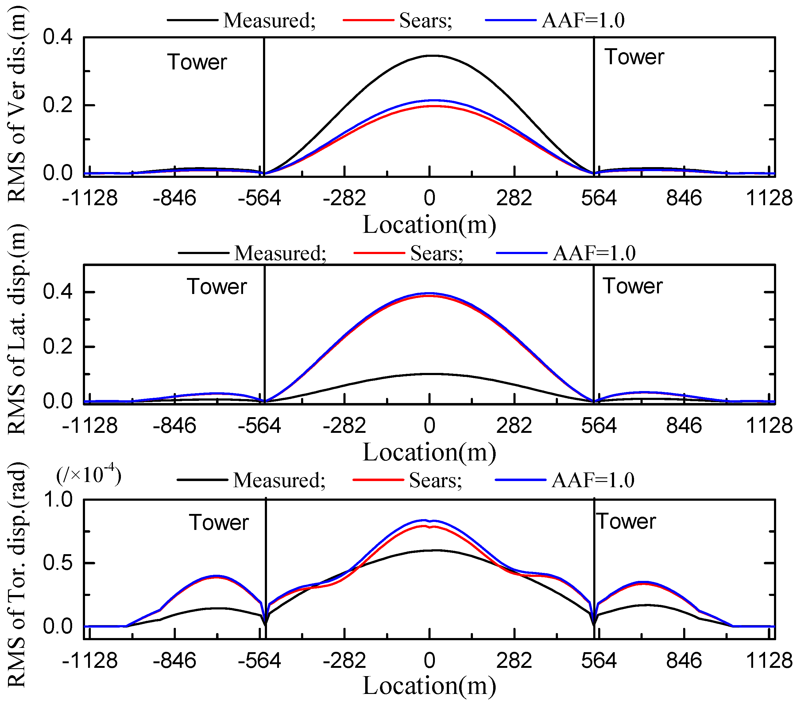
5.4. Buffeting Response Obtained Using Multiple AAF Types

The buffeting responses of the case cable-stayed bridge were calculated using a nonlinear transient FE approach. Three types of AAFs were taken into consideration in the calculation, i.e., AAF = 1.0, the Sears function and the identified AAFs previously mentioned. AAF = 1.0 corresponds to completely neglecting the correction of the unsteady effect on the quasi-steady buffeting forces in the AAFs. In the calculation, the wind speed at the girder is set at the design speed of 49.8 m/s, and the oncoming wind is lateral and normal to the bridge span. The calculated root-mean square (RMS) values of the lateral, vertical and torsional displacements under the service and construction stages are plotted in Figure 18 and Figure 19, respectively. The PSDs of the buffeting displacements at the mid-span centre point are plotted in Figure 20.

According to Figure 18 and Figure 19, the calculated vertical, lateral and torsional buffeting responses based on the identified AAFs deviate from those based on the Sears function and 1.0 AAFs. The RMS reflects the vibration amplitude of the DDTG in turbulence. The RMS of the Sears function is very close to the RMS obtained when neglecting the correction of the unsteady force. However, the RMS by these two AAF types always have disparity with identified AAFs. Furthermore, because the Sears function is greater than the identified AAF in terms of $\left|{\chi }_D\right|$ for both the service and construction stages mentioned above, the lateral response calculated based on the identified AAFs is much lower in each stage. Similarly, the Sears function is less than the identified AAF in terms of $\left|{\chi }_L\right|$, so the vertical RMS of the identified AAFs is 1.75 times larger than that of the Sears function in the service stage and 2.0 times in the construction stage (see

Table 8. RMS maximum value of mid-span in the service and construction stages.

Direction	Service Stage			Construction Stage
	Measured	Sears	1.0	Measured	Sears	1.0
Vertical disp.(m)	0.346	0.198	0.215	0.312	0.156	0.171
Lateral disp.(m)	0.101	0.386	0.396	0.073	0.271	0.280
Torsion disp. (rad/×10−5)	6.008	7.925	8.391	10.12	10.62	10.90

). Hence, if the wind resistant design for the DDTG using the Sears function or AAF = 1.0, an unreasonable and unsafe stiffness design for the girder is produced with severe low vertical stiffness and an excessive safety factor for lateral stiffness. Due to the high torsional rigidity of the DDTG, the torsion RMS is relatively small, and the difference among each AAF of $\left|{\chi }_M\right|$ is almost negligible.

For long-span bridges, like the case one, the vibration of the girder is most controlled by the modal in the low frequency region (f ≤ 2.0Hz for the case bridge). In Figure 20, some obvious differences are observed between the buffeting response PSDs obtained using the three kinds of AAFs. When ignoring the correction of the unsteady effect on the quasi-steady buffeting forces using AAF = 1.0, the buffeting response PSDs of the DDTG are the largest for all of the structural stages. It follows that the energy transfer from the wind spectrum to the buffeting force spectrum is incomplete, and the energy loss cannot be ignored. Usually, the Sears function is set as the AAF for a single deck section and derived from the wind lift pressure/force on a single deck. Although the decks of the DDTG are wide and flat, the wind flow in the space between the double decks also has the wind pressure/force on the roadway and railway decks. Combined with Table 7, lateral vibration easily occurs in the long-span cable-stayed bridge with the DDTG. As the identified AAF ${\left|{\chi }_D\right|}_{ser}$ and ${\left|{\chi }_D\right|}_{con}$ are rather lower than the Sears function for both service and construction stages, the lateral response PSDs, based on identified AAF, are quite small in the low frequency region (f ≤ 2.0 Hz or reduced frequency K ≤ 1.4) Comparing the response PSDs between the service and construction stages, the deck appendants, such as the road handrail and railway slag wall, only affect the torsional PSD because the deck appendants change the turbulence flow over the road deck and the truss internal space.

6. Conclusions

This paper describes aerodynamic admittance investigations conducted for the DDTG used in long-span rail-road cable-stayed bridges. A series of wind tunnel tests were performed based on force measurements to identify the AAFs. A long-span rail-road cable-stayed bridge was used to compare the identified AAFs with two other AAFs (AAF = 1.0 and the Sears function) in terms of the buffeting response. The following conclusions were obtained from this study:

• The AAFs of the DDTG were successfully obtained in the target turbulent wind field through wind tunnel tests based on the force measurement method. Typical service/construction stages and multiple wind attack angles (0°, 3° and 5°) were considered in the wind tunnel tests to identify the AAFs of the DDTG.
• In order to reduce fitting distortion caused by the resonance of the test system in the force measurement method, a modified nonlinear express was put forward to fit the AAFs of the DDTG in this paper. In the nonlinear expression, an additional item was introduced to fit the peak caused by resonance of the test system, and the traditional item was applied to fit the other unaffected experimental value. The combination of these two items can more efficiently match the experimental results of AAFs.
• According to the comparison between the identified AAFs of the DDTG and Sears functions, the Sears function is not applicable to the DDTG in both service and construction stages. With the α changing from 0° to 5°, the ${\left|{\chi }_D\right|}_{con}$ has a greater sensibility to the wind attack angle. When α = 0°, the vertical and torsion vibration occur more easily in the DDTG because the ${\left|{\chi }_L\right|}_{}$ and $\left|{\chi }_M\right|$ both have larger values than the other wind attack angles.
• A “fish-bone” model with an equal mechanical property to the DDTG is put forward in this paper to compensate for the computational insufficiency of the 3D finite element model in the transient analysis. Through modal analysis, these two models almost have a similar mode shape and frequency, which confirmed the equivalence of these two models in dynamic analysis.
• According to the buffeting response comparison for three kinds of AAFs (AAF = 1.0, the Sears function and the identified AAFs), the Sears function or AAF = 1.0 leads to an inaccurate response estimation for the DDTG. The Sears function and AAF = 1.0 underestimate the vertical vibration amplitude and overestimate the lateral vibration amplitude in DDTG wind-resistant design.

References

1. He, X.; Wu, T.; Zou, Y.; Chen, Y.F.; Guo, H.; Yu, Z. Recent developments of high-speed railway bridges in China. Struct. Infrastruct. Eng. 2017, 13, 1584–1595. [Google Scholar] [CrossRef]
2. Sears, W.R. Some aspects of non-stationary airfoil theory and its practical application. J. Aeronaut. Sci. 1941, 8, 104–108. [Google Scholar] [CrossRef]
3. Liepmann, H.W. On the application of statistical concepts to the buffeting problem. Aeronaut. Sci. 1952, 1, 793–800. [Google Scholar] [CrossRef]
4. Liepmann, H.W. Extension of the Statistical Approach to Buffeting and Gust Response of Wings of Finite Span. J. Aeronaut. Sci. 1955, 22, 197–200. [Google Scholar] [CrossRef]
5. Graham, J.M.R. Lifting Surface Theory for the Problem of an Arbitrarily Yawed Sinusoidal Gust Incident on a Thin Aerofoil in Incompressible Flow. Aeronaut. Q. 1970, 21, 182–198. [Google Scholar]
6. Graham, J.M.R. A Lifting-Surface Theory for the Rectangular Wing in Non-Stationary Flow. Aeronaut. Q. 1971, 22, 83–100. [Google Scholar]
7. Filotas, L.T. Theory of Airfoil Response in a Gusty Atmosphere. Part II. Response to Discrete Gusts of Continuous Turbulence; University of Toronto: Toronto, ON, Canada, 1969. [Google Scholar]
8. Filotas, L.T. Theory of Airfoil Response in a Gusty Atmosphere. Part, I. Aerodynamic Transfer Function; University of Toronto: Toronto, ON, Canada, 1969. [Google Scholar]
9. Mugridge, B.D. Gust Loading on a Thin Aerofoil. Aeronaut. Q. 1971, 22, 301–310. [Google Scholar]
10. Li, S.; Li, M.; Liao, H. The lift on an aerofoil in grid-generated turbulence. J. Fluid Mech. 2015, 771, 16–35. [Google Scholar] [CrossRef]
11. Massaro, M.; Graham, J.M.R. The effect of three-dimensionality on the aerodynamic admittance of thin sections in free stream turbulence. J. Fluid Struct. 2015, 57, 81–90. [Google Scholar] [CrossRef]
12. Jancauskas, E.D.; Melbourne, W.H. The aerodynamic admittance of two-dimensional rectangular section cylinders in smooth flow. J. Wind Eng. Ind. Aerodyn. 1986, 23, 395–408. [Google Scholar] [CrossRef]
13. Scanlan, R.H. The action of flexible bridges under wind, II: Buffeting theory. J. Sound Vib. 1978, 60, 201–211. [Google Scholar] [CrossRef]
14. Costa, C.; Borri, C.; Flamand, O.; Grillaud, G. Time-domain buffeting simulations for wind–bridge interaction. J. Wind Eng. Ind. Aerodyn. 2007, 95, 991–1006. [Google Scholar] [CrossRef]
15. Hatanaka, A.; Tanaka, H. Aerodynamic admittance functions of rectangular cylinders. J. Wind Eng. Ind. Aerodyn. 2008, 96, 945–953. [Google Scholar] [CrossRef]
16. Diana, G.; Resta, F.; Zasso, A.; Belloli, M.; Rocchi, D. Forced motion and free motion aeroelastic tests on a new concept dynamometric section model of the Messina suspension bridge. J. Wind Eng. Ind. Aerodyn. 2004, 92, 441–462. [Google Scholar] [CrossRef]
17. Larose, G.L.; Mann, J. Gust loading on streamlined bridge decks. J. Fluid Struct. 1998, 12, 511–536. [Google Scholar] [CrossRef]
18. Zhu, L.; Zhou, Q.; Ding, Q.; Xu, Z. Identification and application of six-component aerodynamic admittance functions of a closed-box bridge deck. J. Wind Eng. Ind. Aerodyn. 2018, 172, 268–279. [Google Scholar] [CrossRef]
19. Larose, G.L. Experimental determination of the aerodynamic admittance of a bridge deck segment. J. Fluid Struct. 1999, 13, 1029–1040. [Google Scholar] [CrossRef]
20. Sato, H.K.M.M. Evaluation of aerodynamic admittance for the stiffening girder of the Akashi Kaikyo Bridge. In Proceedings of the 13th Japan National Symposium on Wind Engineering, Tokyo, Japan, November 1994; pp. 131–136. [Google Scholar]
21. Xu, Y.L.; Sun, D.K.; Ko, J.M.; Lin, J.H. Buffeting analysis of long span bridges: A new algorithm. Comput. Struct. 1998, 68, 303–313. [Google Scholar] [CrossRef]
22. Scanlan, R.H.; Jones, N.P. A form of aerodynamic admittance for use in bridge aeroelastic analysis. J. Fluid Struct. 1999, 13, 1017–1027. [Google Scholar] [CrossRef]
23. Chen, X.; Matsumoto, M.; Kareem, A. Time domain flutter and buffeting response analysis of bridges. J. Eng. Mech. 2000, 126, 7–16. [Google Scholar] [CrossRef]
24. Davenport, A.G. Buffeting of suspension bridge by storm winds. J. Struct. Div. 1962, 88, 233–270. [Google Scholar]
25. Gu, M.; Qin, X. Direct identification of flutter derivatives and aerodynamic admittances of bridge decks. Eng. Struct. 2004, 26, 2161–2172. [Google Scholar] [CrossRef]
26. Li, S.; Li, M.; Larose, G.L. Aerodynamic admittance of streamlined bridge decks. J. Fluid Struct. 2018, 78, 1–23. [Google Scholar] [CrossRef]
27. Kaimal, J.C.; Wyngaard, J.C.; Izumi, Y.; Coté, O.R. Spectral characteristics of surface-layer turbulence. Q. J. R. Meteorol. Soc. 1972, 98, 563–589. [Google Scholar] [CrossRef] [Green Version]
28. Panofsky, H.A.; McCormick, R.A. The spectrum of vertical velocity near the surface. Q. J. R. Meteorol. Soc. 1960, 86, 495–503. [Google Scholar] [CrossRef]
29. Liu, H.S.; Lei, J.Q. Identification of three-component coefficients of double deck truss girder for long-span bridge. J. Zhejiang Univ. (Eng. Sci.) 2019, 53, 1–9. [Google Scholar]
30. Yu, T.; Shixiong, Z.; Longqi, Z. Numerical method for identifying the aerodynamic admittance of bridge deck. Acta Aerodyn. Sin. 2015, 33, 706–713. [Google Scholar]
31. Solari, G.; Piccardo, G. Probabilistic 3-D turbulence modeling for gust buffeting of structures. Probabilist Eng. Mech. 2001, 16, 73–86. [Google Scholar] [CrossRef]
32. Di Paola, M.; Gullo, I. Digital generation of multivariate wind field processes. Probabilist Eng. Mech. 2001, 16, 1–10. [Google Scholar] [CrossRef]
33. Domaneschi, M.; Martinelli, L.; Po, E. Control of wind buffeting vibrations in a suspension bridge by TMD: Hybridization and robustness issues. Comput. Struct. 2015, 155, 3–17. [Google Scholar] [CrossRef]
Figure 1. Cross section of the roadway-railway truss bridge: (a) girder cross section (unit: cm) and (b) 3D bridge girder with 5 truss units (unit: m).
Applsci 09 01818 g001
Figure 2. The segment model in the wind tunnel.
Applsci 09 01818 g002
Figure 3. Cross section of the segment model for the service and construction stages: (a) for the service stage; (b) for the construction stage.
Applsci 09 01818 g003
Figure 4. Experimental setups of turbulent flows (m): (a) spires in the wind tunnel; (b) set of spires (unit: m).
Applsci 09 01818 g004
Figure 5. Comparison between experimental and target PSDs: (a) longitudinal wind fluctuations; (b) vertical wind fluctuations.
Applsci 09 01818 g005
Figure 6. Three components of the wind load along different axes.
Applsci 09 01818 g006
Figure 7. Wind force coefficients at wind attack angles of −10°~+10° (‘Exp’ for experimental value; ‘Fitted’ for fitted value).
Applsci 09 01818 g007
Figure 8. AAFs (aerodynamic admittance functions) identified for the DDTG under the service and construction stages at α = 0°.
Applsci 09 01818 g008
Figure 9. AAFs identified for the DDTG under the service and construction stages at α = 3°.
Applsci 09 01818 g009
Figure 10. AAFs identified for the DDTG under the service and construction stages at α = 5°.
Applsci 09 01818 g010
Figure 11. Fitted AAFs for the DDTG without the peak item in Equation (13).
Applsci 09 01818 g011
Figure 12. Configuration of the case bridge (unit: m).
Applsci 09 01818 g012
Figure 13. The 3D and equivalent “fish-bone models” of the case bridge.
Applsci 09 01818 g013
Figure 14. Segment model of different girder types.
Applsci 09 01818 g014
Figure 15. Mode shape comparisons of the 3D and fish-bone models: (a) Mode 1; (b) Mode 2; (c)Mode 3; (d) Mode 7.
Applsci 09 01818 g015
Figure 16. Sample of turbulent wind velocity obtained by the described procedure (U = 10 m/s).
Applsci 09 01818 g016
Figure 17. PSDs of different turbulent components in the simulated wind field.
Applsci 09 01818 g017
Figure 18. RMS of the truss girder displacements at the service stage under different AAFs.
Applsci 09 01818 g018
Figure 19. RMS of the truss girder displacements at the construction stage under different AAFs.
Applsci 09 01818 g019
Figure 20. Buffeting response PSDs at the mid-span centre point under different AAFs.
Applsci 09 01818 g020