Virtual Object Replacement Based on Real Environments: Potential Application in Augmented Reality Systems


Abstract
:1. Introduction
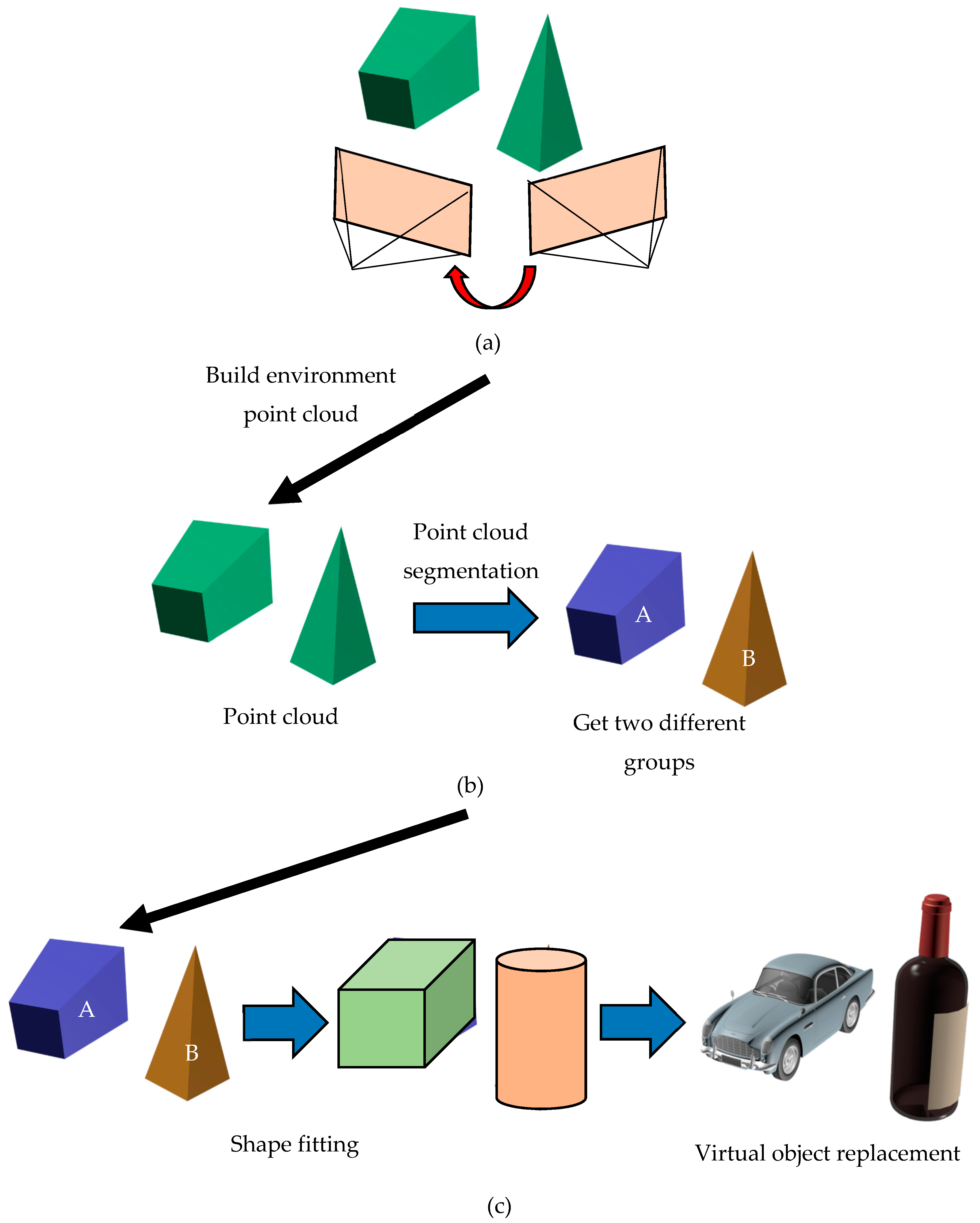
- We developed a comprehensive rendering system combining mapping, point cloud segmentation, and shape fitting.
- In point cloud segmentation, local loop closure optimization is used to reduce local errors, and global loop closure eliminates errors from the positions pertaining to the origin and destination, without affecting the segmented map.
- Prior to point cloud segmentation, supervoxel generation and plane detection are used for preprocessing methods aimed at reducing the number of segments and overall computation time.
2. Related Work
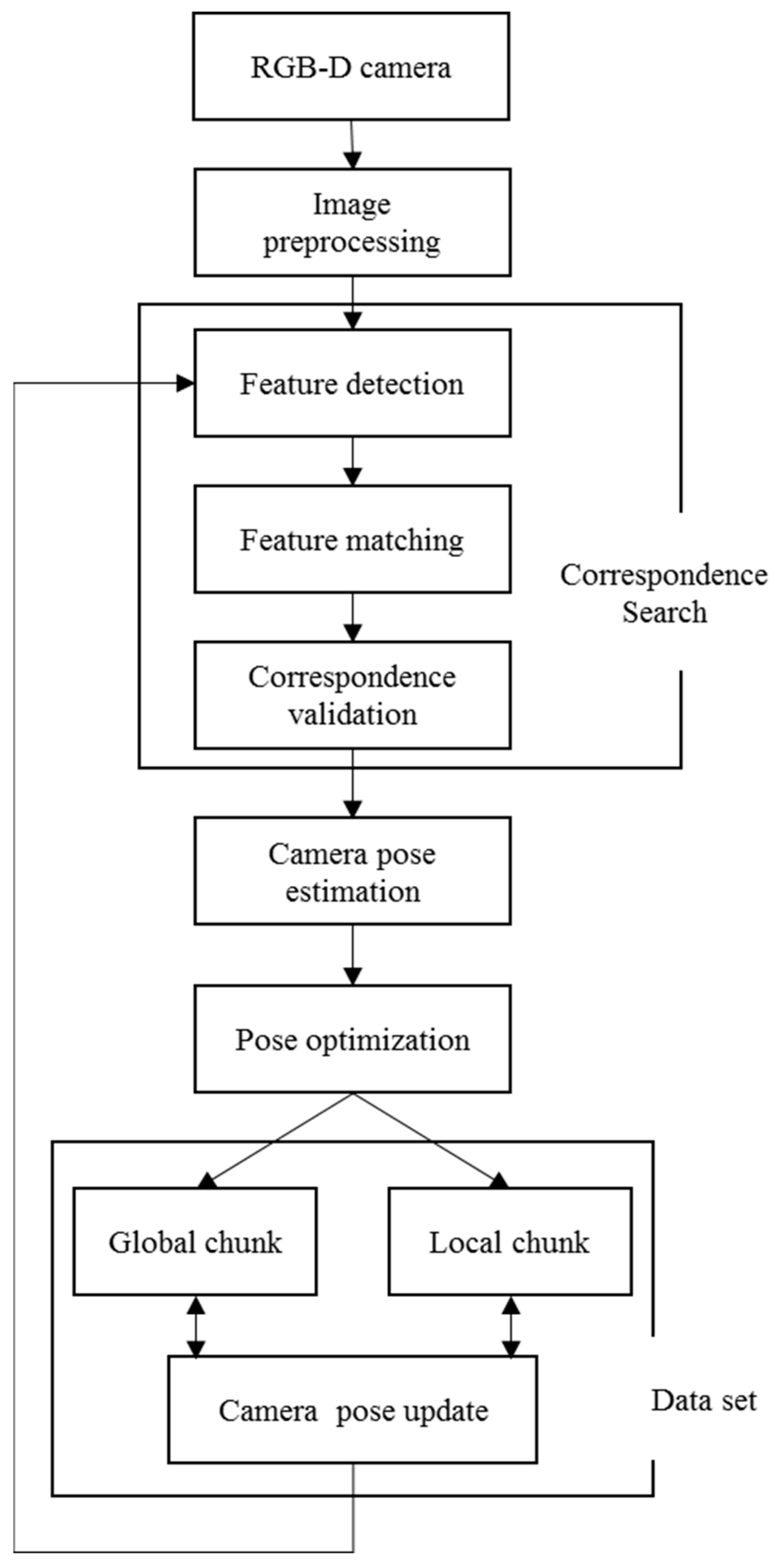
3. Mapping
3.1. Image Preprocessing
3.2. Feature Extraction and Matching
3.3. Pose Optimization
4. Point Cloud Segmentation
4.1. Supervoxel Generation
4.2. Plane Detection
4.3. Graph-Based Segmentation
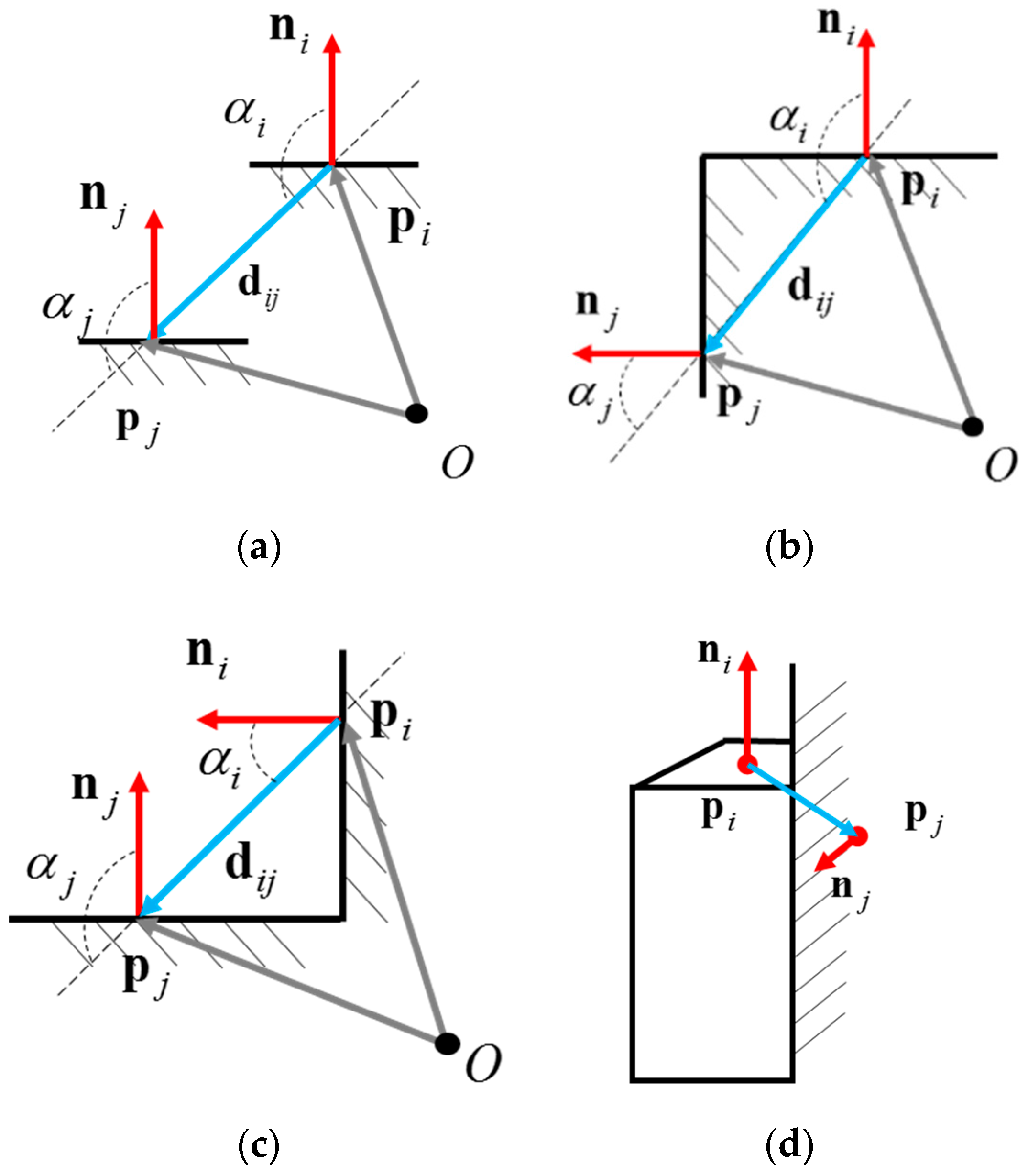
4.3.1. Graph Construction
4.3.2. Graph Construction
4.3.3. Segmentation Post-Processing
5. Shape Fitting
5.1. Inside-Outside Function
5.2. Initial Parameter Settings
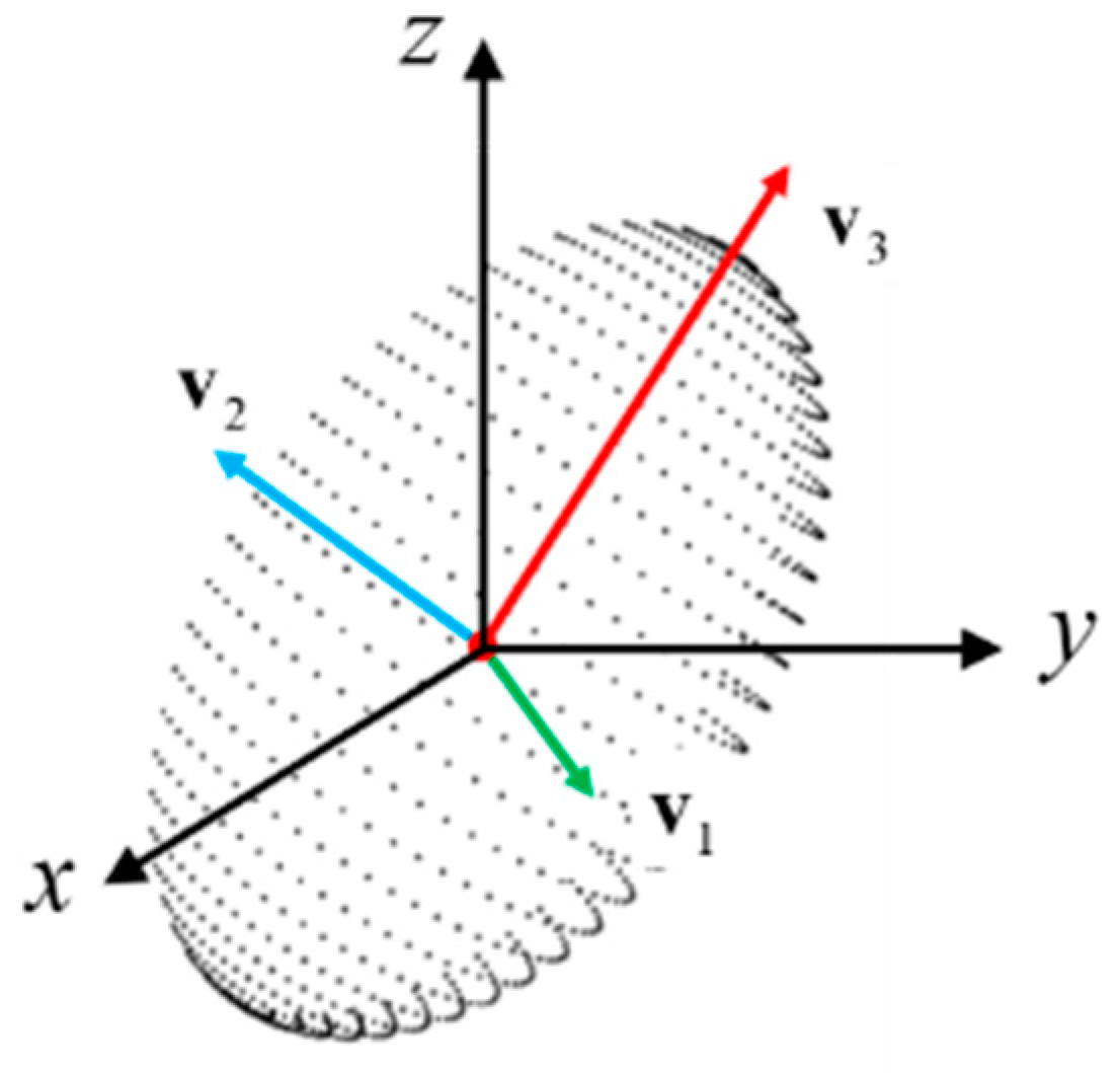
5.3. Point Group Normalization
6. Experiments and Discussion
6.1. System Description
6.2. Verification of the Proposed Rendering System
7. Conclusions
7.1. Implementation Scenario
7.2. Limitations
7.3. Future Work
Author Contributions
Funding
Conflicts of Interest
Abbreviation
| Symbol | Definition |
| a1, a2, a3 | Dimensions of the superquadric on the various axes |
| aj | Intrinsic and extrinsic camera parameters of image j |
| bi | 3D point i |
| d | Vector of two points |
| E | Reprojection error |
| E | A set of similarity values |
| e | Similarity of the edges |
| F(x,y,z) | Function to determine whether a given point is on the inside or outside of the superquadric |
| Ii, Ij | Internal difference of a component |
| K | Intrinsic parameter matrix of the camera |
| k | Number of top eigenvectors |
| l | Mean distance between the point and the center |
| ni, nj | Normal directions of two points |
| P | Points in a 3D space on the image plane |
| pi, pj | Centers of the supervoxels |
| px,py,pz | Parameters of the translation matrix |
| Q(aj,bi) | Projection point of object point bi under camera parameters aj |
| s | External product of the normal directions |
| s | Scaling rate |
| Number of points within point group S | |
| Si | A single group |
| sx,sy,sz | Scaling ratios |
| u,v | Coordinates of the image plane |
| v1,v2,v3 | Eigenvectors of the point group |
| Vi | A supervoxel point |
| vi, vj | Supervoxels |
| x,y,z | Coordinates of a point on the superquadric |
| Center of the point group | |
| Camera coordinate of points | |
| xij | Point i seen in image j |
| xj | jth piece of image sample |
| World coordinate of points | |
| αi, αj | Angles used to define the type of adjacency between points |
| δ | Threshold value used in image segmentation |
| δdepth | Threshold value used in image matching |
| ε1, ε2 | Shape of the superquadric |
| η,ω | Surface parameters of superquadric |
| θ,f,ψ | Parameters of the rotation matrix |
| θthresh | Threshold value used to determine the type of stair-like adjacency |
| τ | Maximum degree of internal similarity |
| ωij | Degree of similarity between two neighboring points |
References
- LaValle, S.M. Virtual Reality; Cambridge University Press: Cambridge, UK, 2016. [Google Scholar]
- Dieter, S.; Tobias, H. Augmented Reality: Principles and Practice; Addison-Wesley Professional: Boston, MA, USA, 2016; ISBN 0321883578. [Google Scholar]
- Yang, L.; Noelle, R.B.; Markus, M. Augmented Reality Powers a Cognitive Prosthesis for the Blind. Available online: https://doi.org/10.1101/321265 (accessed on 22 May 2018).
- Evans, G.; Miller, J.; Pena, M.I.; MacAllister, A.; Winter, E. Evaluating the Microsoft HoloLens through an augmented reality assembly application. In Proceedings of the SPIE Defense, Anaheim, CA, USA, 7 May 2017; pp. 1–16. [Google Scholar]
- Cui, N.; Kharel, P.; Gruev, V. Augmented reality with Microsoft HoloLens holograms for near infrared fluorescence based image guided surgery. In Molecular-Guided Surgery: Molecules, Devices, and Applications III; SPIE: Bellingham, WA, USA, 2017; Volume 10049. [Google Scholar] [CrossRef]
- Davison, A.J.; Reid, I.D.; Molton, N.; Stasse, O. MonoSLAM: Real-time single camera SLAM. IEEE Trans. Pattern Anal. Mach. Intell. 2007, 29, 1052–1067. [Google Scholar] [CrossRef] [PubMed]
- Klein, G.; Murray, D. Parallel tracking and mapping for small AR workspaces. In Proceedings of the Sixth IEEE and ACM International Symposium on Mixed and Augmented Reality, Nara, Japan, 1 November 2007; pp. 225–234. [Google Scholar]
- Klein, G.; Murray, D. Improving the agility of key frame-based SLAM. In Proceedings of the European Conference on Computer Vision, Marseille, France, 12–18 October 2008; pp. 802–815. [Google Scholar]
- Klein, G.; Murray, D. Parallel tracking and mapping on a camera phone. In Proceedings of the Eighth IEEE and ACM International Symposium on Mixed and Augmented Reality, Orlando, FL, USA, 19–22 October 2009; pp. 83–86. [Google Scholar]
- Mur-Artal, R.; Montiel, J.; Tardos, J. ORB-SLAM: A versatile and accurate monocular SLAM system. IEEE Trans. Robot. 2015, 31, 1147–1163. [Google Scholar] [CrossRef]
- Engel, J.; Sturm, J.; Cremers, D. Semi-Dense Visual odometry for a monocular camera. In Proceedings of the IEEE International Conference on Computer Vision, Sydney, NSW, Australia, 1–8 December 2013; pp. 1449–1456. [Google Scholar]
- Engel, J.; Schöps, T.; Cremers, D. LSD-SLAM: Large-scale direct monocular SLAM. In Proceedings of the European Conference on Computer Vision, Zurich, Switzerland, 6–12 September 2014; pp. 834–849. [Google Scholar]
- Forster, C.; Pizzoli, M.; Scaramuzza, D. SVO: Fast semi-direct monocular visual odometry. In Proceedings of the IEEE International Conference on Robotics and Automation, Hong Kong, China, 31 May–7 June 2014; pp. 15–22. [Google Scholar]
- Whelan, T.; Kaess, M.; Johannsson, H.; Fallon, M.F.; Leonard, J.J.; McDonald, J.B. Real-time large scale dense RGB-D SLAM with volumetric fusion. Int. J. Robot. Res. 2015, 34, 598–626. [Google Scholar] [CrossRef]
- Kerl, C.; Sturm, J.; Cremers, D. Dense visual SLAM for RGB-D cameras. In Proceedings of the IEEE/RSJ Conference on Intelligent Robots and Systems, Tokyo, Japan, 3–7 November 2013; pp. 2100–2106. [Google Scholar]
- Meilland, M.; Comport, A.I. On unifying key-frame and voxel-based dense visual SLAM at large scales. In Proceedings of the IEEE/RSJ Conference on Intelligent Robots and Systems, Tokyo, Japan, 3–7 November 2013; pp. 3677–3683. [Google Scholar]
- Stuckler, J.; Behnke, S. Multi-resolution surfel maps for efficient dense 3D modeling and tracking. J. Vis. Commun. Image Represent. 2014, 25, 137–147. [Google Scholar] [CrossRef]
- Whelan, T.; Leutenegger, S.; Salas-Moreno, R.F.; Glocker, B.; Davison, A.J. ElasticFusion: Dense SLAM without a pose graph. In Proceedings of the Robotics: Science and Systems, Rome, Italy, 13–17 July 2015. [Google Scholar]
- Dai, A.; Nießner, M.; Zollofer, M.; Izadi, S.; Theobalt, C. BundleFusion: Real-time globally consistent 3D reconstruction using on-the-fly surface re-integration. ACM Trans. Graph. 2016, 36, 24. [Google Scholar] [CrossRef]
- Chang, A.; Dai, A.; Funkhouser, T.; Halber, M.; Niessner, M.; Savva, M.; Song, S.; Zeng, A.; Zhang, Y. Matterport3d: Learning from RGB-D data in indoor environments. In Proceedings of the International Conference on 3D Vision (3DV), Qingdao, China, 10–12 October 2017; pp. 667–676. [Google Scholar]
- Dai, A.; Chang, A.X.; Savva, M.; Halber, M.; Funkhouser, T.; Nießner, M. Scannet: Richly-annotated 3D reconstructions of indoor scenes. In Proceedings of the IEEE Conference on Computer Vision and Pattern Recognition, Honolulu, HI, USA, 21–26 July 2017; pp. 2432–2443. [Google Scholar]
- Qi, C.R.; Su, H.; Mo, K.; Guibas, L.J. Pointnet: Deep learning on point sets for 3D classification and segmentation. In Proceedings of the IEEE Conference on Computer Vision and Pattern Recognition, Honolulu, HI, USA, 21–26 July 2017; pp. 77–85. [Google Scholar]
- Rabbani, T.; Van Den Heuvel, F.A.; Vosselman, G. Segmentation of point clouds using smoothness constraint. In Proceedings of the ISPRS Commission V Symposium, Dresden, Germany, 25–27 September 2006; pp. 248–253. [Google Scholar]
- Holz, D.; Behnke, S. Fast range image segmentation and smoothing using approximate surface reconstruction and region growing. In Proceedings of the International Conference on Intelligent Autonomous Systems, Jeju Island, Korea, 26–29 June 2012; pp. 61–73. [Google Scholar]
- Ballard, D.H. Generalizing the Hough transform to detect arbitrary shapes. Pattern Recognit. 1981, 13, 111–122. [Google Scholar] [CrossRef]
- Karpathy, A.; Miller, S.; Li, F. Object discovery in 3D scenes via shape analysis. In Proceedings of the International Conference on Robotics and Automation, Karlsruhe, Germany, 6–10 May 2013; pp. 2088–2095. [Google Scholar]
- Xu, Y.; Hoegner, L.; Tuttas, S.; Stilla, U. Voxel-and graph-based point cloud segmentation of 3D scenes using perceptual grouping laws. In Proceedings of the ISPRS Annals of the Photogrammetry, Remote Sensing and Spatial Information Sciences, Hannover, Germany, 6–9 June 2017; pp. 43–50. [Google Scholar]
- Collet, A.; Berenson, D.; Srinivasa, S.S.; Ferguson, D. Object recognition and full pose registration from a single image for robotic manipulation. In Proceedings of the IEEE International Conference on Robotics and Automation, Kobe, Japan, 12–17 May 2009; pp. 48–55. [Google Scholar]
- Collet, A.; Srinivasa, S.S. Efficient multi-view object recognition and gull pose estimation. In Proceedings of the IEEE International Conference on Robotics and Automation, Anchorage, AK, USA, 3–7 May 2010; pp. 2050–2055. [Google Scholar]
- Duncan, K.; Sarkar, S.; Alqasemi, R.; Dubey, R. Multi-scale Superquadric fitting for efficient shape and pose recovery of unknown objects. In Proceedings of the IEEE International Conference on Robotics and Automation, Karlsruhe, Germany, 6–10 May 2013; pp. 4238–4243. [Google Scholar]
- Strand, M.; Dillmann, R. Segmentation and approximation of objects in pointclouds using superquadrics. In Proceedings of the International Conference on Information and Automation, Zhuhai, Macau, China, 22–24 June 2009; pp. 887–892. [Google Scholar]
- Shangjie, S.; Wei, Z.; Liu, S. A high efficient 3D SLAM algorithm based on PCA. In Proceedings of the IEEE International Conference on Cyber Technology in Automation, Control, and Intelligent Systems, Chengdu, China, 19–22 June 2016; pp. 109–114. [Google Scholar]
- Bay, H.; Ess, A.; Tuytelaars, T.; Gool, L.V. SURF: Speeded Up Robust Features. Comput. Vis. Image Underst. 2008, 110, 346–359. [Google Scholar] [CrossRef]
- Fischler, M.A.; Bolles, R.C. Random sample consensus: A paradigm for model fitting with applications to image analysis and automated cartography. Commun. ACM. 1981, 24, 381–395. [Google Scholar] [CrossRef]
- Angeli, A.; Doncieux, S.; Meyer, J.A. Real-Time visual loop-closure detection. In Proceedings of the IEEE International Conference on Robotics and Automation, Pasadena, CA, USA, 19–23 May 2008; pp. 1842–1847. [Google Scholar]
- Papon, J.; Abramov, A.; Schoeler, M.; Worgotter, F. Voxel cloud connectivity segmentation—Supervoxels for point clouds. In Proceedings of the IEEE Conference on Computer Vision and Pattern Recognition, Portland, OR, USA, 23–28 June 2013; pp. 2027–2034. [Google Scholar]


| Original Number of Point Clouds | 25023 | ||
|---|---|---|---|
| Test 1 | Test 2 | Test 3 | |
| Supervoxelization | No | Yes | Yes |
| Time spent | N/A | 1.674 s | 1.674 s |
| Plane detection | Yes | No | Yes |
| Time spent | 4.997 s | N/A | 0.64 s |
| Number of segmentation point clouds | 3284 | 3215 | 952 |
| Segmentation time | 49.674 s | 15.178 s | 2.207 s |
| Total time spent | 54.671 s | 16.852 s | 4.521 s |
© 2019 by the authors. Licensee MDPI, Basel, Switzerland. This article is an open access article distributed under the terms and conditions of the Creative Commons Attribution (CC BY) license (http://creativecommons.org/licenses/by/4.0/).
Share and Cite
Chen, Y.-S.; Lin, C.-Y. Virtual Object Replacement Based on Real Environments: Potential Application in Augmented Reality Systems. Appl. Sci. 2019, 9, 1797. https://doi.org/10.3390/app9091797
Chen Y-S, Lin C-Y. Virtual Object Replacement Based on Real Environments: Potential Application in Augmented Reality Systems. Applied Sciences. 2019; 9(9):1797. https://doi.org/10.3390/app9091797
Chicago/Turabian StyleChen, Yu-Shan, and Chi-Ying Lin. 2019. "Virtual Object Replacement Based on Real Environments: Potential Application in Augmented Reality Systems" Applied Sciences 9, no. 9: 1797. https://doi.org/10.3390/app9091797