Deterministic and Probabilistic Wind Power Forecasting Based on Bi-Level Convolutional Neural Network and Particle Swarm Optimization

Abstract
:1. Introduction
- (1)
- The wind power data is preprocessed using VMD and PSR to obtain data that are better suited for CNNs.
- (2)
- A forecasting model based on a bi-level CNN and PSO is developed; the model makes full use of the characteristics of CNNs to extract deep features and obtain the probabilistic forecasting interval via PSO.
- (3)
- The superiority of the proposed method is verified using the wind power data of a Chinese wind farm and the modeled wind power data of the United States Renewable Energy Laboratory.
2. Data Preprocessing
2.1. Variational Mode Decomposition
2.2. Phase Space Reconstruction
3. Convolutional Neural Network
3.1. Convolutional Layer
3.2. Pooling Layer
3.3. Back-Propagation Training of the CNN
4. Proposed Approach for Forecasting the Wind Power Intervals
4.1. Wind Power Forecasting Model Based on CNN
4.1.1. Wind Power Data Preprocessing by VMD and PSR
4.1.2. The Second-Layer CNN
4.2. Wind Power Probability Interval Prediction
4.2.1. Optimizing the Objective Function
4.2.2. PSO of the Prediction Interval in Different Power Segments
5. Case Analysis
5.1. Investigations of a Wind Farm in Gansu Province
5.1.1. Experimental Settings
5.1.2. Experimental Results
5.2. Investigations on the Danforth Wind Farm
5.2.1. Experimental Settings
5.2.2. Experimental Results
6. Conclusions
Author Contributions
Funding
Conflicts of Interest
References
- Xiao, L.; Wang, J.; Dong, Y.; Wu, J. Combined forecasting models for wind energy forecasting: A case study in China. Renew. Sustain. Energy Rev. 2015, 44, 271–288. [Google Scholar] [CrossRef]
- Liu, Y.; Guan, L.; Hou, C.; Han, H.; Liu, Z.J.; Sun, Y.; Zheng, M.H. Wind Power Short-Term Prediction Based on LSTM and Discrete Wavelet Transform. Appl. Sci. 2019, 9, 1108. [Google Scholar] [CrossRef]
- He, Y.; Li, H. Probability density forecasting of wind power using quantile regression neural network and kernel density estimation. Energy Convers. Manag. 2018, 164, 374–384. [Google Scholar] [CrossRef]
- Jung, J.; Broadwater, R.P. Current status and future advances for wind speed and power forecasting. Renew. Sustain. Energy Rev. 2014, 31, 762–777. [Google Scholar] [CrossRef]
- Zhao, J.; Guo, Z.H.; Su, Z.Y.; Zhao, Z.Y.; Xiao, X.; Liu, F. An improved multi-step forecasting model based on WRF ensembles and creative fuzzy systems for wind speed. Appl. Energy 2016, 162, 808–826. [Google Scholar] [CrossRef]
- Ambach, D.; Schmid, W. A new high-dimensional time series approach for wind speed, wind direction and air pressure forecasting. Energy 2017, 135, 833–850. [Google Scholar] [CrossRef]
- Lahouar, A.; Slama, J.B.H. Hour-ahead wind power forecast based on random forests. Renew. Energy 2017, 109, 529–541. [Google Scholar] [CrossRef]
- Lydia, M.; Kumar, S.S.; Selvakumar, A.I; Kumar, G.E.P. Linear and non-linear autoregressive models for short-term wind speed forecasting. Energy Convers. Manag. 2016, 112, 115–124. [Google Scholar] [CrossRef]
- Barbosa de Alencar, D.; De Mattos Affonso, C.; Limão de Oliveira, R.C.; Moya Rodríguez, J.L.; Leite, J.C.; Reston Filho, J.C. Different Models for Forecasting Wind Power Generation: Case Study. Energies 2017, 10, 1976. [Google Scholar] [CrossRef]
- Robles-Rodriguez, C.E.; Dochain, D. Decomposed Threshold ARMAX Models for short-to medium-term wind power forecasting. IFAC-PapersOnLine 2018, 51, 49–54. [Google Scholar] [CrossRef]
- Ahmed, A.; Khalid, M. Multi-step Ahead Wind Forecasting Using Nonlinear Autoregressive Neural Networks. Energy Procedia 2017, 134, 192–204. [Google Scholar] [CrossRef]
- Yin, H.; Dong, Z.; Chen, Y.; Ge, J.; Lai, L.L.; Vaccaro, A.; Meng, A. An effective secondary decomposition approach for wind power forecasting using extreme learning machine trained by crisscross optimization. Energy Convers. Manag. 2017, 150, 108–121. [Google Scholar]
- Li, C.; Lin, S.; Xu, F.; Liu, D.; Liu, J. Short-term wind power prediction based on data mining technology and improved support vector machine method: A case study in Northwest China. J. Clean. Prod. 2018, 205, 909–922. [Google Scholar] [CrossRef]
- Sharifian, A.; Ghadi, M.J.; Ghavidel, S.; Li, L.; Zhang, J.F. A New Method Based on Type-2 Fuzzy Neural Network for Accurate Wind Power Forecasting under Uncertain Data. Renew. Energy 2017, 120, 220–230. [Google Scholar] [CrossRef]
- Wang, J.; Zhang, N.; Lu, H. A novel system based on neural networks with linear combination framework for wind speed forecasting. Energy Convers. Manag. 2019, 181, 425–442. [Google Scholar] [CrossRef]
- Zhang, S.; Liu, Y.; Wang, J.; Wang, C. Research on Combined Model Based on Multi-Objective Optimization and Application in Wind Speed Forecast. Appl. Sci. 2019, 9, 423. [Google Scholar] [CrossRef]
- Hu, Q.; Zhang, R.; Zhou, Y. Transfer learning for short-term wind speed prediction with deep neural networks. Renew. Energy 2016, 85, 83–95. [Google Scholar] [CrossRef]
- Wang, H.Z.; Wang, G.B.; Li, G.Q.; Peng, J.C.; Liu, Y.T. Deep belief network based deterministic and probabilistic wind speed forecasting approach. Appl. Energy 2016, 182, 80–93. [Google Scholar] [CrossRef]
- Wang, H.; Li, G.; Wang, G.; Peng, J.; Jiang, H.; Liu, Y. Deep learning based ensemble approach for probabilistic wind power forecasting. Appl. Energy 2017, 188, 56–70. [Google Scholar] [CrossRef]
- Han, L.; Romero, C.E.; Yao, Z. Wind power forecasting based on principle component phase space reconstruction. Renew. Energy 2015, 81, 737–744. [Google Scholar] [CrossRef]
- Meng, A.; Ge, J.; Yin, H.; Chen, S. Wind speed forecasting based on wavelet packet decomposition and artificial neural networks trained by crisscross optimization algorithm. Energy Convers. Manag. 2016, 114, 75–88. [Google Scholar] [CrossRef]
- Santhosh, M.; Venkaiah, C.; Kumar, D.M.V. Ensemble empirical mode decomposition based adaptive wavelet neural network method for wind speed prediction. Energy Convers. Manag. 2018, 168, 482–493. [Google Scholar] [CrossRef]
- Liu, W.Y.; Zhang, W.H.; Han, J.G.; Wang, G.F. A new wind turbine fault diagnosis method based on the local mean decomposition. Renew. Energy 2012, 48, 411–415. [Google Scholar] [CrossRef]
- Naik, J.; Dash, S.; Dash, P.K.; Bisoi, R. Short term wind power forecasting using hybrid variational mode decomposition and multi-kernel regularized pseudo inverse neural network. Renew. Energy 2018, 118, 180–212. [Google Scholar] [CrossRef]
- Zhang, Y.; Liu, K.; Qin, L.; An, X. Deterministic and probabilistic interval prediction for short-term wind power generation based on variational mode decomposition and machine learning methods. Energy Convers. Manag. 2016, 112, 208–219. [Google Scholar] [CrossRef]
- Kim, H.S.; Eykholt, R.; Salas, J.D. Nonlinear dynamics, delay times, and embedding windows. Physica D 1999, 127, 48–60. [Google Scholar] [CrossRef]


| Method | NMAE | NRSME | MAPE |
|---|---|---|---|
| VPBC | 3.69% | 0.3339 | 6.46% |
| CNN | 6.52% | 0.3811 | 11.41% |
| VPCB | 4.64% | 0.3663 | 8.11% |
| Persistence | 5.01% | 0.3375 | 8.56% |
| Method | PINC 80% | PINC 85% | PINC 90% | |||
|---|---|---|---|---|---|---|
| PICP | PINAW | PICP | PINAW | PICP | PINAW | |
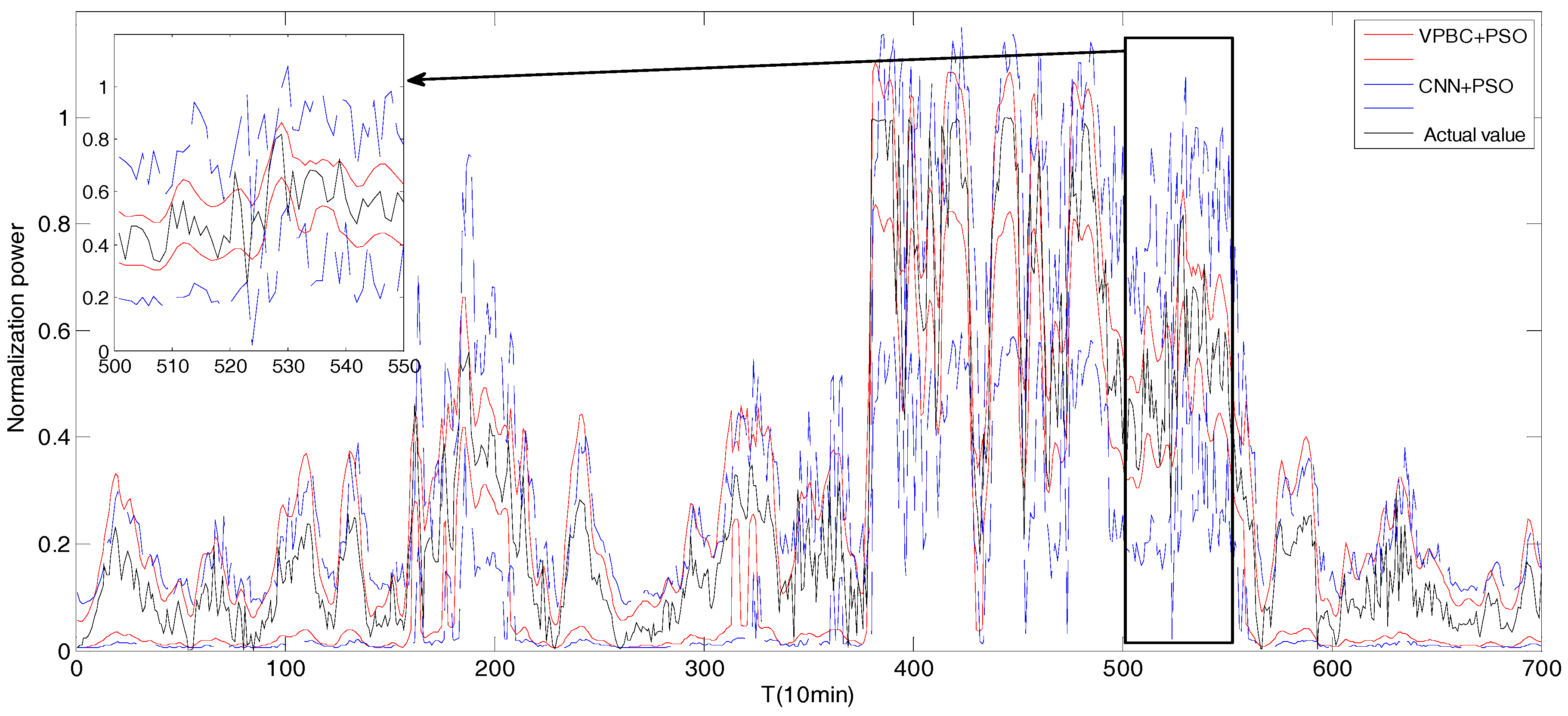
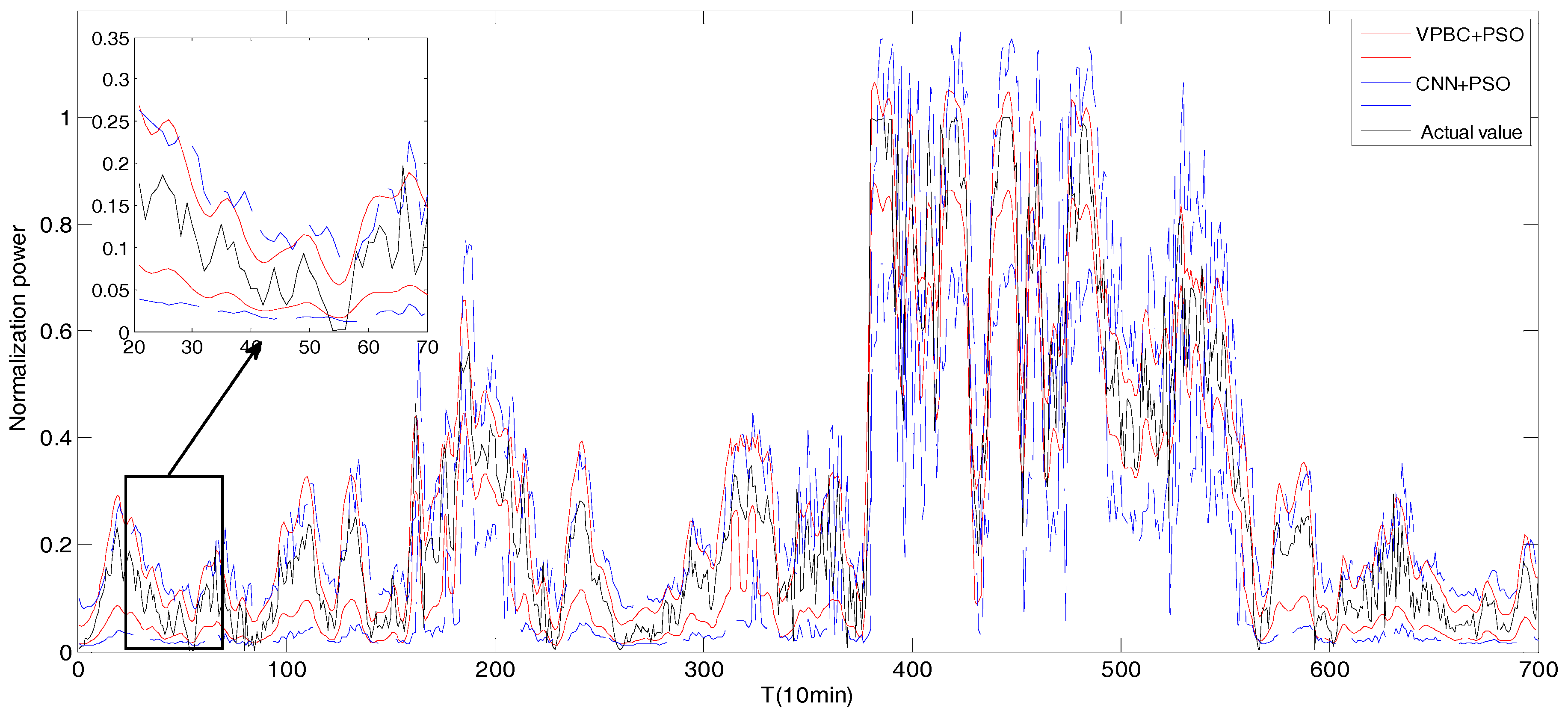
| VPBC + PSO | 85.14% | 0.1371 | 87.86% | 0.1587 | 91.86% | 0.1876 |
| VPCB + PSO | 81.29% | 0.1521 | 85.43% | 0.1725 | 89.57% | 0.2041 |
| CNN + PSO | 83.71% | 0.2182 | 86.00% | 0.2477 | 90.14% | 0.2885 |
| Method | PINC 80% | PINC 85% | PINC 90% | |||
|---|---|---|---|---|---|---|
| PICP | PINAW | PICP | PINAW | PICP | PINAW | |
| VPBC + PSO | 85.14% | 0.1371 | 87.86% | 0.1587 | 91.86% | 0.1876 |
| VPBC + GA | 83.86% | 0.1381 | 86.29% | 0.1624 | 91.14% | 0.1880 |
| Method | NMAE | NRSME | MAPE |
|---|---|---|---|
| VPBC | 1.39% | 0.2548 | 2.65% |
| CNN | 3.14% | 0.3295 | 5.97% |
| VPCB | 2.10% | 0.2686 | 3.99% |
| Persistence | 1.42% | 0.2313 | 2.69% |
© 2019 by the authors. Licensee MDPI, Basel, Switzerland. This article is an open access article distributed under the terms and conditions of the Creative Commons Attribution (CC BY) license (http://creativecommons.org/licenses/by/4.0/).
Share and Cite
Yang, X.; Zhang, Y.; Yang, Y.; Lv, W. Deterministic and Probabilistic Wind Power Forecasting Based on Bi-Level Convolutional Neural Network and Particle Swarm Optimization. Appl. Sci. 2019, 9, 1794. https://doi.org/10.3390/app9091794
Yang X, Zhang Y, Yang Y, Lv W. Deterministic and Probabilistic Wind Power Forecasting Based on Bi-Level Convolutional Neural Network and Particle Swarm Optimization. Applied Sciences. 2019; 9(9):1794. https://doi.org/10.3390/app9091794
Chicago/Turabian StyleYang, Xiyun, Yanfeng Zhang, Yuwei Yang, and Wei Lv. 2019. "Deterministic and Probabilistic Wind Power Forecasting Based on Bi-Level Convolutional Neural Network and Particle Swarm Optimization" Applied Sciences 9, no. 9: 1794. https://doi.org/10.3390/app9091794
APA StyleYang, X., Zhang, Y., Yang, Y., & Lv, W. (2019). Deterministic and Probabilistic Wind Power Forecasting Based on Bi-Level Convolutional Neural Network and Particle Swarm Optimization. Applied Sciences, 9(9), 1794. https://doi.org/10.3390/app9091794