Abstract
The application of the micro-electro-mechanical system inertial measurement unit has become a new research hotspot in the field of inertial navigation. In order to solve the problems of the poor accuracy and stability of micro-electro-mechanical system sensors, redundant design is an effective method under the restriction of current technology. Redundant data processing is the most important part in the micro-electro-mechanical system redundant inertial navigation system, which includes the processing of anomaly data and the fusion estimation of redundant data. To further improve the reliability of the micro-electro-mechanical system redundant inertial measurement unit, an anomaly detection, isolation, and recognition method for data anomalies is proposed. The relationship between the parity space method detection function and the deterioration degree of anomaly data is mathematically deduced. The parity space method detection functions of different anomalies are analyzed, and five indicators are designed to quantitatively analyze the detection function values. According to these indicators, the detection and recognition method are proposed. The new method is tested by a series of simulation experiments.
1. Introduction
Micro-electro-mechanical system inertial measurement unit (MEMS IMU) has the advantages of being low cost, small volume, and lightweight, but low precision and poor stability are still problems that cannot be ignored. Many aircraft, cars, and satellites are beginning to use MEMS sensors [1,2,3,4,5]. Among them, most MEMS accelerators have already met the tactical and navigation grade requirements [6,7]. However, only a few MEMS gyros can reach the level of tactical grade [1], and these tactical grade gyros are too expensive for common application. To improve the performance of MEMS IMU, a series of studies have been conducted to promote MEMS manufacturing technology. On the other hand, the improvement can also be achieved through reasonable designs and algorithms.
Under the restriction of current manufacturing technology, a lot of research has been done to improve the performance of the MEMS system, and redundant design is the most effective approach to improve the accuracy and stability [8,9,10,11,12,13]. Even for the tactical or navigation grade sensors, the redundant configuration can improve the performance substantially [14]. In the redundant inertial navigation system (RINS), the processing of redundant data is the most important link. It is divided into two parts: processing data anomalies and fusing redundant data. The motivation of this paper is to develop the anomaly diagnosis method, and improve the reliability of the MEMS RINS.
The data anomalies are comprised of sensor faults and outliers. The faults refer to the failure and variation of sensor characteristics, which are probably caused by harsh environmental conditions, such as the moisture, extreme temperature, electromagnetic radiation, impact, and vibration [15]. These kind anomalies are related to the aging, damage, and performance degradation of the sensors, and they are generally irreversible hard failures. The definition of an outlier is an observation (or subset of observations) which appears to be inconsistent with the remainder of that set of data. The outliers in inertial measurement data arise because of instrument error, natural deviations, or changes in the behavior of systems. The outliers usually appear as the self-recovery and transient mutations [16].
For further analysis, the anomalies can be divided into more subcategories based on a different baseline. In this paper, anomaly patterns serve as evidence to choose anomaly solution methods. So we classify anomalies as short-duration auto-recovery anomalies and sustained anomalies. The former includes isolated outliers, small outlier patches, transient faults, etc., which refer to the anomalies that sustain a short duration and recover spontaneously. The short-duration auto-recovery anomalies can be corrected well with outlier eliminating methods. The latter includes large outlier patches, hard faults, permanent failures, etc. These kinds of anomalies can be subdivided by their different performance characteristics. The constant drift fault and multiplicative fault (variation of scale factor) can be repaired through re-calibration technology [17,18]. For instance, the faulty sensors can be calibrated with the data of other types of navigation information or the fusion estimation signal without anomaly data. However, large outlier patches, noise failure, complete failure, and other hard faults are usually isolated directly. Overall, the reclassification of anomalies is shown in Figure 1.
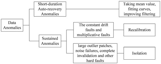
Figure 1.
The classification of data anomalies.
At present, most methods only divide the anomalies into faults and outliers to process. Due to the differences between faults and outliers, the countermeasures against them are carried out separately in different ways. To protect the output fusion signal from faults, the fault detection and isolation (FDI) methods can make the system continue working normally [19,20,21,22]. The solution against the faults is to detect the measurement data in real time, isolate faulty sensors and discontinue using them. A set of FDI methods have already been applied in the RINS successfully, which includes the Chi-square test [23,24], the network-based method [25], and the parity space method. The parity space method includes the optimal parity vector test (OPT) [26], the generalized likelihood test (GLT) [27,28], and the singular value decomposition (SVD) method [21,22,29,30,31]. Among these methods, the methods based on the Chi-square test are subjected to the filtering algorithm performance. When the filtering performance is degraded or even diverged, the detection and isolation results are not reliable. The neural network-based methods are restricted by the heavy computing burden and the requirements for large samples. In the main, the parity space method is a good choice for the navigation system, but it cannot handle the situation of multi faults. As for the outliers, there are two approaches commonly used to deal with them: one is to improve filter functions, which alleviate the impact of outliers by setting the weighted matrix or correcting the covariance matrix at every sampling moment [32,33,34,35]; another one is to replace the detected outlier points with mean values or the points from fitted curves [36,37].
The methods introduced above can reduce the effect of anomalies to some degree, but there are still some problems. Firstly, the outliers in the measurement data, especially the outlier patches, are easily misdiagnosed as the faults, which will lead to an increase in the false alarm rate. The outliers will cause the detection function values to exceed the detection threshold, but there is no failure or damage in the sensor with outliers. Such misdiagnosis may induce a well-behaved sensor to be deactivated. Secondly, when the outlier eliminating methods and FDI methods are operating simultaneously, the practical performance may degrade, because the calculation burden will increase and the results of different methods will interfere with each other. For example, the outlier eliminating methods regard every anomaly point as an outlier. Since the deviation of anomaly points caused by sensor faults will be diminished after the outlier eliminating processing, the original statistical characteristics of the faults will change. As a result, the probability of correct detection (PCD) and the probability of correct isolation (PCI) will decline. Thirdly, the FDI methods cannot identify the patterns of anomalies. So the different modes of anomalies have to be handled in the same way. Deactivating sensors with hard faults is reasonable. However, some faulty sensors are not physically damaged and can continue to be used after correction, so traditional strategies can possibly result in the loss of available sensors.
To solve the problems above, this paper proposed a diagnosis method for data anomalies in MEMS RINS. The SVD-based method is briefly reviewed, and the flaws of this method are analyzed. The improved SVD-based method is presented. The disadvantages of this method are analyzed and improved. To demonstrate the feasibility of recognizing a fault pattern by analyzing the detection function, the mathematical relation between the detection function and sensor faults is derived. Five indicators of detection are defined on the basis of the analysis of various anomalies. The anomaly recognition method is proposed according to these five indicators. The proposed method can detect faults and outliers simultaneously, so that, the mutual interference between outlier eliminating and fault detection can be removed. The anomalies can receive suitable and reasonable treatments based on the recognition results. The anomaly processing is simplified too.
This paper is organized as follows: In Section 2, the SVD method is briefly reviewed, and the disadvantages are discussed and improved. To demonstrate the feasibility of using detection function values as the evidence for anomaly recognition, the relation between the detection function and anomalies is deduced. In Section 3, the five indicators are designed to analyze different anomalies quantitatively, and the anomaly detection and recognition method are presented. In Section 4, the simulation experiments are conducted to test the proposed method. Section 5 gives the conclusion.
2. The Detection and Isolation Method of the Parity Space Method
2.1. The SVD-Based Method and Improvement
The parity space method is a diagnosis method based on analytic redundancy. Its basic idea is to construct a parity matrix based on the hardware redundancy or analytical redundancy equation of the system, and use the actual observation to check the parity (consistency) of the system mathematical model (analytic redundancy relationship). The method needs to find the parity equation decoupled from the faults, and then the parity vector and the fault detection function are constructed based on the parity equation. With the detection threshold determined by hypothesis testing theory, the faults can be detected once the detection function values exceed the threshold. In this paper, the SVD-based method [22] is used as an example to deduce the relation between detection functions and data anomalies. This relation is the basis to analyze anomalies.
In normal working, the observation equation of a redundant system composed of n gyroscopes can be expressed as follows:
In the equation, Z is the measurement data vector of n-dimensional; is the geometric configuration matrix; is the n-dimensional white Gaussian noise vector which statistical characteristics meet:
When the anomalies appear, the observation equation can be expressed as:
In Equation (3), b is the anomaly vector. Several typical anomaly vectors are described in Table 1.

Table 1.
The anomaly vectors of several typical anomalies.
Note that, “Duration” refers to the number of sampling points from the anomaly appearing to the disappearing; “N” is the number of sampling points in a single diagnostic period; “\” indicates that the anomalies vectors are not fixed or too difficult to express by mathematical equation; dio is the outlier vector; e is the white noise vector with zero mean value; d is the constant drift vector with fixed values of each element; is the anomaly coefficient matrix with fixed values of each element. is also a diagonal matrix, and the elements of normal sensors at the diagonal line equal to zero.
To detect anomalies, in [22], an SVD-based method was presented and a detailed derivation and verification was conducted. The first step is to decompose the geometric configuration matrix H through singular value decomposition.
In Equation (4), the matrix SH is a diagonal matrix. The decoupling matrix V is constructed from the matrix as follows:
where and .
The parity vector is calculated with the matrix V and the measurement vector as follows:
In [22] the fault detection function and isolation function are constructed as follows:
where the Vi is the fault reference vector, which refers to the i-th column of the matrix V, and the corresponds the i-th sensor. The decision rule to detect fault is given as follows:
In [22], it is suggested that the FD obeys the distribution, so the threshold TD can be determined with a given false alarm probability . If H0, then the system can be considered fault-free; if H1, then proceed to the isolation step. The fault isolation function of each sensor is calculated out. Next, the largest isolation function is found and the k-th sensor is isolated.
2.2. The Improvement of the SVD-Based Method
The method above has the following disadvantages, which are analyzed and proved in [31]:
- (1)
- The detection function has the probability to disobey the distribution, because the distribution requires that each variable is independent. The matrix V is singular, so elements of the vector are not independent. As a result, the threshold determined by distribution is inappropriate.
- (2)
- The isolation function given in Equation (9) may cause the inequality of isolation probability among the sensors. The isolation function is designed to indicate the similarity between the parity vector and the fault reference vector, and the sensor with the highest similarity is most likely to get faulty. From Equation (9), the values of isolation function are subjected to the modules of Vi, but there is no guarantee that the modules of each fault reference vector Vi are equal. The similarity between two vectors is supposed to only depend on the projection or the angular between them. In other words, the modules of fault reference vectors are not supposed to influence the isolation function. A more appropriate method is to use the angular between the parity vector and the fault reference vector Vi. For example, consider a simple situation: , and . Calculate the isolation function values with Equation (9), and there are and . So the result of the original method is that the first senor is faulty. However, the angular between and is 30°, and the angle between and is 60°. It is obvious that the second sensor is most likely to have faults, and the original method produced an incorrect result.
- (3)
- The isolation strategy is flawed as it cannot isolate the negative faults. For example, we simulate a set of measurement signals based on 6-gyros-dodecahedron redundant system. A positive step fault and a negative fault are injected in the fourth gyro in turn. The signal, detection function, and isolation function are shown in Figure 2. Analyzing the figure, the detection function is able to detect the faults once the faults are injected. But the isolation strategy chooses the sensor to isolate, which corresponds to the largest isolation function value; however, the negative fault will bring down the isolation function values of the faulty sensor. So the isolation function fails to isolate negative faults.
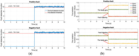 Figure 2. The fault detection and isolation function in two cases: (a) The detection functions of positive fault and negative fault; (b) The isolation functions of positive fault and negative fault.
To solve the problems above, the method is improved as follows: To solve the first problem, the decoupling matrix V is redefined and the parity vector is standardized as follows:
Since this improvement, the obeys distribution, and the threshold can be determined with a given false alarm rate .
To solve the last two problems, the isolation function is redefined as follows:
The improved isolation function indicates the angular between the parity vector and the i-th fault reference vector Vi, and the effect of the module of Vi is eliminated. Therefore, the imparity caused by the difference of modules of fault reference vectors will not influence the isolation results. The negative-fault problem can also be solved through the squaring operation in Equation (13).
2.3. The Relation Between Detection Function and Anomaly Vector
In Section 3, the anomaly recognition method is proposed, and the method is based on the analysis of the detection function. To verify the feasibility of the proposed method, the relation between the detection function and the anomaly vector is deduced here. Take (3), (6), and (7) into (8), and the detection function is given as follows:
The singular value decomposition of is given by
where .
Compared with Equation (4), the relations can be expressed as follows:
Further, we can deduce out that , . Equations (4) and (15) can be simplified as
The null space of the matrix is , and it can be expressed as
is a non-singular matrix. From the conclusion of SVD, there is , so is equivalent to . Equation (18) can be simplified as
Because is an orthogonal matrix, the solution space of is the range of the column vectors of , which is . Consequently, the equations are established as follows:
From Equation (21), it is concluded that . The detection function can be simplified as
Because is an orthogonal matrix, and each column vector is a unit vector, the column vectors of are orthogonal to each other. Then another equation can be given by
Taking Equations (11) and (16) into (23), the relation above can be expressed as
The error vector and noise vector can be replaced by
So the detection function is expressed as follows:
Since the obeys the Chi-square distribution, the variation of that exceeds the threshold can be thought to be caused by the anomaly vector b. The anomaly vectors b for various types of data anomalies are definitely different, so the distributions and variation trends of also differ. The patterns of data anomalies can be identified by analyzing the detection function.
3. The Detection and Isolation Method of Data Anomalies
3.1. Simulation and Analysis of Anomaly Signal
To demonstrate the differences among the anomalies, a set of gyro measurement signals are simulated, and six typical anomalies given in Table 1 are injected into those signals. The dynamic gyro signal generator is built by Simulink (shown in Figure 3). The gyro redundant unit uses 6-gyro-dodecahedron configuration. The simulation only considers two main random noises, angle random walk (ARW) and rate random walk (RRW), and the determinate error and other random noise are ignored. The sampling time is 100 s; sampling frequency is 100 Hz. The frequency of the sinusoidal signal is Hz; the amplitude is 10°/s. The false alarm rate is 1%; the detection threshold is 16.812; and .
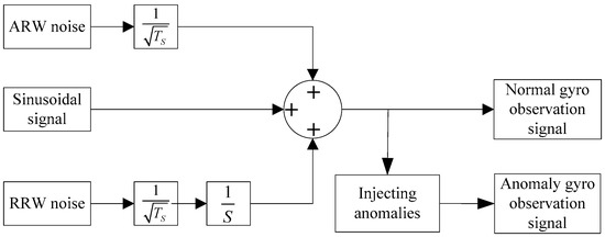
Figure 3.
Gyro signal generator.
Several typical anomalies are injected into the original signal in turn (shown in Figure 4). Among them, the isolated outliers, outlier patches, and transient faults are injected into normal observation signals every 10 s. The noise faults, constant drift faults, and multiplicative faults are injected at 50th second. The amplitudes of isolated outliers and outlier patches are a series of random numbers greater than , and the amplitudes of transient faults are a series of random numbers greater than . The parameters of constant drift fault, noise fault, and multiplicative fault are fixed in each turn, and the parameters are given by , ; ; .
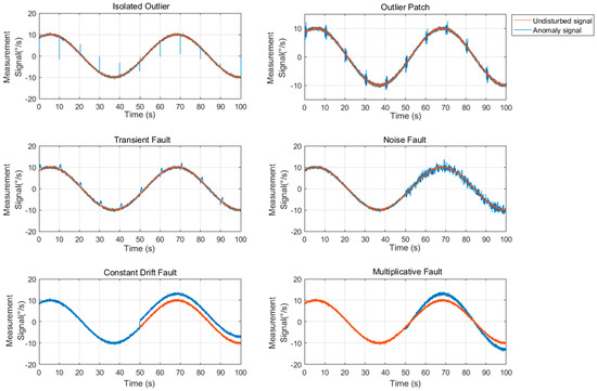
Figure 4.
Gyro simulation signals.
The diagnosis period N is introduced here. The definition of diagnosis period refers to the number of sampling points in the duration from the first moment when the detection function exceeds the threshold to the moment to get the diagnosis result. The data during the period is analyzed to recognize the anomaly mode. It is important to take a suitable diagnosis period. If the period is too short, the information is not enough to get accurate recognition results. Conversely, an unduly long period will lead to a delay, and cause the diagnosis sensitivity to decrease.
The SVD-based method is used to detect those signals. The detection function is shown in Figure 5a. Figure 5b shows the detection function values in a single diagnosis period. The diagnosis period N is 100, and the X-axis represents the number of sampling points. Note that, in Figure 5, the red line is the detection threshold, and the blue line represents the detection function. Once the blues line exceeds over the red line, it can be considered that the anomalies appear.
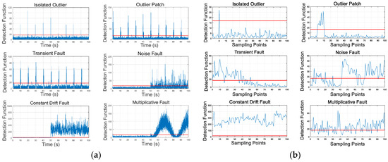
Figure 5.
(a) Detection function of different anomalies; (b) detection function of different anomalies in a single diagnosis period.
As Figure 5a shows, the improved method has several useful features of the fault detection: First, the detection function values exceed the detection threshold whenever data anomalies occur; second, the values and trends of the detection function are consistent with the anomalies deterioration degree. Because of the consistency between anomalies and detection function, analyzing detection function is an eligible approach for anomaly recognition.
From inspection of Figure 5b, the detection function values of different anomalies present different distributions and trends in a single diagnosis period. The diversity among different anomaly modes is the key to recognize them. For the distributions, detection functions of short-duration auto-recovery anomalies exceed the threshold fewer times, while the detection functions of sustained anomalies exceed the threshold more times for its longer durations. On the other hand, the anomaly points of short-duration auto-recovery anomalies only make up a small part, and they deviate seriously from the trend than other normal points present. However, for sustained anomalies, the anomaly points take up large proportions, so the trend of normal points is indistinct and unstable. Concerning the variation trend, the short-duration auto-recovery anomalies present the decreasing trend when the anomalies disappear. For the sustained anomalies, the detection function values of the multiplicative fault are proportional to the absolute values of the actual measurement data, and there is no definite trend of the noise fault or of the constant drift fault.
3.2. The Indicators
According to the analysis above, five indicators are proposed to indicate the characteristics of anomaly signals.
3.2.1. The Proportion of Error Points
The proportion of error point r refers to the ratio of points whose detection function exceeds the threshold to the total sampling points in a single diagnosis period. The calculation formula of r is defined as follows:
3.2.2. The Mutation Degree
The mutation degree h reflects how serious the mutation points derail the trend of normal points. The values of h grow larger when the mutations exist in measurement data, and h is proportional to the deviation degree.
The nk is the number of points which detection function values stay in the rage of Nk.
3.2.3. The Recovery Trend Indicator
The recovery trend indicator reflects the numerical relation between the predicted at the end of the next period and the detection threshold. If , the predicted values of will exceed the threshold, which means the probability is tiny for anomalies to disappear. Instead, if , the predicted values of will be lower than the threshold, which means anomalies are likely to disappear, and the greater g means greater probability.
First, the detection function values in the period are taken with 0.1 s averaging, so there are n average values of detection function in each period. Then fit the through the least-square polynomial fitting method:
In Equation (32), those matrices are given by
Thus, the estimate equation is expressed as
The new statistics can be defined as follows:
where
3.2.4. The Mean-Value-Crossing Rate
The mean-value-crossing rate v is the rate of changes in the size relation between detection function values and their averages. As Figure 3 shows, noise faults and constant drift faults can be regarded as random series with a fixed arithmetic mean. The detection function values randomly float near the mean, so the values of v of these anomalies are relatively higher. As for the kind of transient-type anomalies, they keep a fixed trend to change, so the values of v are relatively lower.
where
3.2.5. The Proportional Coefficient Variance
With regard to multiplicative faults, the distribution and variation of the detection function values are determined by the actual state. Hence, the indicators proposed above cannot achieve good recognition results. The proportional coefficient variance DK is to measure whether the ratio of observation data to the actual measurement data is stable, which is mainly used to identify the multiplicative fault. That ratio will stabilize near a certain constant value in the case of multiplicative faults, so the DK is small; conversely, the other kinds of anomalies cannot keep a stable ratio, so the DK gets larger.
As for multiplicative faults, the observation equation and the error vector are given by
The detection function becomes
From Equation (45), the relationship between the detection function and actual state is derived as
where the xk is the real state values, which can be taken the place by the filter estimates. Let , and the proportional coefficient variance DK is the variance of ke. The calculating equation is given by
3.3. The Recognition Method for Data Anomalies
The five indicators above are taken as evidence to recognize the anomaly patterns. The logical order of recognition is shown in Figure 6.
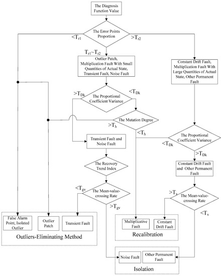
Figure 6.
Logical order of data anomalies pattern recognition.
4. Simulation Experiments
In this section, a set of simulation experiments are conducted to verify the performance of the proposed method. In Section 4.1, the ability of each indicator to separate different anomalies is demonstrated. In Section 4.2, the detection and recognition performance of the method for various faults is verified. In Section 4.3, to demonstrate the advantages, the new strategy is compared with the old in various conditions.
Due to the limitation of the MEMS gyro structure, a large number of anomaly samples of a certain mode are difficult to obtain in practical experiments. Referring to other relevant literature [22,26,27], the signals from the practical experiment are injected with simulation anomaly signals. The following experiments use these signals as samples to test the performance of the new method. Gyro redundant unit adopts the 6-gyros-dodecahedron configuration. The rolling motion signal is generated from a three-axis turntable; the sampling time is 600 s; sampling frequency is 100 Hz. The frequency of the rolling motion signal is Hz; the amplitude is 15°/s. The output signal and residual value of a single gyro are shown in Figure 7.
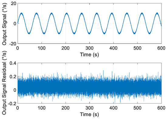
Figure 7.
The output signal and residual value of a single gyro.
4.1. The Simulation Experiments of Indicators
Based on the simulation settings above, 100 sets of simulation signals of each type anomaly are generated as samples to test the performances of indicators and calculate the boundaries. Every set of simulation signals has only one anomaly with the random amplitude, and the time when the anomalies occur is random too. For the constant drift fault, noise fault, and multiplicative fault, the anomaly parameters d, e, and Ke are fixed in a single simulation.
According to Figure 6, the first step is to use the proportion of error points r to analyze the detection function. The details of different anomalies are shown in Figure 8 and Table 2. The boundary thresholds, Tr1 and Tr2, are calculated by the genetic algorithm and equal to 0.186 and 0.936, respectively. The anomalies can be treated as false points or outliers once r is under Tr1; the anomalies may be outlier patches, multiplicative faults in a low dynamic situation, transient faults, or noise faults, once r is between Tr1 and Tr2; the anomalies may be constant drift faults, multiplication faults in a dynamic situation, or other permanent hard faults once r exceeds over Tr1.
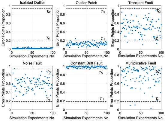
Figure 8.
The distribution of the proportion of error points in different situations.
Table 2.
The distribution of the proportion of error points in different situations.
Firstly, we analyze the situations where r is between Tr1 and Tr2. In this kind of situation, the second step is to identify the multiplicative faults. The distribution of DK of transient faults, noise faults, constant drift faults, and multiplicative faults are shown in Figure 9 and Table 3. The boundary threshold TDk calculated by the genetic algorithm is 0.0552. The anomalies can be regarded as multiplicative faults once DK is under TDk. In Figure 9, the Y-axis range is from 0 to 0.9. Besides, for other anomaly types, some values of Dk are greater than 0.9 and up to , which are not drawn in the figure.
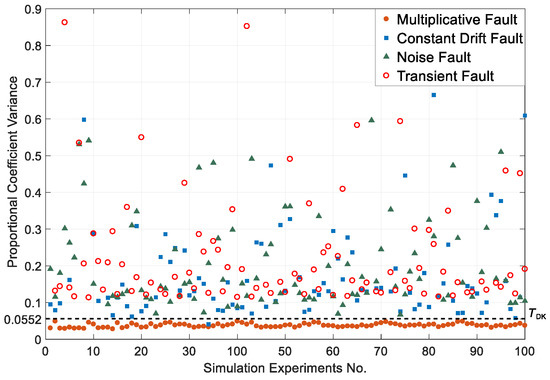
Figure 9.
The distribution of the proportional coefficient variance of different anomalies.
Table 3.
The distribution of the proportional coefficient variance of different anomalies.
When the real state values are small, the values of r in multiplicative faults are close to outlier patches. For the outlier patches, normal points take a larger part in the diagnosis period, so the ratio of measurement data to real values fluctuates around 1. As a result, the DK will also remain at a low level. It is difficult to distinguish the multiplicative faults and outlier patches in such a situation. The mutation degree is designed to solve this problem. The distributions of the mutation degree of multiplicative faults and outlier patches are shown in Figure 10 and Table 4. The boundary threshold Th calculated by the genetic algorithm is 58.83. The anomalies can be regarded as outlier patches once the mutation degree exceeds over Th.
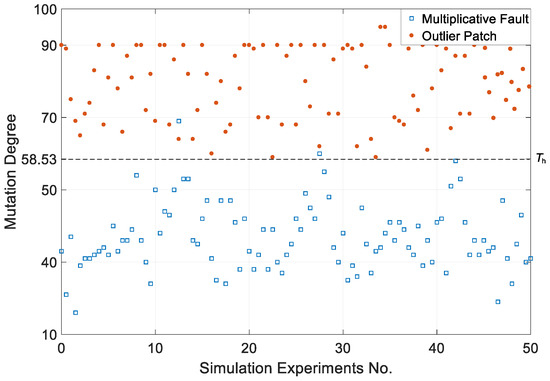
Figure 10.
The distribution of the mutation degree of different anomalies.
Table 4.
The distribution of the mutation degree of different anomalies.
The last step is to distinguish transient faults and noise faults through the recovery trend index and the mean-value-crossing rate. The distribution is shown in Figure 11 and Table 5. The boundary obtained by linear SVM is . The transient faults are above the boundary line, and the noise faults are under the line.

Figure 11.
The distribution of transient faults and noise faults.
Table 5.
The distribution of transient faults and noise faults.
Next, we analyze the situations where r exceeds the Tr2. In this kind of situation, the multiplicative faults are identified firstly by DK, which is the same as the situation discussed above. Constant drift faults are then identified by mean-value-crossing rate. In a single diagnosis period, the observation errors of constant drift faults are stable. As a result, the detection function values can be seen as a random series with fixed mean. Because of this feature, the mean-value-crossing rate v is high. Considering complete faults (the observation data is identically equal to 0 or other values) and other permanent faults, the error is not constant, so the mean-value-crossing rate is lower. The boundary threshold Tv between constant drift faults and 100 sets of complete faults is 37.16%, and the distributions are shown in Figure 12 and Table 6.
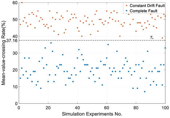
Figure 12.
The distribution of the mean-value-crossing rate of constant drift faults and complete faults.
Table 6.
The distribution of the mean-value-crossing rate of constant drift faults and complete faults.
4.2. The Simulation and Analyzing for Anomaly Detection and Recognition Method
In the above, the simulation experiments are conducted to verify the ability of each indicator to separate different anomalies. This part is to test the diagnosis performance of the proposed method. To conduct the Monte Carlo simulation test, the isolated outliers, outlier patches, transient faults, noise faults, constant drift faults, and multiplicative faults are injected into the original observation data 500 times for each type. In each simulation experiment, only one anomaly is injected into the normal signal, and the injection moment is random. Other simulation conditions and parameters are the same as in Section 4.1.
The probability of correct detection (PCD) and the probability of correct recognition (PCR) are counted out and shown in Table 7. From Table 7, the PCD and PCR of the new method can both reach a high level. We can conclude that the proposed method is capable of anomaly diagnosis.
Table 7.
Simulation experiment statistics of the new method.
4.3. The Comparison and Analyzing of Different Methods
For comparison, the simulation signals are diagnosed through current outliers eliminating methods and FDI methods, and the results are shown in Table 8. The detection methods used for comparison include 3 criterion-based method [36], Grubbs criterion-based method [37], GLT-method [27], OPT-based method [26], and Chi-square-based method [23]. Comparing Table 8 and Table 7, the PCD of the proposed method remains slightly higher than previous methods.
Table 8.
Simulation experiment statistics of the traditional method.
Running outlier eliminating methods and FDI methods at the same time will decrease the PCD, but there is no such problem in the new method. To verify this, two approaches are conducted to diagnose transient faults, noise faults, constant drift faults, and multiplicative faults: the first one is that outlier points are marked at first through Grubbs criterion and replaced by the points calculated through cubic spline interpolation method [35], then the processed signal will be diagnosed by several current FDI methods; the second way is to use the new method directly. The FDI methods used in the first strategy include the GLT-based method [27], OPT-based method [26], and Chi-square based-method [23].
The experiment results are shown in Table 9. As the table shows, the outlier eliminating does reduce the PCD of FDI method, because the outlier eliminating methods regard every error point as the outlier, which will cause the deviation degree of error points greatly decrease, so that some faults may be missed.
Table 9.
Statistics of diagnostic results of different methods after outliers eliminating.
5. Conclusions
In this paper, an anomaly diagnosis method for RINS is proposed. The features of different anomaly signals are analyzed, and five indicators are designed base on these features. These five indicators reflect the characteristics of the main aspects of the measurement signals. The new method monitors the observation data of RIMU and identifies anomalies with the proposed five indicators. In this paper, the simulation signals with anomalies serve as samples to test the proposed method. Experiments prove that the detection performance of the proposed method is better than the previous FDI methods. Further, our proposed method can identify the specific anomaly types. Based on the recognition results of this paper, the different anomalies can be identified and handled in a more reasonable way. At the same time, this method can solve interaction between the outlier eliminating algorithms and FDI technologies. Both the reliability and stability of RIMU can be improved.
Due to the manufacturing technology and the structure of MEMS, the MEMS sensors are packaged during the manufacturing. It is difficult to set practical faults artificially on the sensors, so plenty of typical sample data is hard to collect. As a result, the theories of statistical learning are not applicable to MEMS RINS. Besides, the proposed anomaly recognition method also needs more practical samples to test. These issues remain to be resolved in future research.
Author Contributions
B.D.: Conceptualization, Formal analysis, Writing—original draft; J.S.: Conceptualization, Supervision, Writing—review and editing; Z.S.: Conceptualization, Supervision, Writing—review and editing, funding acquisition.
Funding
This research received no external funding.
Conflicts of Interest
The authors declare no conflict of interest.
References
- Passaro, V.; Cuccovillo, A.; Vaiani, L.; De Carlo, M.; Campanella, C.E. Gyroscope technology and applications: A review in the industrial perspective. Sensors 2017, 17, 2284. [Google Scholar] [CrossRef]
- Lin, T.; Zhang, Z.; Tian, Z.; Zhou, M. Low-Cost BD/MEMS Tightly-Coupled Pedestrian Navigation Algorithm. Micromachines 2016, 7, 91. [Google Scholar] [CrossRef]
- Navidi, N., Jr.; Landry, R.; Cheng, J.; Gingras, D. A new technique for integrating mems-based low-cost imu and gps in vehicular navigation. J. Sens. 2016, 2016, 5365983. [Google Scholar] [CrossRef]
- Dichev, D.; Koev, H.; Bakalova, T.; Louda, P. A gyro-free system for measuring the parameters of moving objects. Meas. Sci. Rev. 2014, 14, 263–269. [Google Scholar] [CrossRef]
- Zhou, S.; Fei, F.; Zhang, G.; Mai, J.D.; Liu, Y.; Liou, J.Y.; Li, W.J. 2d human gesture tracking and recognition by the fusion of mems inertial and vision sensors. IEEE Sens. J. 2014, 14, 1160–1170. [Google Scholar] [CrossRef]
- Hopkins, R.; Miola, J.; Setterlund, R.; Dow, B.; Sawyer, W. The silicon oscillating accelerometer: A high-performance MEMS accelerometer for precision navigation and strategic guidance applications. In Proceedings of the 61st Annual Meeting of The Institute of Navigation, Cambridge, MA, USA, 27–29 June 2005. [Google Scholar]
- Becka, S.; Novack, M.; Slivinsky, S.; Paul, C. A High Reliability Solid State Accelerometer for Ballistic Missile Inertial Guidance. In Proceedings of the AIAA Guidance, Navigation and Control Conference and Exhibit, Honolulu, HI, USA, 18–21 August 2008; p. 7300. [Google Scholar]
- Chadli, M.; Maquin, D.; Ragot, J. Static output feedback for Takagi-Sugeno systems: An LMI approach. In Proceedings of the 10th Mediterranean Conference on Control and Automation, MED’2002, Lisbonne, Portugal, 9–12 July 2002. [Google Scholar]
- Chadli, M.; Maquin, D.; Ragot, J. Nonquadratic stability analysis of Takagi-Sugeno models. In Proceedings of the 41st IEEE Conference on Decision and Control, Las Vegas, NV, USA, 10–13 December 2002; Volume 2, pp. 2143–2148. [Google Scholar]
- Jafari, M.; Roshanian, J. Optimal redundant sensor configuration for accuracy and reliability increasing in space inertial navigation systems. J. Navig. 2013, 66, 199–208. [Google Scholar] [CrossRef]
- Nilsson, J.O.; Skog, I. Inertial sensor arrays—A literature review. In Proceedings of the 2016 European Navigation Conference (ENC), Helsinki, Finland, 30 May–2 June 2016; pp. 1–10. [Google Scholar]
- Cheng, J.; Dong, J., Jr.; Landry, R.; Chen, D. A Novel Optimal Configuration form Redundant MEMS Inertial Sensors Based on the Orthogonal Rotation Method. Sensors 2014, 14, 13661–13678. [Google Scholar] [CrossRef] [PubMed]
- Luo, Z.; Liu, C.; Yu, S.; Zhang, S.; Liu, S. Design and analysis of a novel virtual gyroscope with multi-gyroscope and accelerometer array. Rev. Sci. Instrum. 2016, 87, 085003. [Google Scholar] [CrossRef] [PubMed]
- Jafari, M.; Najafabadi, T.A.; Moshiri, B.; Tabatabaei, S.S.; Sahebjameyan, M. Pem stochastic modeling for mems inertial sensors in conventional and redundant imus. Ieee Sens. J. 2014, 14, 2019–2027. [Google Scholar] [CrossRef]
- Huang, Y.; Vasan, A.; Doraiswami, R.; Osterman, M.; Pecht, M. Mems reliability review. IEEE Trans. Device Mater. Reliab. 2012, 12, 482–493. [Google Scholar] [CrossRef]
- Hodge, V.J.; Austin, J. A survey of outlier detection methodologies. Artif. Intell. Rev. 2004, 22, 85–126. [Google Scholar] [CrossRef]
- Wang, Z.W.; Qin, J.Q.; Yang, G.L. Sins field calibration based on BD II differential positioning. Aerosp. Sci. Technol. 2016, 62, 108–113. [Google Scholar] [CrossRef]
- Xie, L.; Lu, J. Optimisation-based transfer alignment and calibration method for inertial measurement vector integration matching. J. Navig. 2017, 70, 595–606. [Google Scholar] [CrossRef]
- Chibani, A.; Chadli, M.; Ding, S.X.; Braiek, N.B. Design of robust fuzzy fault detection filter for polynomial fuzzy systems with new finite frequency specifications. Automatica 2018, 93, 42–54. [Google Scholar] [CrossRef]
- Li, L.; Chadli, M.; Ding, S.X.; Qiu, J.; Yang, Y. Diagnostic observer design for t–s fuzzy systems: Application to real-time-weighted fault-detection approach. IEEE Trans. Fuzzy Syst. 2018, 26, 805–816. [Google Scholar] [CrossRef]
- Shim, D.S.; Yang, C.K. Optimal configuration of redundant inertial sensors for navigation and FDI performance. Sensors 2010, 10, 6497–6512. [Google Scholar] [CrossRef]
- Shim, D.S.; Yang, C.K. Geometric FDI based on SVD for redundant inertial sensor systems. In Proceedings of the 2004 5th Asian Control Conference (IEEE Cat. No. 04EX904), Melbourne, Australia, 20–23 July 2004; Volume 2, pp. 1094–1100. [Google Scholar]
- De Oliveira, É.J.; da Fonseca, J.M. Fault detection and isolation in inertial measurement units based on -CUSUM and wavelet packet. Math. Probl. Eng. 2013, 2013, 1–10. [Google Scholar] [CrossRef]
- Zhang, H.Q.; Li, D.X.; Zhang, G.Q. Application of hybrid chi-square test method in fault detection of integrated navigation system. J. Chin. Inert. Technol. 2016, 5, 142–146. [Google Scholar]
- Liu, C.; Wang, H.; Li, N.; Yu, Y. Sensor Fault Diagnosis of GPS/INS Tightly Coupled Navigation System Based on State Chi-square Test and Improved Simplified Fuzzy ARTMAP Neural Network. In Proceedings of the 2017 IEEE International Conference on Robotics and Biomimetics (ROBIO), Macau, China, 5–8 December 2017; pp. 2527–2532. [Google Scholar]
- Jin, H.; Zhang, H.Y. Optimal parity vector sensitive to designated sensor fault. IEEE Trans. Aerosp. Electron. Syst. 1999, 35, 1122–1128. [Google Scholar]
- Fu, W.X.; Zhang, T.; Ren, Z.J. A New Decoupling Matrix Construction Method for Fault Detection and Isolation of a Redundant Strapdown Inertial Measurement Unit. Trans. Jpn. Soc. Aeronaut. Space Sci. 2017, 60, 60–63. [Google Scholar] [CrossRef]
- Zhang, L.; Chen, M.; Liu, C. Is OPT Better than GLT in Fault Diagnosis of Redundant Sensor System? J. Northwest. Poly Tech. Univ. 2005, 23, 266–270. [Google Scholar]
- Guerrier, S.; Waegli, A.; Skaloud, J.; Victoria-Feser, M.P. Fault detection and isolation in multiple MEMS-IMUs configurations. IEEE Trans. Aerosp. Electron. Syst. 2012, 48, 2015–2031. [Google Scholar] [CrossRef]
- Cheng, J.; Sun, X.; Chen, D.; Cheng, C.; Mou, H.; Liu, P. Multi-fault detection and isolation for redundant strapdown inertial navigation system. In Proceedings of the 2018 IEEE/ION Position, Location and Navigation Symposium (PLANS), Monterey, CA, USA, 23–26 April 2018; pp. 1562–1569. [Google Scholar]
- Ren, Z.; Fu, W.; Zhang, T.; Yan, J. New SVD method in FDI of redundant IMU. Chin. J. Sci. Instrum. 2016, 37, 412–419. [Google Scholar]
- Yang, Z.; Wu, C.; Chen, T.; Zhao, Y.; Gong, W.; Liu, Y. Detecting outlier measurements based on graph rigidity for wireless sensor network localization. IEEE Trans. Veh. Technol. 2013, 62, 374–383. [Google Scholar] [CrossRef]
- Roysdon, P.F.; Farrell, J.A. GPS-INS outlier detection & elimination using a sliding window filter. In Proceedings of the 2017 American Control Conference (ACC), Seattle, WA, USA, 24–26 May 2017; pp. 1244–1249. [Google Scholar]
- Narasimhappa, M.; Sabat, S.L.; Nayak, J. Fiber-optic gyroscope signal denoising using an adaptive robust kalman filter. IEEE Sens. J. 2016, 16, 3711–3718. [Google Scholar] [CrossRef]
- Li, A.N.; Xue-Mei, Y.E. Studied on outliers elimination and smoothing method of flight parameters. Mod. Electron. Tech. 2012, 35, 102–107. [Google Scholar]
- Zhu, X.; Shi, Z. An improved 3σ method for outlier on-line pre-processing. J. Proj. Rocket. Missiles Guid. 2008, 28, 63–65. [Google Scholar]
- Aggarwal, C.C. Outlier analysis. In Data Mining; Springer: Cham, Switzerland, 2015; pp. 237–263. [Google Scholar]


© 2019 by the authors. Licensee MDPI, Basel, Switzerland. This article is an open access article distributed under the terms and conditions of the Creative Commons Attribution (CC BY) license (http://creativecommons.org/licenses/by/4.0/).