Article

IMU-Aided High-Frequency Lidar Odometry for Autonomous Driving

1
College of Intelligence Science and Technology, National University of Defense Technology, Changsha 410073, China
2
Unmanned Systems Research Center, National Innovation Institute of Defense Technology, Beijing 100071, China
*
Author to whom correspondence should be addressed.
Appl. Sci. 2019, 9(7), 1506; https://doi.org/10.3390/app9071506
Submission received: 14 March 2019 / Revised: 3 April 2019 / Accepted: 6 April 2019 / Published: 11 April 2019
(This article belongs to the Special Issue Intelligent Processing on Image and Optical Information)

Abstract

:
For autonomous driving, it is important to obtain precise and high-frequency localization information. This paper proposes a novel method in which the Inertial Measurement Unit (IMU), wheel encoder, and lidar odometry are utilized together to estimate the ego-motion of an unmanned ground vehicle. The IMU is fused with the wheel encoder to obtain the motion prior, and it is involved in three levels of the lidar odometry: Firstly, we use the IMU information to rectify the intra-frame distortion of the lidar scan, which is caused by the vehicle’s own movement; secondly, the IMU provides a better initial guess for the lidar odometry; and thirdly, the IMU is fused with the lidar odometry in an Extended Kalman filter framework. In addition, an efficient method for hand–eye calibration between the IMU and the lidar is proposed. To evaluate the performance of our method, extensive experiments are performed and our system can output stable, accurate, and high-frequency localization results in diverse environment without any prior information.

1. Introduction

Precise and high-frequency localization is one of the key problems for autonomous vehicles. In recent years, the fusion of Global Navigation Satellite System (GNSS) and Inertial Measurement Unit (IMU) has been the most popular localization method. However, the GNSS/IMU system will fail in some environments where GNSS signals suffer from satellite blockage or multipath propagation [1], such when an autonomous vehicle is driving in a tunnel, in the mountains, or in an environment with electromagnetic interference. Thus, an alternative localization method is necessary when the GNSS signal is unavailable or is of poor quality.
Currently, most autonomous vehicles are equipped with light detection and ranging (lidar) device, which is a promising sensor that could accurately calculate the range measurements of the surroundings. Some recent navigation approaches have begun to use lidar as a complementary sensor for the GNSS/IMU localization system. A typical lidar odometry algorithm could roughly be divided into three steps: a pre-processing step, which tries to compensate the intra-frame distortion caused by the vehicle’s own movement; an intermediate step, which is the main body of the lidar odometry algorithm, and a last step, which outputs the localization result.
As the lidar mostly spins at 10 Hz, its output frequency is thus less than 10 Hz, which might not be fast enough to meet the needs of other modules, like planning or control. To remedy this, some approaches try to combine the lidar with other sensors, such as IMU. In these approaches, the IMU and the lidar odometry are usually combined in an Extended Kalman Filter (EKF) framework, or by using a factor graph representation [2,3,4,5,6,7] (as shown in the left of Figure 1). In this paper, we claim that IMU information can not only be fused with the lidar odometry at the output level, but it can also aid lidar odometry in the pre-processing level and the intermediate level (as shown in the right of Figure 1).
In the pre-processing step, as the vehicle itself is moving during the lidar spin, the generated point clouds will be distorted. This intra-frame distortion is usually ignored. In this paper, we show that the high-frequency IMU information could naturally help correct this distortion, as long as the IMU and lidar are well-calibrated. We also claim that the problem of intra-frame correction is in fact equivalent to inter-frame registration, and propose an interesting two-step correction procedure which does not rely on the IMU. In the intermediate step, the IMU could also provide a good initial guess for the lidar odometry algorithm. Past works usually use the registration result from the previous two scans as the initial guess. We will do experiments to compare these two approaches. In the output step, we try to combine the lidar odometry with the IMU in the EKF framework.
In summary, we make the following contributions in this paper:
  • We propose an efficient method for hand–eye calibration between the IMU and the lidar, which is a pre-requisite for making good use of the IMU.
  • In the pre-processing step of the lidar odometry algorithm, we emphasize that the intra-frame correction is equivalent to inter-frame registration, and propose an efficient method for utilizing the IMU information to rectify the distorted point clouds.
  • In the intermediate step, we use IMU to obtain the initial guess for the lidar odometry algorithm, and compare this approach with previous methods which usually use the registration results from the previous two scans as the initial guess.
  • By combining the lidar odometry with the IMU information, we obtain a complete localization system which can output stable, accurate, and high-frequency localization results at a frequency of around 40 Hz.
The rest of this paper is organized as follows. In Section 2, we introduce some related works. Section 3.1 provides an overview of the proposed approach, and introduces the coordinate systems and notations in our approach. The details of the proposed approach are presented from Section 3.2, Section 3.3, Section 3.4, Section 3.5 and Section 3.6. The experimental results and comparison with state-of-the-art approaches are presented in Section 4. Finally, the conclusions are summarized in Section 5.

2. Related Works

Lidar odometry has been a hot topic in recent years. Lidar odometry is, in essence, equivalent to scan matching, which tries to estimate the relative transform between two frames of point clouds. The scan matching methods can be classified into three categories: point-based, mathematical property-based, and feature-based. The Iterative Closest Point (ICP) algorithm [8] and its variants [9] are the most popular point-based methods which estimate the relative transform through finding the nearest points between the two scans. For the mathematical property-based method, such as the Normal Distribution Transform (NDT) algorithm and its variants (D2D-NDT [10] and P2D-NDT [11]), the observed points are modeled as a set of Gaussian probability distribution. For the feature-based method, there have been various features applied, such as the line segment feature [12], corner feature [13], and grid feature [14]. Zhang et al. proposed a method called Lidar Odometry And Mapping (LOAM) [15,16], which extracts feature points located on sharp edges or planar surfaces, and matches these feature points using either the point-to-line distance or the point-to-plane distance.
All these lidar odometry algorithms can only output localization results at a frequency of less than 10 Hz, which might not be fast enough. Some recent approaches have started to fuse the lidar odometry with the IMU using either the Kalman Filter framework [2,3,4,5,17,18] or the factor graph representation [6,7].
In [2], the authors proposed a localization system which combines a 2D Simultaneous Localization and Mapping (SLAM) subsystem with a 3D navigation subsystem based on IMU. This system can estimate the accurate state of an unmanned ground vehicle (UGV), but the usage of 2D SLAM is not suitable for the off-road environment. In [3], a hybrid lidar odometry algorithm was proposed which combines the feature-based scan matching method with the ICP-based scan matching method, and the lidar odometry result was then fused with the IMU in an EKF framework. In [6], a bunch of IMU measurements were considered as a relative constraint using the pre-integration theory, and the results of lidar odometry were fused with IMU measurements in a factor graph framework. However, in all these previous works, the IMU information was only fused with the lidar odometry in the result level; whilst in this paper, we try to utilize the IMU information to aid the whole process of the lidar odometry algorithm.

3. The Proposed Approach

3.1. Coordinate Systems and Notations

The aim of this work is to accurately estimate the pose of the vehicle. Three coordinate systems are used in our approach, which are defined as follows:
  • World Coordinate System { W } . In { W } , we define the coordinates of a point by latitude, longitude, and altitude, the x-axis points to the east, the y-axis points to the north, and the z-axis points to the sky, following the right-hand rule. This coordinate system is defined in a global scale and will never change.
  • Body Coordinate System { B } . This coordinate is fixed with the IMU, which is installed in the center of two rear wheels of the vehicle. The x-axis points to the right, the y-axis points to the forward, and the z-axis points to the upward, following the right-hand rule.
  • Lidar coordinate system { L } . The lidar is mounted on top of the vehicle, and the origin of { L } is located at the center of the lidar. The three axes of this coordinate system are the same as in { B } .
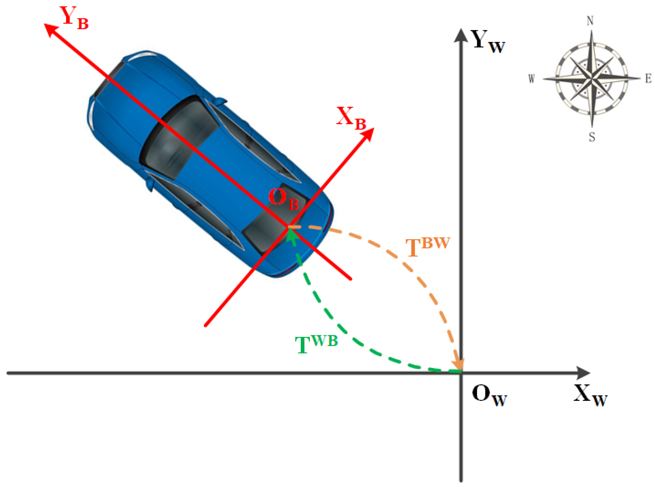
Figure 2 shows the coordinate system { W } and { B } in the 2D plane and the relationship between them. The body coordinate system { B } changes with the movement of the vehicle. T k WB represents the transformation between the coordinate system { W } and { B } at time t k , which can also denote the pose of the vehicle at time t k . On the contrary, T k BW transforms the coordinate system { B } to { W } and T k BW = T k WB 1 . Moreover, Δ T k 1 , k B , which could be obtained from the IMU, represents the relative transformation of the vehicle between time t k 1 and t k . The relationship between Δ T k 1 , k B and T k WB can be expressed as:
Δ T k 1 , k B = T k 1 WB 1 T k WB .
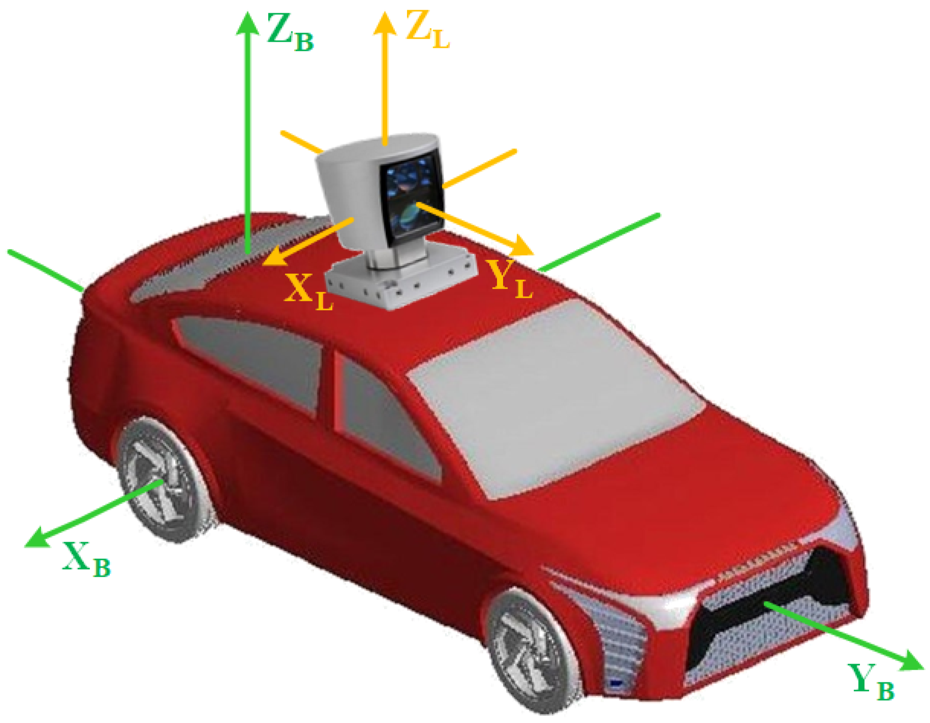
In addition, the relationship between the coordinate system { B } and { L } is shown in Figure 3.
We use T k WL to denote the pose of the lidar at time t k Δ T k 1 , k L represents the relative transformation of the lidar between time t k 1 and t k . The transformation T BL , which transforms the coordinate system { B } to { L } , can be obtained from the hand–eye calibration.
The transformation T can be expressed by:
T = R p 0 T 1 ,
where R R 3 × 3 represents the rotational matrix and p R 3 is the translational vector.
In Lie Group [19], T belongs to the Special Euclidean group SE ( 3 ) and the rotational matrix R belongs to the Special Orthogonal group SO ( 3 ) . Correspondingly, the se ( 3 ) and so ( 3 ) are two kinds of Lie Algebra. θ so ( 3 ) indicates the rotation angle which can be expressed as θ = θ n , where θ represents the magnitude of the rotation angle and n denotes the rotation axis. The pose can thus be represented by ξ = θ p T se ( 3 ) .
The exponential map and logarithmic map can be used to derive the relationship between the Lie Group and the Lie Algebra. For example, T can be represented by the exponential map of the ξ , namely, T = exp ξ . Conversely, ξ can be represented by the logarithmic map of the T , namely, ξ = log T .
The exponential map between θ and R can be formulated by using the Rodriguez formula:
R = cos θ · I + 1 cos θ · n · n T + sin θ · n .
The operator ∧ maps a vector to a skew-symmetric matrix as Equation (4), and the operator ∨ maps a skew symmetric matrix back to a vector.
θ = θ x θ y θ z = 0 θ z θ y θ z 0 θ x θ y θ x 0 .
The notation of the data used in our system are specified as follows. Each type of data used in our system is composed of the timestamp and the data itself. The timestamp is defined as the time when the data is generated. t B denotes the timestamp of the IMU measurement and t L represents the timestamp of the lidar point clouds. f k L indicates all points generated from the lidar during [ t k 1 L , t k L ] . In addition, the i-th point generated by the b-th laser beam is denoted as X ( i , b , k ) L in the lidar coordinate system { L } . The number of points received per laser beam is denoted as S b and i [ 1 , S b ] .

3.2. Motion Prior from IMU and Wheel Encoder

It is well-known that the accelerometer in the IMU is affected by the gravity, and it needs to be integrated twice to obtain the translational vector [20]. In contrast, the gyro in the IMU directly measures the angular velocity, and it only needs to be integrated once to obtain the rotation angle. It is reasonable to believe that the angular output from the IMU is much more accurate than the translational measurement.
For the ground vehicle, besides IMU, it is also equipped with the wheel encoder. The wheel encoder directly measures the rotation of the wheel, and thus provides a much more accurate translational measurement.
In this paper, we try to combine the angular output from the IMU and the translational output from the wheel encoder to obtain the motion prior.
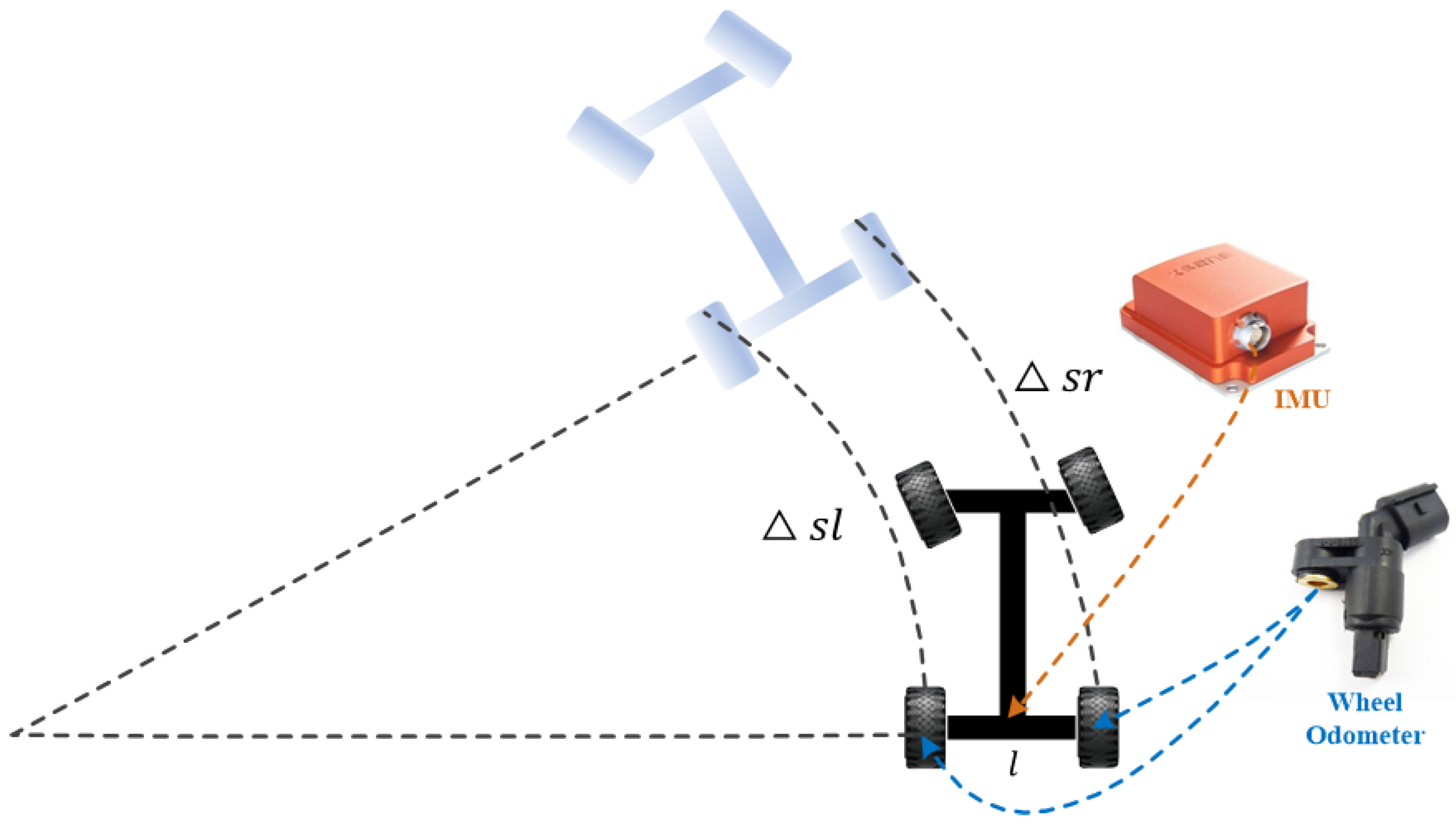
The motion model of the vehicle can be simplified as Figure 4. We mount the IMU at the center of two rear wheels, and mount two wheel encoders on the left and right rear wheels, respectively. The black car denotes the position of the vehicle at the previous moment t k 1 B , and the blue car indicates its position at the current time t k B . Δ s l and Δ s r represent the traveled distances of the left rear wheel and the right rear wheel during the short period of time.
Firstly, we compute the rotation matrix R k WB by triaxial angular velocities of the IMU. We introduce the following kinematic model [21]:
d R τ BW d t = R τ BW ω τ x ω τ y ω τ z .
In Equation (5), R τ BW indicates the rotation matrix from the coordinate system { B } to { W } . ω τ x , ω τ y , and ω τ z represent the instantaneous angular velocities of the IMU.
By assuming the angular velocity of the IMU constant during [ t k 1 B , t k B ] , we integrate Equation (5) from t k 1 B to t k B and solve the differential equation. The rotation matrix R k BW can be obtained by:
R k BW = R k 1 BW Exp ω k Δ t .
To compute the translational component p k WB of the pose T k WB , we approximate the traveled distance Δ s of the vehicle to be the average of the two rear wheels.  Δ s indicates the relative displacement of the vehicle during [ t k 1 B , t k B ] in the body coordinate system { B } and the instantaneous speed of the vehicle can be denoted as v = Δ s / ( t k B t k 1 B ) . We assume the velocity of the vehicle to be constant during [ t k 1 B , t k B ] , where the wheel encoder always records the distance traveled along the heading direction of the vehicle. Thus, the instantaneous velocity vector can be denoted as v k B = [ v 0 0 ] T . The relationship between the velocity vector v k W in the coordinate system { W } and the velocity vector v k B in the coordinate system { B } is:
v k W = R k WB v k B .
Using p k 1 WB , R k WB , and v k W , the translational component p k WB can be computed as:
p k WB = p k 1 WB + v k W t k t k 1 = p k 1 WB + R k WB Δ s 0 0 T .
Since both the IMU and the wheel encoder output data at a frequency of 100 Hz, we use two separate buffers to cache these two kinds of data. These two sources of information are then fused by Equations (6) and (8). This fusion process only involves a few operators, and usually takes less than 1 millisecond. Therefore, the fusion output, which we term as the motion prior data, is also generated at 100 Hz.

3.3. Pre-Processing Step 1: Lidar-IMU Hand–Eye Calibration

As described before, the lidar point clouds are represented in the lidar coordinate system { L } . Taking the lidar point clouds of two frames f k 1 L and f k L as inputs, we can calculate Δ T k 1 , k L by the lidar odometry algorithm. Δ T k 1 , k L indicates the relative transformation in the coordinate system { L } . However, the Δ T k 1 , k B obtained from the IMU is expressed in the body coordinate system { B } . Therefore, in order to utilize the IMU information, we need to establish the relationship between { L } and { B } first.
The calculation of the relative transformation T BL between { L } and { B } is a typical hand–eye calibration problem. Based on T BL , we can transform a point from the lidar coordinate system { L } to the body coordinate system { B } :
X ( i , b , k ) B = T BL X ( i , b , k ) L .
According to [22], we can formulate the hand–eye calibration problem between the coordinate system { L } and { B } as:
Δ T k , k 1 B T BL = T BL Δ T k , k 1 L .
Δ T k 1 , k B and Δ T k 1 , k L are inputs of Equation (10). Let the timestamps of frames f k L and f k 1 L be τ k L and τ k 1 L , respectively. We firstly find the nearest timestamps τ k B and τ k 1 B from the IMU, then T k WB and T k 1 WB can be obtained. The relative transformation Δ T k 1 , k B can be computed by Equation (1). We then use Δ T k 1 , k B as the initial guess and Δ T k 1 , k L can be obtained from the lidar odometry.
Equation (10) can be solved by calculating the rotational and translational component separately. The rotational component is:
Δ R k , k 1 B R BL = R BL Δ R k , k 1 L ,
and the translational component is:
Δ R k , k 1 B p BL + Δ p k , k 1 B = R BL Δ p k , k 1 L + p BL .
There are many methods to solve Equations (11) and (12). According to [23], the method proposed by Tsai et al. [24] exhibits the best performance. We therefore chose to use this method.
In our approach, multiple pairs of transformation Δ T i , i 1 L and Δ T i , i 1 B are needed. To reduce the error of hand–eye calibration [25,26], the following requirements need to be met:
  • To avoid the intra-frame distortion caused by the vehicle’s own movement, the frames should be chosen when the vehicle is stationary.
  • The relative rotation angle of the two frames needs to be greater than 90 degrees, and the relative translation distance should be small.
  • The rotational axes for these multiple transformation pairs should not be parallel.
After completing the hand–eye calibration, each point of the frame f k L can be transformed by Equation (9) and be represented in the coordinate system { B } .

3.4. Pre-Processing Step 2: Intra-Frame Correction

As mentioned in Section 3.1, it usually takes 100 ms for the lidar to spin a full circle. During this time, the vehicle also keeps moving. Some of these data are received at the previous moment t k L t j ( t j ( 0 , 100 ) ( ms ) ) and their coordinates are represented in the coordinate system corresponding to the moment t k L t j . These points can be denoted as X ( i , b , k j ) B . If we want to represent these points in the coordinate system corresponding to time t k L , we need to transform the point X ( i , b , k j ) B to X ( i , b , k ) B . This transformation is usually called “correction” or “rectification” of the lidar scan.
There are two common ways to rectify the distorted point clouds. One utilizes the information of IMU [16,27]. We make some improvements in this method which is described in Section 3.4.1. The other one uses the previous registration results [15], which is presented in Section 3.4.2. Furthermore, we also propose an interesting two-step correction procedure which does not rely on the IMU in Section 3.4.3.

3.4.1. Rectification with the Aid of IMU

In this method, we try to use IMU to rectify the raw points. Let the pose at time t k L and t k 1 L be T q WB and T p WB . Since the IMU data is generated at a frequency of 100 Hz and the lidar point clouds are generated at a frequency of 10 Hz, there are always nine frames of IMU data between the pose T p WB and T q WB . Therefore, ten relative transformations Δ T m 1 , m B ( m ( p , q ] ) can be obtained by Equation (1) and each Δ T m 1 , m B represents the relative transformation during [ t m 1 B , t m B ] , where t m B t m 1 B equals to 10 ms.
Since the rotational velocity of the lidar is constant during [ t k 1 L , t k L ] , the rotation angle of the lidar per 10 ms is also fixed. We can separate all points of a frame f k L into ten sets, and the ID of points in each set can be denoted as i [ m 1 p q p × S b , m p q p × S b ] . Let the total number of points in each set be S e , which is equal to S b / 10 . We further assume that the motion of the vehicle is constant during [ t m 1 B , t m B ] . Each set of points now correspond to a unique relative transformation Δ T m , m 1 B which can also be denoted as e x p Δ ξ m 1 , m .
We linearly interpolated e x p Δ ξ m 1 , m to transform point X ( i , b , k j ) B to X ( i , b , m 1 ) B . Then, X ( i , b , m 1 ) B will be transformed to X ( i , b , k ) B by Δ T q , m 1 B . The whole rectification process can be denoted as:
X ^ ( i , b , k ) B = Δ T q , m 1 B · exp Δ ξ m 1 , m · i % S e S e · X ( i , b , k j ) B ,
where A % B is used to compute the remainder when A is divided by B, and X ^ ( i , b , k ) B represents the undistorted point after rectification.

3.4.2. Rectification by Previous Registration Results

This approach assumes that the motion of the vehicle is constant during t k 2 L , t k L . Thus, it can assume that the relative transformation Δ T k 1 , k 2 B between frame f k 1 L and f k 2 L is the same as the relative transformation Δ T k , k 1 B between frame f k L and f k 1 L . Therefore, we can linearly interpolate the relative transformation e x p Δ ξ k 1 , k 2 to rectify the raw distorted points in frame f k L as:
X ^ ( i , b , k ) B = exp Δ ξ k 1 , k 2 · i S b · X ( i , b , k j ) B .

3.4.3. Rectification by Registering Two Distorted Point Clouds

In this approach, we note that intra-frame correction is in fact quite related to inter-frame registration. As the task of intra-frame correction is to estimate the lidar motion between 0 ms and 100 ms, inter-frame registration tries to estimate the motion between 100 ms and 200 ms. Both frame a (corresponding to the lidar date generated between 0 ms and 100 ms) and frame b (generated between 100 ms and 200 ms) are distorted point clouds. It is reasonable to assume that the degree of distortion of these two frames are quite similar. We could thus directly register these two frames without any intra-frame correction first, and then use the registration result to correct each frame.
Let the relative transformation obtained from registering two distorted point clouds be Δ T ˜ k , k 1 B . We assumed that Δ T ˜ k , k 1 B can approximate the lidar motion between time t k L , t k 1 L and linearly interpolate e x p Δ ξ ˜ k , k 1 to rectify the raw distorted points of f k L , as in Equation (15).
X ^ ( i , b , k ) B = exp Δ ξ ˜ k , k 1 · i S b · X ( i , b , k j ) B .
The undistorted frame after rectification is denoted as f ^ k L . In Section 4, we do experiments to compare these three approaches.

3.5. Intermediate Step: Inter-Frame Registration

To register two frames of point clouds, we could use any off-the-shelf scan registration approaches, such as ICP, NDT, and LOAM. To successfully apply these approaches, it always requires an accurate initial guess for the estimated transformation. Just as mentioned previously, the problem of inter-frame registration is, in fact, quite related to intra-frame correction. Therefore, the approaches mentioned in Section 3.4 can also be applied here. We can either use the registration result of the previous two frames, or use the IMU data directly. We undertake experiments to compare these two approaches, presented in Section 4.

3.6. Output Step: Fusion in an EKF Framework

3.6.1. Basic Concepts

The Extended Kalman filter (EKF) [28] is one of the most commonly used data fusion algorithms. It is a recursive state estimator for the nonlinear system, and the state is assumed to satisfy a Gaussian distribution. A typical EKF algorithm consists of two steps: a prediction step, and an update step.
In the prediction step, the previous state x k 1 is used to compute a priori estimate of the current state by:
x ¯ k = f x ^ k 1 , P ¯ k = F P ^ k 1 F T + R ,
where R is the covariance of the process noise. x ¯ k and P ¯ k are the mean and covariance matrices of the prior distribution of the state x k , respectively. x ^ k 1 and P ^ k 1 are the mean and covariance matrices of the posterior Gaussian distribution of the state x k 1 . By performing a first-order Taylor expansion to the function f at the mean of the state x k 1 , the first-order partial derivative can be denoted as the Jacobian matrix F :
F = f x k 1 | x ^ k 1 .
In the update step, the priori estimate of the current state is combined with the current observation z k to refine the state estimate and obtain the posteriori state estimate x k , which can be formulated as:
K k = P ¯ k H T H P ¯ k H T + Q 1 , x ^ k = x ¯ k + K k z k h x ¯ k , P ^ k = I K k H P ¯ k ,
where Q represents the covariance of the measurement noise. K k is the Kalman gain and the posteriori state estimation x k N x ^ k , P ^ k . Similarly, a first-order Taylor expansion to the function h can be performed at the mean of the prior distribution of the state x k . The first-order partial derivative could be defined as the Jacobian matrix H :
H = h x k | x ¯ k .
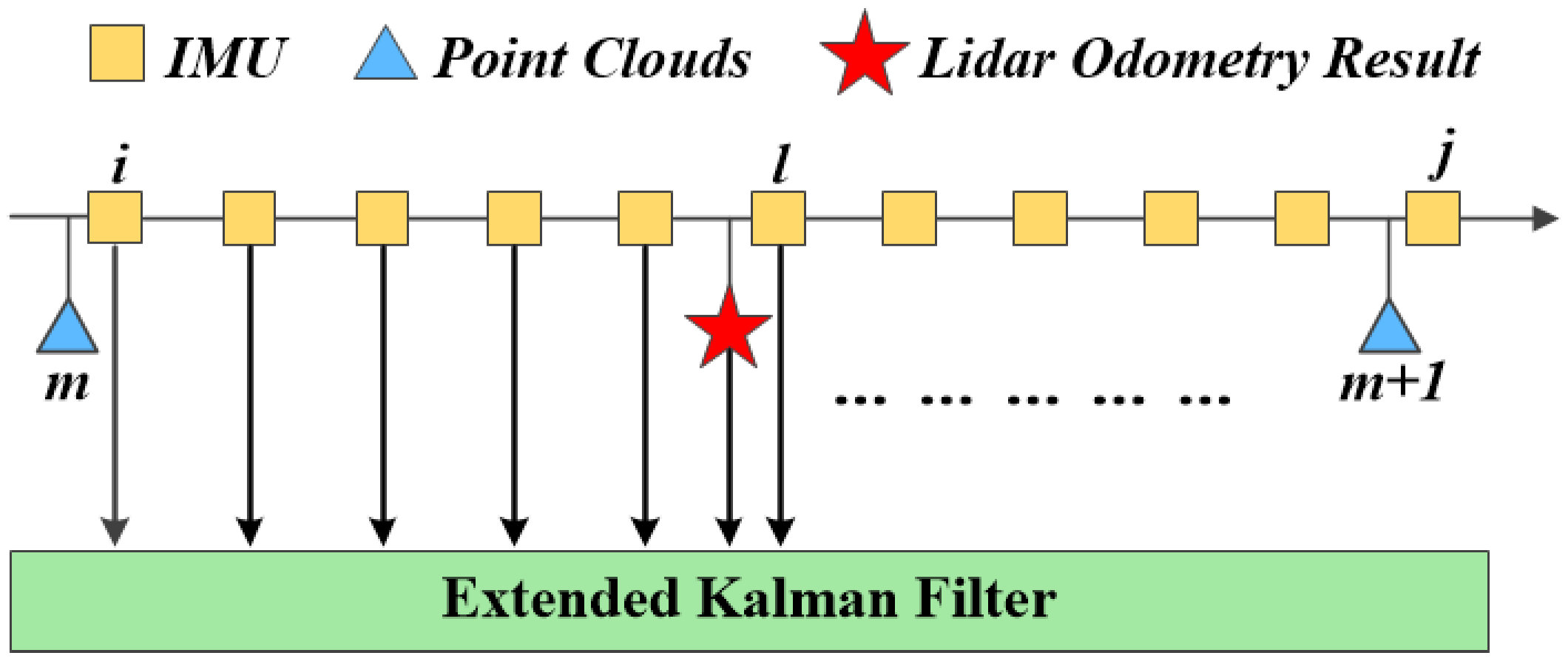
In this section, We use an EKF framework to fuse the IMU and the results obtained from the lidar odometry, as shown in Figure 5. Let the motion prior model presented in Section 3.2 be the system model and the results from the lidar odometry (which is denoted as the red star in Figure 5) be the measurements. The system model and measurement model are described as follows.

3.6.2. System Model

Since the main purpose of our system is to obtain the pose of the vehicle, we could use the Lie Algebra ξ to define the state vector x k at time t k as:
x k = θ k p k T se ( 3 ) .
By utilizing the logarithmic map and the approximate Baker-Campbell-Hausdorff (BCH) formula [21], the R k WB obtained from the Equation (6) can be converted to:
θ k = J l 1 θ k 1 · ω k Δ t + θ k 1 ,
where J l 1 θ k denotes the right BCH Jacobian of SO ( 3 ) and it equals to:
J l 1 θ k = θ k 2 cot θ k 2 I + 1 θ k 2 cot θ k 2 n k n k T θ k 2 n k ,
and J l 1 θ k can be denoted as:
J l 1 θ k = J 1 1 θ k J 2 1 θ k J 3 1 θ k J 4 1 θ k J 5 1 θ k J 6 1 θ k J 7 1 θ k J 8 1 θ k J 9 1 θ k .
Combining the Equations (8), (21) and (23), the state transition equation could be defined as:
x k = x k 1 + J l 1 θ k 1 · ω k Δ t R k WB ( 1 : 3 , 1 ) · Δ s ,
where R k WB is computed by θ k x , θ k y and θ k z according to Equation (3) and R k WB ( 1 : 3 , 1 ) means the first column of the R k WB .
According to Equations (17) and (24), F can be derived as:
F = F θ θ 0 3 × 3 F p θ I 3 × 3 R 6 × 6 ,
where F θ θ R 3 × 3 , and it can be computed by:    
F θ θ = I 3 × 3 + J l 1 θ k 1 θ k 1 x · ω k Δ t T J l 1 θ k 1 θ k 1 y · ω k Δ t T J l 1 θ k 1 θ k 1 z · ω k Δ t T T .
F p θ can be computed by:
F p θ = R k WB ( 1 : 3 , 1 ) θ k 1 x R k WB ( 1 : 3 , 1 ) θ k 1 y R k WB ( 1 : 3 , 1 ) θ k 1 z .
The prior probability distribution of the state x k could then be obtained by the Equation (16).

3.6.3. Measurement Model

The measurement vector z k is denoted as:
z k = θ z k x θ z k y θ z k z p z k x p z k z p z k z T .
According to Figure 5, the lidar odometry algorithm starts to run at time t m L , but the result is obtained at time t k , which is several tens of milliseconds after t m L . We assume that the pose of the vehicle at time t m L and t k were approximately equal to T i WB and T l WB . Both T i WB and T l WB can be obtained from the IMU data.
The relationship between the measurement z k and the real state x k of the vehicle at time t k can be indicated by Δ T i , l B , which can also be denoted as Δ ξ i , l = Δ θ i , l Δ p i , l T . The observation equation could then be represented as:
z k = θ k Δ p i , l + J l 1 θ k · Δ θ i , l Δ R i , l B · p k .
According to Equations (19) and (29), H can be derived as:
H = H θ θ 0 3 × 3 0 3 × 3 H p p ,
where H p p = Δ R i , l WB R 3 × 3 , H θ θ R 3 × 3 and H θ θ can be computed by:
H θ θ = J l 1 θ k θ k x · Δ θ i , l T J l 1 θ k θ k y · Δ θ i , l T J l 1 θ k θ k z · Δ θ i , l T T .
Based on the covariance matrix P ¯ k from Equation (16) and the Jacobian matrix H from Equation (30), the Kalman gain K k and the posteriori state estimation could be computed by the Equation (18).
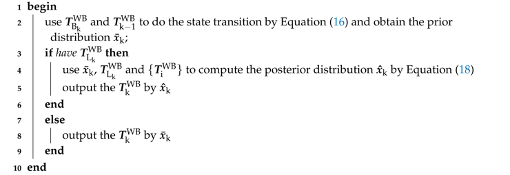
This fusion framework is summarized in Algorithm 1.
Algorithm 1: The fusion framework of our system.
    input: The history pose set { T i WB } and pose T B k WB at time t k B from the IMU; pose T L k WB at time t k L from the lidar odometry; previous pose T k 1 WB
    output: Current pose T k WB
Applsci 09 01506 i001

4. Experimental Results

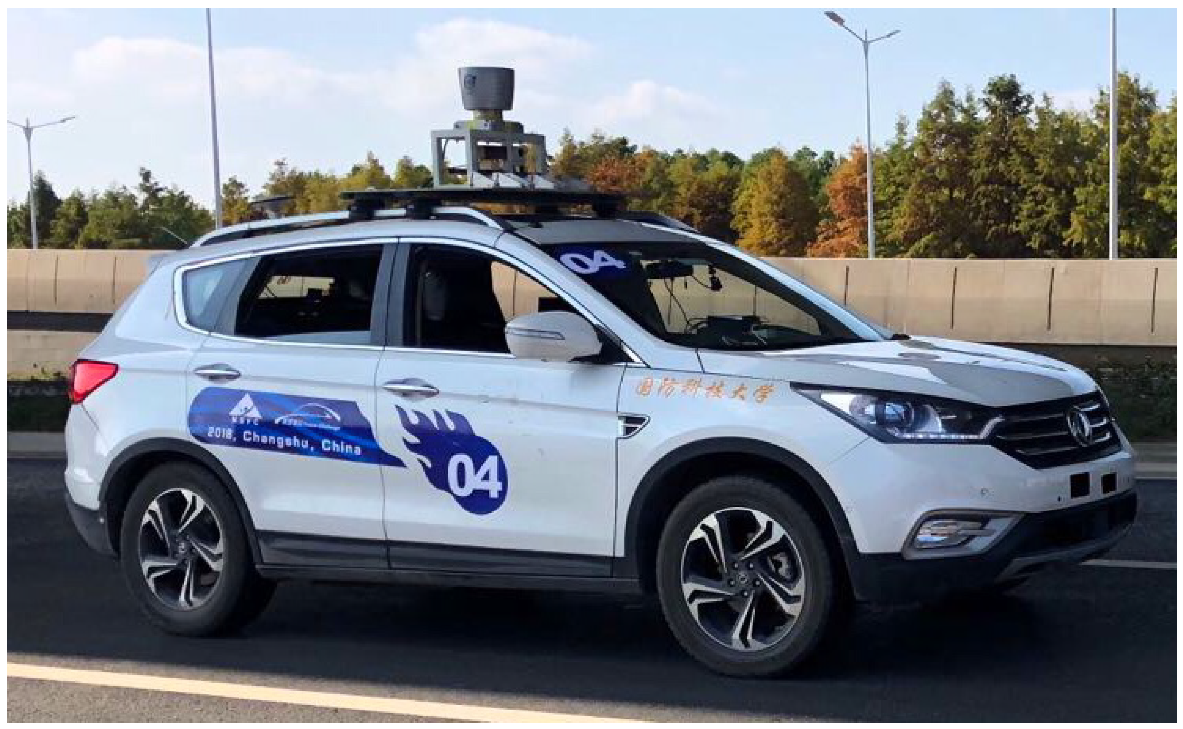
The platform used in the following experiments is shown in Figure 6. The vehicle is equipped with a Velodyne HDL-64E lidar, a Xsens MTI300 IMU, two photoelectric encoders, a NovAtel SPAN-CPT GNSS/INS system, and a Nova 5100 industrial computer. The lidar is mounted on the top of the car, and it has 64 beams which could generate over 1.3 million points per second with a high range accuracy. The horizontal Field of View (FOV) is 360 , the vertical FOV is 26 . 8 , and the maximal detection distance is 120 m. The NovAtel GNSS/INS system provides localization results with centimeter-level accuracy, which can be served as the ground truth.

4.1. Experiments on Hand–Eye Calibration

As described in Section 3.3, in order to perform the lidar-IMU hand–eye calibration, we need to utilize multiple pairs of relative transformations { Δ T k 1 , k B , Δ T k 1 , k L } .
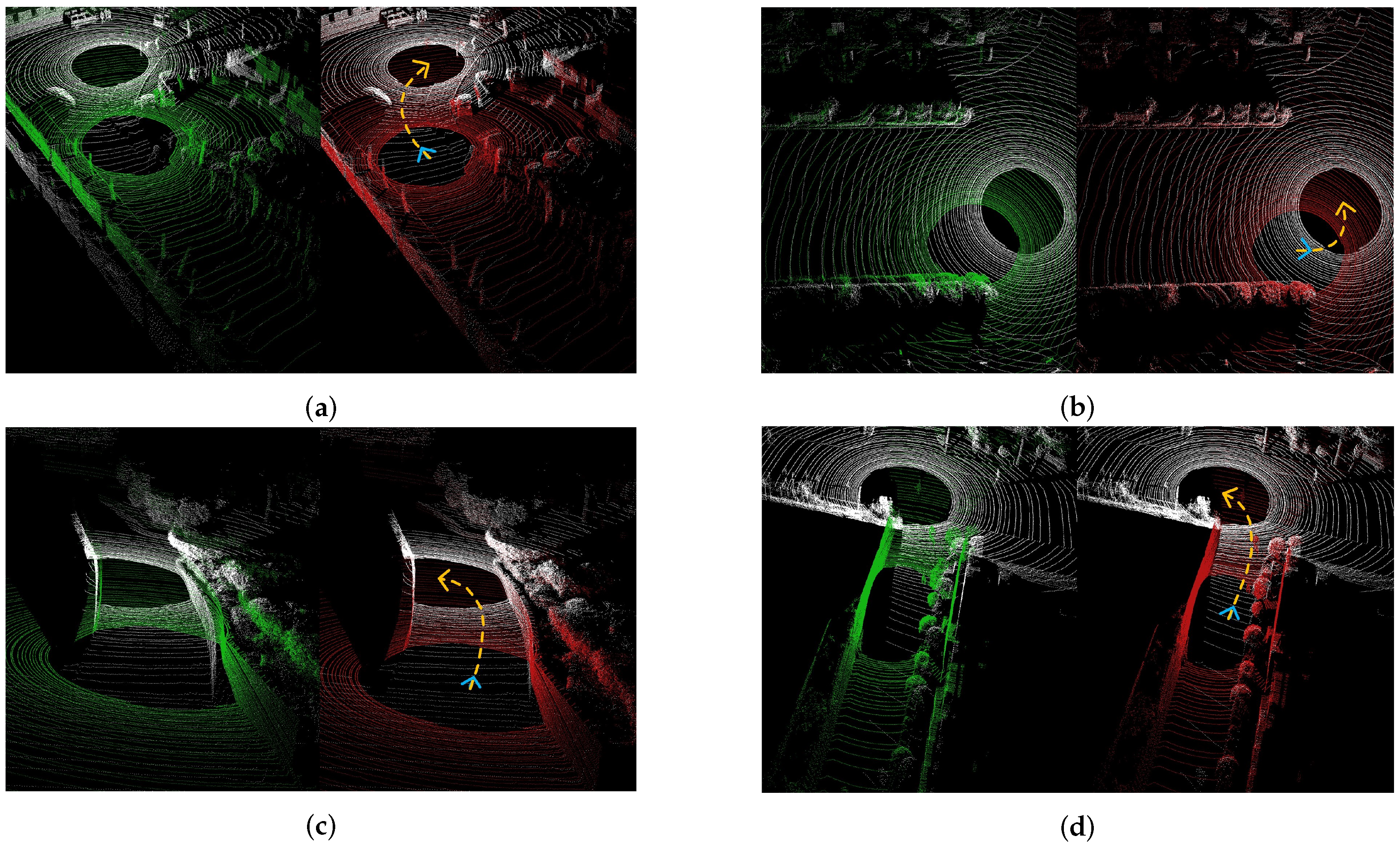
We choose the frame pairs { f i L , f i 1 L } before and after the vehicle makes a turn. In addition, all the frames are collected when the vehicle is stationary. Figure 7 shows several transformation pairs we have chosen. In each sub-figure, the left part is the registration result before the hand–eye calibration, whilst the right half is the result after hand–eye calibration. It can be seen that f i L and f i 1 L are much better-registered in the right half of Figure 7a–d than the left half, which indicates the importance of hand–eye calibration.
Since the ground truth of T BL is impossible to be obtained, we could not verify the calibration result directly. However, we could use the IMU data to assemble different frames together, and the quality of the assembled scene can be used to evaluate the accuracy of the hand–eye calibration result. Figure 8 shows the assembled scene when the vehicle makes a turn at the intersection. Figure 8a is the assembled result before hand–eye calibration, which is very vague, while the result after the hand–eye calibration in Figure 8b is much clearer. This suggests that the result of our hand–eye calibration is accurate.
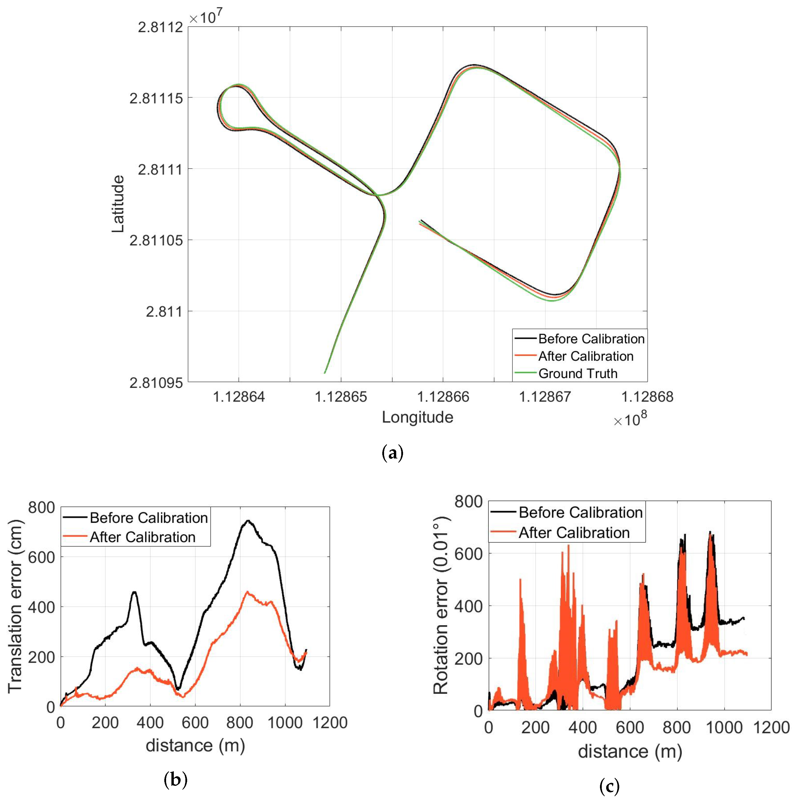
To quantitatively test the effect of hand–eye calibration, we choose the LOAM algorithm as the lidar odometry algorithm, and compare the estimated trajectories with the ground-truth trajectory generated by the GNSS/INS system. Figure 9 illustrates the localization result before and after hand–eye calibration. The translation error and rotation error are shown in Figure 9b,c, where the horizontal axis represents the traveled distance and the vertical axis shows the errors. It is obvious that the translation error and the rotation error are significantly reduced after the hand–eye calibration.

4.2. Experiments on Intra-Frame Correction

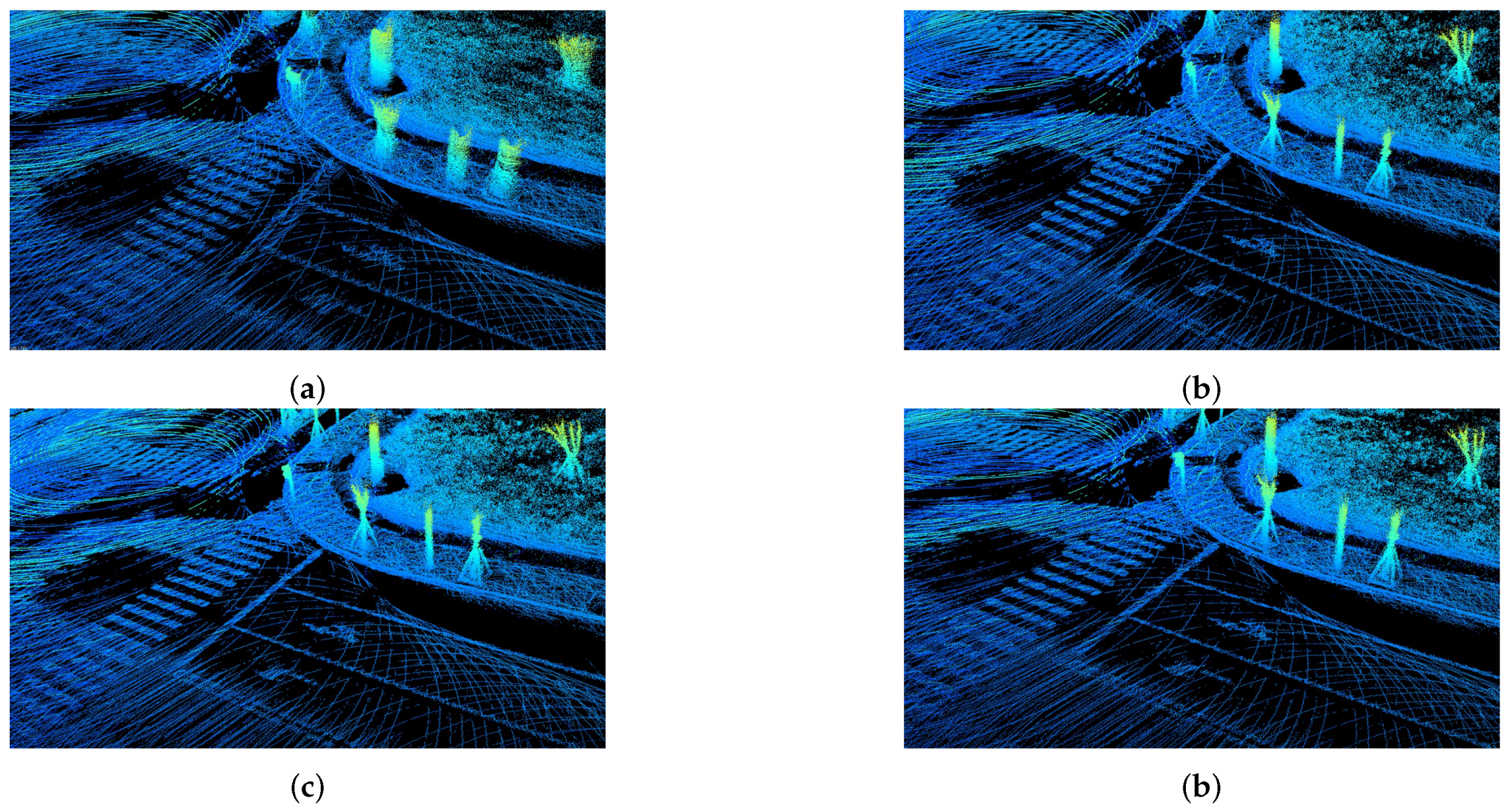
Based on the hand–eye calibration results, we could also use the 3D reconstruction results to qualitatively test the three rectification methods introduced in Section 3.4. In order to test the result of the rectification, the vehicle should run fast to amplify the intra-frame distortion. Therefore, we carry out this experiment when the vehicle drives at around 60 km/h, and the results are shown in Figure 10.
Figure 10a–d represent different 3D reconstruction results when the vehicle is making a turn. Figure 10a is the result without any rectification, and the reconstructed scene is quite blurry. Figure 10b–d show the results when the distorted point clouds are rectified by the previous registration result, by registering two distorted point clouds and by the IMU data. The results obtained by these three approaches are all much better than the one without rectification. Moreover, the average processing time for these three methods applied on 2000 frames of point clouds is displayed in Table 1. It is seen that the approach of registering two distorted point clouds is the most computational expensive approach.
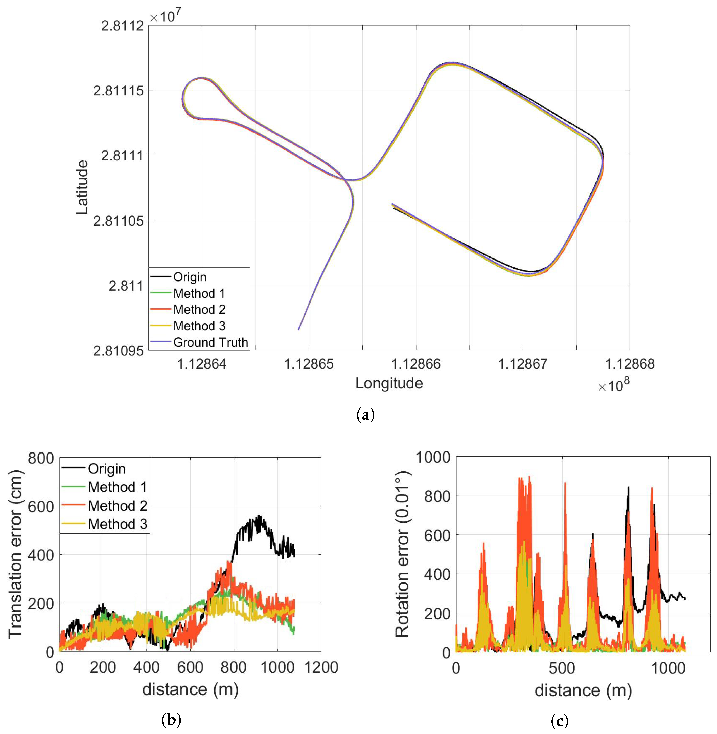
To quantitatively test the effect of intra-frame correction, LOAM is also used as the lidar odometry algorithm, and the localization accuracy is compared with the ground-truth trajectory. Figure 11 compares the localization results with/without rectification. The trajectories generated by the three rectification methods and without rectification are compared with the ground truth in Figure 11a, where “Method 1” represents rectification by previous registration, “Method 2” is the approach of registering two distorted point clouds, and “Method 3” indicates rectification by IMU data. In addition, Figure 11b,c compare the translation error and rotation error of these approaches.
It can be seen that both the translation error and the rotation error are significantly reduced after rectification, and “Method 3” exhibits the best performance, followed by “Method 1” and “Method 2”. A detailed error comparison is presented in Table 2.

4.3. Experiments on Inter-Frame Registration

4.3.1. Tests with Different Methods of Assigning Initial Guess

In this experiment, two methods of assigning initial guess for the lidar odometry algorithm are compared—namely, using the IMU data or the registration result from the previous two scans. In both approaches, the raw distorted point clouds are rectified by the IMU data, and LOAM is used as the lidar odometry algorithm.
The tests are conducted when the vehicle drives at different speeds: a relatively slow speed of around 25 km/h, and a faster speed of around 60 km/h. A detailed error comparison is shown in Table 3. It can be seen that using the IMU data as the initial guess always produces a better result than using the registration result from the previous two scans, especially when the vehicle drives at a faster speed.

4.3.2. Tests with Different Lidar Odometry Algorithms

Here, we compare three popular lidar odometry algorithms: ICP, NDT, and LOAM. During the experiments, the point clouds are rectified by the IMU data. The vehicle drives at a speed around 25 km/h, and the overall distance is about 1.1 km. A detailed error comparison is shown in Table 4. It is obvious that LOAM performs much better than NDT and ICP.

4.3.3. Tests in Both Urban and Off-Road Environments

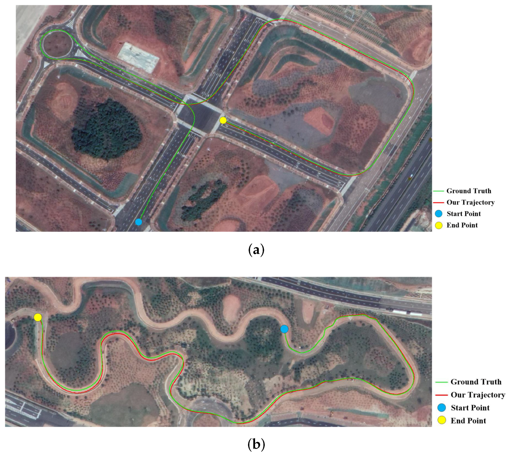
Our algorithm is tested in both urban and off-road environment. We choose to use LOAM as the lidar odometry algorithm. The point clouds are rectified by the IMU data. In the urban environment, the vehicle drives at a speed of around 25 km/h, and the overall distance is about 1.1 km. In the off-road environment, the vehicle drives at a speed of around 15 km/h and the overall distance is about 1.0 km. The trajectories generated by our method are compared with the ground truth in Figure 12. A detailed error comparison is shown in Table 5. It is seen that our approach is applicable for both the urban and off-road environments, whilst the error in the off-road scenario is slightly higher than the urban environment.

4.4. Experiments in GNSS-Denied Environment

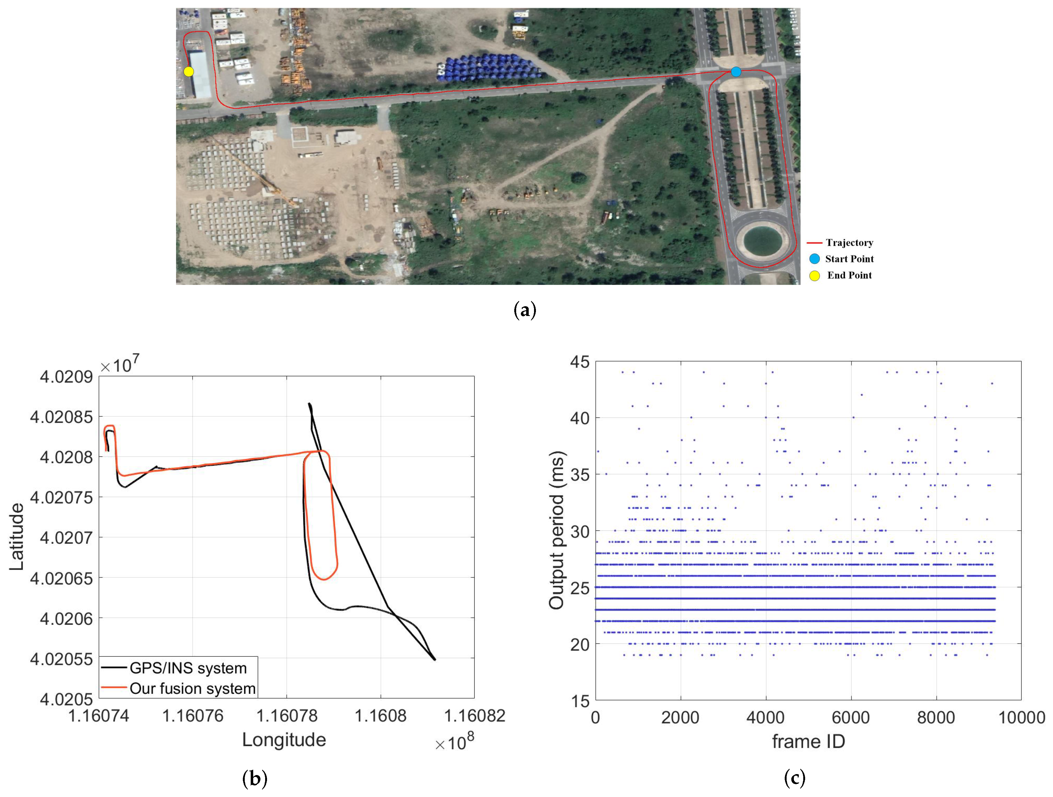
Finally, we test our whole localization system in the GNSS-Denied environment. Figure 13a shows the trajectory generated by our localization system when the UGV drives at a speed of 20 km/h. By projecting the trajectory to the satellite image, we find that the position drift is quite small. Figure 13b compares the trajectories generated by our localization system and by the disturbed GNSS/INS system. Figure 13c shows the output frequency of our localization system. The average output frequency is around 39.7 Hz. In summary, no matter whether the GNSS signal is available or not, our system can output precise and high-frequency localization results.

5. Conclusions

In this paper, we present a novel approach for combining the IMU data with lidar odometry. The proposed localization system could generate stable, accurate, and high-frequency localization results. Since our system does not recognize the loop closure, we can further extend our work to enable the ability of loop-closure detection.

Author Contributions

Conceptualization, H.F.; Data curation, H.X.; Formal analysis, H.X.; Funding acquisition, B.D.; Investigation, H.X.; Methodology, H.F. and H.X.; Project administration, B.D.; Resources, H.F. and B.D.; Software, H.F. and H.X.; Supervision, B.D.; Validation, H.F.; Original draft, H.X.; Review and editing, H.F.

Funding

This work was supported by the National Natural Science Foundation of China under No. 61790565.

Conflicts of Interest

The authors declare no conflict of interest.

References

  1. Kos, T.; Markezic, I.; Pokrajcic, J. Effects of multipath reception on GPS positioning performance. In Proceedings of the Elmar-2010, Zadar, Croatia, 15–17 September 2010; pp. 399–402. [Google Scholar]
  2. Kohlbrecher, S.; von Stryk, O.; Meyer, J.; Klingauf, U. A flexible and scalable SLAM system with full 3D motion estimation. In Proceedings of the 2011 IEEE International Symposium on Safety, Security, and Rescue Robotics, Kyoto, Japan, 1–5 November 2011; pp. 155–160. [Google Scholar]
  3. Gao, Y.; Liu, S.; Atia, M.M.; Noureldin, A. INS/GPS/LiDAR integrated navigation system for urban and indoor environments using hybrid scan matching algorithm. Sensors 2015, 15, 23286–23302. [Google Scholar] [CrossRef] [PubMed]
  4. Tang, J.; Chen, Y.; Niu, X.; Wang, L.; Chen, L.; Liu, J.; Shi, C.; Hyyppä, J. LiDAR scan matching aided inertial navigation system in GNSS-denied environments. Sensors 2015, 15, 16710–16728. [Google Scholar] [CrossRef] [PubMed]
  5. Liu, S.; Atia, M.M.; Gao, Y.; Givigi, S.; Noureldin, A. An inertial-aided LiDAR scan matching algorithm for multisensor land-based navigation. In Proceedings of the 27th International Technical Meeting of the Satellite Division of the Institute of Navigation, Tampa, FL, USA, 8–12 September 2014; pp. 2089–2096. [Google Scholar]
  6. Ye, H.; Liu, M. LiDAR and Inertial Fusion for Pose Estimation by Non-linear Optimization. arXiv, 2017; arXiv:1710.07104. [Google Scholar]
  7. Pierzchala, M.; Giguere, P.; Astrup, R. Mapping forests using an unmanned ground vehicle with 3D LiDAR and graph-SLAM. Comput. Electron. Agric. 2018, 145, 217–225. [Google Scholar] [CrossRef]
  8. Besl, P.J.; McKay, N.D. A Method for Registration of 3-D Shapes. IEEE Trans. Pattern Anal. Mach. Intell. 1992, 14, 239–256. [Google Scholar] [CrossRef]
  9. Pomerleau, F.; Colas, F.; Siegwart, R.; Magnenat, S. Comparing ICP variants on real-world data sets. Auton. Robots 2013, 34, 133–148. [Google Scholar] [CrossRef]
  10. Stoyanov, T.; Magnusson, M.; Andreasson, H.; Lilienthal, A.J. Fast and accurate scan registration through minimization of the distance between compact 3D NDT representations. Int. J. Robot. Res. 2012, 31, 1377–1393. [Google Scholar] [CrossRef]
  11. Magnusson, M.; Lilienthal, A.; Duckett, T. Scan registration for autonomous mining vehicles using 3D-NDT. J. Field Robot. 2007, 24, 803–827. [Google Scholar] [CrossRef] [Green Version]
  12. Nguyen, V.; Gachter, S.; Martinelli, A.; Tomatis, N.; Siegwart, R. A comparison of line extraction algorithms using 2D range data for indoor mobile robotics. Auton. Robots 2007, 23, 97–111. [Google Scholar] [CrossRef]
  13. Aghamohammadi, A.; Taghirad, H. Feature-Based Laser Scan Matching for Accurate and High Speed Mobile Robot Localization. In Proceedings of the EMCR, Freiburg, Germany, 19–21 September 2007. [Google Scholar]
  14. Furukawa, T.; Dantanarayana, L.; Ziglar, J.; Ranasinghe, R.; Dissanayake, G. Fast global scan matching for high-speed vehicle navigation. In Proceedings of the 2015 IEEE International Conference on Multisensor Fusion and Integration for Intelligent Systems (MFI), San Diego, CA, USA, 14–16 September 2015; pp. 37–42. [Google Scholar]
  15. Zhang, J.; Singh, S. LOAM: Lidar Odometry and Mapping in Real-time. In Proceedings of the Robotics: Science and Systems, Berkeley, CA, USA, 12–16 July 2014; pp. 109–111. [Google Scholar]
  16. Zhang, J.; Singh, S. Low-drift and real-time lidar odometry and mapping. Auton. Robots 2017, 41, 401–416. [Google Scholar] [CrossRef]
  17. Hemann, G.; Singh, S.; Kaess, M. Long-range GPS-denied aerial inertial navigation with LIDAR localization. In Proceedings of the 2016 IEEE/RSJ International Conference on Intelligent Robots and Systems (IROS), Daejeon, Korea, 9–14 October 2016; pp. 1659–1666. [Google Scholar]
  18. Wan, G.; Yang, X.; Cai, R.; Li, H.; Zhou, Y.; Wang, H.; Song, S. Robust and Precise Vehicle Localization Based on Multi-Sensor Fusion in Diverse City Scenes. In Proceedings of the 2018 IEEE International Conference on Robotics and Automation (ICRA), Brisbane, QLD, Australia, 21–25 May 2018; pp. 4670–4677. [Google Scholar]
  19. Barfoot, T.D. State Estimation for Robotics; Cambridge University Press: Cambridge, UK, 2017; pp. 231–234. [Google Scholar]
  20. Kepper, J.H.; Claus, B.C.; Kinsey, J.C. A Navigation Solution Using a MEMS IMU, Model-Based Dead-Reckoning, and One-Way-Travel-Time Acoustic Range Measurements for Autonomous Underwater Vehicles. IEEE J. Ocean. Eng. 2018, 1–19. [Google Scholar] [CrossRef]
  21. Forster, C.; Carlone, L.; Dellaert, F.; Scaramuzza, D. On-Manifold Preintegration for Real-Time Visual–Inertial Odometry. IEEE Trans. Robot. 2017, 33, 1–21. [Google Scholar] [CrossRef]
  22. Wu, L.; Ren, H. Finding the Kinematic Base Frame of a Robot by Hand-Eye Calibration Using 3D Position Data. IEEE Trans. Autom. Sci. Eng. 2017, 14, 314–324. [Google Scholar] [CrossRef]
  23. Shah, M.; Eastman, R.D.; Hong, T. An overview of robot-sensor calibration methods for evaluation of perception systems. In Proceedings of the Workshop on Performance Metrics for Intelligent Systems, College Park, MD, USA, 20–22 March 2012; pp. 15–20. [Google Scholar]
  24. Tsai, R.Y.; Lenz, R.K. A new technique for fully autonomous and efficient 3D robotics hand/eye calibration. IEEE Trans. Robot. Autom. 1989, 5, 345–358. [Google Scholar] [CrossRef]
  25. Dornaika, F.; Horaud, R. Simultaneous robot-world and hand-eye calibration. IEEE Trans. Robot. Autom. 1998, 14, 617–622. [Google Scholar] [CrossRef] [Green Version]
  26. Huang, K.; Stachniss, C. On Geometric Models and Their Accuracy for Extrinsic Sensor Calibration. In Proceedings of the 2018 IEEE International Conference on Robotics and Automation, Brisbane, QLD, Australia, 21–25 May 2018; pp. 1–9. [Google Scholar]
  27. Scherer, S.; Rehder, J.; Achar, S.; Cover, H.; Chambers, A.; Nuske, S.; Singh, S. River mapping from a flying robot: State estimation, river detection, and obstacle mapping. Auton. Robots 2012, 31, 189–214. [Google Scholar] [CrossRef]
  28. Cadena, C.; Carlone, L.; Carrillo, H.; Latif, Y.; Scaramuzza, D.; Neira, J.; Reid, I.; Leonard, J.J. Past, Present, and Future of Simultaneous Localization and Mapping: Toward the Robust-Perception Age. IEEE Trans. Robot. 2016, 32, 1309–1332. [Google Scholar] [CrossRef] [Green Version]
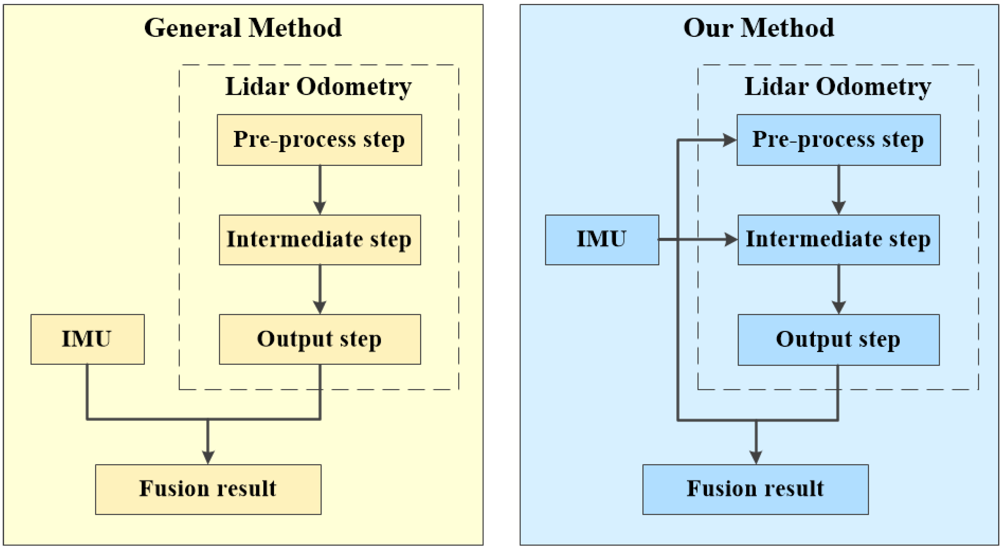
Figure 1. A typical lidar odometry algorithm can be roughly divided into three steps: a pre-processing step, an intermediate step, and an output step. Most existing lidar/Inertial Measurement Unit (IMU) fusion approaches try to fuse lidar odometry and the IMU in the output level [2,3,4,5,6,7]. In this paper, we try to utilize the IMU information in all the three steps.
Applsci 09 01506 g001
Figure 2. The relative relationship between the world coordinate system { W } and the body coordinate system { B } in the 2D plane, where the black axis indicates { W } and the red axis indicates { B } .
Applsci 09 01506 g002
Figure 3. The relationship between the body coordinate system { L } and the lidar coordinate system { B } , where the yellow axis indicates { L } and the green axis indicates { B } .
Applsci 09 01506 g003
Figure 4. Schematic diagram of the simplified vehicle motion model. The black car represents the previous position of the vehicle, and the blue car indicates its current position. During a time period, the left rear wheel travels a distance of Δ s l , and the right rear wheel travels Δ s r .
Applsci 09 01506 g004
Figure 5. The diagram of the proposed fusion framework. The yellow rectangle represents the IMU data, and the blue triangle indicates the lidar point clouds. The red star denotes the localization result output from the lidar odometry.
Applsci 09 01506 g005
Figure 6. Our experimental platform. It is equipped with a Velodyne HDL-64E Lidar, a Xsens MTI300 IMU, two photoelectric encoders, a NovAtel SPAN-CPT GNSS/INS system, and a Nova 5100 industrial computer.
Applsci 09 01506 g006
Figure 7. Four typical lidar pairs chosen to perform the hand–eye calibration. In each sub-figure, the left part is the registration result before the hand–eye calibration, whilst the right half is the result after hand–eye calibration. The yellow dotted line indicates the movement trajectory of the vehicle, while the yellow arrow and the blue arrow denote the orientation of the vehicle.
Applsci 09 01506 g007
Figure 8. The 3D reconstruction result when the vehicle turns around at the intersection. The left (a) is the result before hand–eye calibration, and the right (b) is the result after hand–eye calibration.
Applsci 09 01506 g008
Figure 9. The localization results before and after hand–eye calibration, where (a) compares the trajectories before/after hand–eye calibration with the ground truth; (b) compares the translation error before/after calibration, and rotation error is shown in (c). In this experiment, the UGV drives at a speed around 25 km/h, and the overall distance is about 1.1 km.
Applsci 09 01506 g009
Figure 10. The 3D reconstruction results to test the three rectification methods. (a) represents the result without any rectification, and (bd) show the results when the distorted point clouds are rectified by the previous registration result, by registering two distorted point clouds and by the IMU data, respectively.
Applsci 09 01506 g010
Figure 11. The localization results with/without rectification, where (a) compares the trajectories generated by the three rectification methods (Methods 1–3 represent rectification by the previous registration result, by registering two distorted point clouds and by the IMU data, respectively), the trajectory generated without rectification (Origin) and the ground truth; and (b,c) compare the translation error and rotation error among them, respectively. In this experiment, the UGV drives at a speed of around 60 km/h.
Applsci 09 01506 g011
Figure 12. The results in the urban environment and off-road environment. (a) shows the trajectory generated in the urban environment when the UGV drives at a speed of around 25 km/h, and (b) shows the trajectory generated in the off-road environment when the UGV drives at a speed of around 15 km/h.
Applsci 09 01506 g012
Figure 13. The results in a GNSS-deniedenvironment. (a) shows the trajectory generated by our system when the UGV drives at a speed around 20 km/h and the overall distance is about 1.3 km. (b) compares the trajectories generated by our system and by the disturbed GNSS/INS system. (c) shows the output period of our localization system during the whole process, and the average output frequency is about 39.7 Hz.
Applsci 09 01506 g013
Table 1. Computational efficiency of three rectification methods.
Rectification MethodsAverage Processing Time (ms)
By previous registration2.565
By registering two distorted point clouds68.504
By IMU data4.546
Table 2. Error comparison of three rectification methods.
Rectification MethodsMean Relative Position Error
Method 10.79%
Method 20.94%
Method 30.57%
Without Rectification2.28%
Table 3. Error comparison of different methods at the intermediate step.
Speed (km/h)Methods of Assigning Initial GuessMean Relative Position Error
25IMU0.31%
 Previous regist0.46%
60IMU0.57%
 Previous regist1.32%
Table 4. Error comparison of three lidar odometry algorithms.
Lidar Odometry MethodsMean Relative Position Error
ICP6.28%
NDT3.85%
LOAM0.31%
Table 5. Error comparison of diverse environments.
EnvironmentDistance (km)Mean Relative Position Error
Urban1.0970.31%
Off-road0.9830.93%