Review

Superfluids, Fluctuations and Disorder

by
Alberto Cappellaro
1,*,† and
Luca Salasnich
1,2,†
1
Dipartimento di Fisica e Astronomia ‘Galileo Galilei’ and CNISM, Università di Padova, Via Marzolo 8, I-35131 Padova, Italy
2
Istituto Nazionale di Ottica (INO) del Consiglio Nazionale delle Ricerche (CNR), Via Nello Carrara 1, I-50019 Sesto Fiorentino, Italy
*
Author to whom correspondence should be addressed.
These authors contributed equally to this work.
Appl. Sci. 2019, 9(7), 1498; https://doi.org/10.3390/app9071498
Submission received: 1 March 2019 / Revised: 8 April 2019 / Accepted: 8 April 2019 / Published: 10 April 2019
(This article belongs to the Special Issue Quantum Optics for Fundamental Quantum Mechanics)

Abstract

:
We present a field-theory description of ultracold bosonic atoms in the presence of a disordered external potential. By means of functional integration techniques, we aim to investigate and review the interplay between disordered energy landscapes and fluctuations, both thermal and quantum ones. Within the broken-symmetry phase, up to the Gaussian level of approximation, the disorder contribution crucially modifies both the condensate depletion and the superfluid response. Remarkably, it is found that the ordered (i.e., superfluid) phase can be destroyed also in regimes where the random external potential is suitable for a perturbative analysis. We analyze the simplest case of quenched disorder and then we move to present the implementation of the replica trick for ultracold bosonic systems. In both cases, we discuss strengths and limitations of the reviewed approach, paying specific attention to possible extensions and the most recent experimental outputs.

1. Introduction

Ultracold atomic gases have been the cornerstone of atomic physics since 1995 [1,2], when Bose–Einstein condensation was experimentally achieved for the first time. This groundbreaking result was the starting point of an ongoing and intense research effort to improve atoms trapping and cooling procedures [3]. Nowadays, modern laboratories have reached an exquisite control on the relevant physical parameters for atomic gases, such as the number density or the strength and range of atom–atom interaction. At the same time, it is also possible to tune the coupling with the external environment, enabling the observation of quantum dynamics without spurious smearing effects [4].
It is then natural to think of ultracold atomic gases as an extremely effective platform to probe quantum theories up to the macroscopic scale. One of the most striking examples is given by the Bose–Hubbard model and its superfluid–insulator transition originally predicted in [5]. This quantum phase transition was first observed in 2002 by loading a repulsive condensate in an optical lattice confining potential [6]. Similar achievements have been reached for low-dimensional quantum gases and their remarkable phenomenology [7,8]. Among a wide and interesting literature, it is worth mentioning the first direct observation of the Tonks–Girardeau regime in an optical lattice filled with alkali atoms [9,10] or the vortex proliferation associated with the Berezinskii–Kosterlitz–Thouless physics in two-dimensional setups [11,12]. More recently, a growing interest has aroused on cold atoms as a promising quantum simulation platform. Together with the refined experimental expertise, it has been shown that, within peculiar setups, the superfluid dynamics of atoms obeys equations that can be mapped to other ones appearing in high-energy physics or cosmology. For instance, Rabi-coupled bosonic mixtures seem to be a burgeoning candidate to explore inflationary dynamics and space-time expansion in table top experiments [13,14,15]. Other proposals involve cold-atoms analog of quantum gravity [16] or the implementation of system mimicking quantum chromodynamics features [17].
Restraining ourselves to the condensed matter domain, ultracold atoms offer the interesting possibility to investigate the intriguing issue of quantum transport in a disordered environment [18]. Indeed, from the dawn of solid state theory, it was clear that a well-founded investigation has to consider the multifaceted role played by microscopic impurities and disordered external potential. For instance, a common incandescent lamp would not exist without a certain degree of impurity scattering. At the same time, it is reasonable to expect a smearing of experimental data due to randomly wrinkled substrate or the destruction of supertransport properties. Examples of this parasitic role can be traced back to dirty superconductors or 4He diffusion in porous medium [19,20]. The complexity of this problem lies in the interplay between superfluidity (i.e., the occuring of some kind of ordered phase) and the localization phenomenon first theorized by Anderson in [21].
Given the broad interest and the cross-disciplinary relevance of this problem, it is reasonable to turn towards cold atoms, since they offer reliable experimental protocols to engineer disordered external potential and control the corresponding relevant parameters. The dirty bosons problem then gathers all the investigations addressing the properties of ultracold bosons subject to an external random potential. The interplay between superfluidity and localization may lead to the observation of a new phase, the so-called Bose glass [5]. Similarly to the Bose–Hubbard model in the absence of disorder, optical lattices have been proved again to be a reliable setup to explore these exotic features [22]. While interfering counterpropagating beams create the first regular pattern, randomness is added by superimposing a second optical lattice, providing a viable strategy to control the degree of disorder [23,24,25]. An alternative is given by the speckle optical potential, generated by the interference of waves with different phases and amplitudes but with the same frequency [26,27]. The resulting wave varies randomly in space and can be used to study the transport properties of ultracold atoms in the presence of static external disorder [28,29,30].
In order to tackle down the crucial aspects of the dirty bosons problem, the relevant theoretical tools can be divided in two different subsets. At first, one can adopt the point of view of Bogoliubov theory, treating disorder in a perturbative way, similarly to quantum and thermal fluctuations in the pure system [31,32]. Since the first seminal work on this topic [33,34,35], this approach has led us to a better understanding of the role played by disorder, no matter how small, in condensed bosonic systems. The additional depletion to condensate and superfluid was computed in [33], while, in [34], the authors investigated the modifications induced by a random external potential to the sound propagation. At the same time, critical properties are investigated by focusing, for instance, on the condensation temperature shift driven by the interplay of disorder and interaction [36,37].
A non-perturbative approach paves the way to the exploration of the superfluid-glass (quantum) transition in bosonic ensembles. Moving from the seminal renormalization-group analysis for one-dimensional systems [7,38], different strategies and methods have been used to understand the phase diagram of dirty bosons in three and lower dimensions, such as the random-phase approximation [39], stochastic field-theory techniques and the replica formalism [40,41,42,43].
The ambition of this review is obviously more limited, since it is not possible to handle all the topics we have mentioned during this introduction in the main text. Nevertheless, we aim to present, in a clear and pedagogical way, the crucial ingredients of a field-theory analysis of superfluid bosons. Throughout the paper, we are going to adopt the functional integration framework, which is flexible enough to enable the implementation of different approximation schemes [44]. Our discussion is organized in the following way: in Section 2, we specify how one can build up a quantum field theory for superfluid bosons subject to a random confinement. In particular, one needs to clarify the way in which disorder is introduced and characterized. In Section 3, we compute, up to the Gaussian level of approximation, the additional contribution to the condensate and the superfluid component due to the presence of a quenched disordered potential. Moving to Section 4, we present the core ideas at the foundation of the replica formalism, which allows for generalizing our analysis to more complex disorder realization and does not rely, in principle, upon the assumption of a perturbatively small disorder. Within this scheme, we show how to compute the meaningful correlation functions and describe the superfluid response of the system in Section 5. Further comments and future perspectives are addressed in the Conclusions section.

2. Disorder in Field Theories

Let us begin by considering N interacting bosonic particles of mass m enclosed in a L d volume and subject to an external disordered potential U D ( r ) . Thus, the Hamiltonian is simply given by
H ^ = i = 1 N 2 i 2 2 m + U ^ D ( r i ) + 1 2 i j V ^ | r i r j | ,
with V ^ | r i r j | the two-body central interaction potential. The thermodynamic description of the system can be derived from the partition function. Within the canonical ensemble, it is defined as
Z N = { n } exp β E n ,
where β ( k B T ) 1 and { n } denoting the bosonic states (i.e., totally symmetric with respect to particle exchange) with eigenenergy E n of the operator H ^ in Equation (1). In order to adopt the functional integration formalism [44], Equation (1) has to be expressed in second quantization. By adding μ N ^ , with μ the chemical potential and N ^ the number operator, we can also move to the grand canonical ensemble. Here, a basis of coherent bosonic states can be chosen, leading to the imaginary-time representation of the (grand canonical) partition function
Z = D [ ψ , ψ * ] e S [ ψ , ψ * ] / .
In the equation above, the Bose statistics is encoded in the periodic boundary condition for the fields, namely ψ ( 0 ) = ψ ( β ) and ψ * ( 0 ) = ψ * ( β ) . The Eucliden action appearing in Equation (3) is given by
S [ ψ , ψ * ] = 0 β d τ d d r { ψ * ( r , τ ) τ 2 2 2 m μ U D ( r , τ ) ψ ( r , τ ) + 1 2 d d r | ψ ( r , τ ) | 2 V ( | r r | ) | ψ ( r , τ ) | 2 } .
We have now to clarify what is meant by a (quantum) field theory for the disordered Bose gas. Also in the simplest case of non-interacting bosons, given a certain realization of the disordered confinement, an exact diagonalization of Equation (1) does not appear as a feasible task.
A statistical approach is certainly more reasonable, since it allows, in principle, to characterize the system through a limited range of variables as, for instance, the strength of the impurity potential leading to the disorder, or the scale of space-time potential fluctuations. This obviously implies that it is possible to average (in a way to define) over different microscopic realization of the disorder potential.
This outline may seem very vague: how can we implement a theoretical description in statistical terms? Apparently, it is simple to imagine a set of N impurities at { r i } i = 1 , , N positions. When they are assumed equivalent, the resulting disorder (i.e., impurity) potential takes the obvious form U D ( r ) = i U ( r r i ) . Within this recipe, the disorder average is equivalent to the integration over the whole configuration space of impurities, namely
dis L N d i = 1 d d r i ,
a technical task not easy to implement in a functional formalism.
As pointed out throughtout a vast literature ([35,36,37,45,46,47,48,49], just to mention a few), a more fruitful approach relies upon the statistical features of the disorder potential or, in other words, a description in terms of probability density function (PDF) P ( U D ) . It follows then that
dis D [ U D ] P [ U D ] ( ) .
For instance, we can surely imagine a Gaussian distributed disorder, i.e.,
P [ U D ] = exp 1 2 γ 2 d d + 1 s d d + 1 s U D ( s ) K 1 ( s s ) U D ( s ) ,
where s = ( r , τ ) and d d + 1 s = d τ d d r . The expectation value of a central Gaussian distributed variable is zero, i.e.,
U D ( s ) dis = 0 ,
while its second (central) momentum corresponds to
U D ( s ) U D ( s ) dis = γ 2 K ( s s ) .
For a δ -correlated disorder, where K ( s s ) = δ ( d + 1 ) ( s s ) with δ ( d + 1 ) ( s ) the Dirac delta function in d + 1 dimensions, the above equation is further simplified in
P [ U D ] = exp 1 2 γ 2 0 β d τ d d r U D 2 ( r , τ ) .
If we deal with atomic bosons in the superfluid phase, the atomic wavelength is much larger than the scattering range of impurities generating the disorder potential U D ( s ) . This physical situation clarifies the simplifying assumption of a δ -correlated disorder as in Equation (10). Moreover, in this section, we explicitly consider the case of a quenched disorder, where the time scale of U D is much longer than the thermodynamic one. From a technical point of view, this implies that U D retains only a spatial dependence on r and that the disorder average in Equation (6) has to be performed after the thermal one [37]. Thus, the average over a quenched disorder has to be intended as
O [ ψ , ψ * ] dis + th = D [ U D ] P [ U D ] O [ ψ , ψ * ] th , U D ,
where
O [ ψ , ψ * ] th , U D = D [ ψ , ψ * ] 1 Z ( U D ) O [ ψ , ψ * ] e S [ ψ , ψ * ] /
is the usual thermal average over the grand canonical ensemble for a given impurity configuration. Within the scheme outlined by Equations (11) and (12), U D ( r ) and ψ ( r , τ ) are not being treated on the same footing, since the random field U D is fixed when we average over the bosonic field ψ . More precisely, Equation (12) is telling us to compute the partition function over a precise microscopic realization of the system (i.e., with a given U D ). Then, according to Equation (11), we have to average all the partition functions obtained in this way over the disorder field.
The quenched average presented above is certainly a viable scheme to adopt when the disorder can be treated in a perturbative way. However, this is not always the case. It can occur a physical situation where one has to perform the disorder average early in the calculation and/or the random field U D has to be considered at the same level of ψ . In order to highlight the eventual technical obstacle, we make use of the source method to compute expectation values of physical observable. According to this field-theory technique, the expectation value of a given observable O can be extracted by means of the source method [44,50]. Here, the source is intended as a term linear in the fields and proportional to J ( r , τ ) , namely
Z [ J , J * ] = D [ ψ , ψ * ] . exp 1 S [ ψ , ψ * ] + 1 0 β d τ d d r J * ( r , τ ) ψ ( r , τ ) + J ( r , τ ) ψ * ( r , τ ) .
A simple differentiation leads us to the pursued expectation value. The most immediate example is the chemical potential, indeed N = β 1 μ log Z . The thermal average of O is defined as
O th = δ δ J log Z | J = 0 .
As a consequence of Equation (6), the joint thermal and disorder average reads
O dis + th = δ δ J log Z dis | J = 0 = D [ U D ] P ( U D ) Z [ J = 0 , U D ] δ δ J Z [ J , U D ] | J = 0 .
Since one has both to differentiate with respect to J and integrate over U D , the disorder field appears both at the numerator and denominator. Consequently, Equation (14) can be challenging.
In the following sections, we approach both the situations: first, we consider the case of a quenched disorder potential, then we move to a more general framework by presenting the implementation of the replica trick for superfluid atomic bosons.

3. Perturbative Approach to Quenched Disorder

3.1. Thermodynamic Picture and Disorder-Driven Condensate Depletion

Let us consider the Euclidean action in Equation (4) and apply the saddle-point method by stationarizing it, i.e.,
τ 2 2 2 m ( μ + U D ( r , τ ) ) + d d r | ψ ( r , τ ) | 2 V ( | r r | ) ψ ( r , τ ) = 0 .
In the case of a two-body contact interaction, we have
V = g δ ( d ) ( r ) ,
where g = V ˜ ( q = 0 ) and V ˜ ( q ) is the Fourier transform of the two-body potential. For a uniform configuration of the field, with
ψ ( r , τ ) = ψ 0
not depending on r and τ , we get
( μ + U D dis ) + g ψ 0 2 ψ 0 = 0 ψ 0 2 = 0 , for μ + U D dis 0 , ψ 0 2 = ( μ + U D dis ) / g , for μ + U D dis > 0 .
This approximation must not be underrated: actually, in the presence of an external potential, ψ 0 should not be uniform. However, at low temperatures, it seems reasonable to assume that the wavelengths of atoms are much larger than the spatial variations caused by the impurity potential.
By comparing the equations above with the ones for a pure system [32], it is immediate to realize that, in principle, the disorder may shift the critical point of the superfluid transition. However, if U D follows a centered Gaussian distribution like the one in Equation (7), this shift equates to zero. From the saddle-point result, it descends that the total density n = ψ 0 2 . By identifying ψ 0 2 with the condensate density n 0 , this signals that, up to this (very rough) level of approximation, all the particles take part in the condensate within the broken-symmetry phase.
In this phase, where a U ( 1 ) symmetry is spontaneously broken, fluctuations can be taken into account by considering the following splitting of the field
ψ ( r , τ ) = ψ 0 + η ( r , τ ) ,
with η ( r , τ ) C . Replacing the equation above in the Euclidean action of Equation (4), the disorder contribution reads
L dis [ ψ , ψ * , U D ] = U D ( r ) | ψ ( r , τ ) | 2 = U D ( r ) ψ 0 2 + | η ( r , τ ) | 2 + v η ( r , τ ) + v η * ( r , τ ) ,
where L denotes the (Euclidean) Lagrangian density, i.e., S [ ψ ] = d τ d d r L [ ψ ] . The first two terms give rise to an unobservable shift of the chemical potential, so we will neglect them. Moreover, let us remark that we are considering fluctuations over the saddle-point non-trivial configuration ψ 0 2 = μ / g with U D dis = 0 , but this is not the true stationary point. Consequently, we are not allowed to neglect the linear terms in Equation (20), not even up to the Gaussian order in the fluctuation fields. By introducing the column vectors
Υ = ψ 0 1 1 and χ = η η * ,
Equation (20) is brought to its more compact form
L dis [ η , η * , U D ] = U D ( r ) Υ T χ .
At this point, we can replace the field ψ ( r , τ ) with Equation (19). By retaining terms up to the quadratic order in η and η * , the grand canonical partition function reads
Z ( U D ) = e S mf [ ψ 0 , μ ] / D [ χ ] exp 1 0 β d τ d d r L g ( pure ) + L dis = e β L d μ 2 / ( 2 g ) D [ χ ] exp 1 d d + 1 s 1 2 χ G 1 ( τ , ) χ U D ( r ) Υ T χ ,
with s = ( r , τ ) . In the equation above, the integral in χ is Gaussian and, consequently, can be computed exactly, leading us to the following result
Z ( U D ) = e β Ω mf det G 1 1 exp 1 2 d d + 1 s d d + 1 s U D ( r ) Υ T G ( s s ) Υ U D ( r ) .
Let us also recall that, from Equation (18), it is easy to realize that the mean-field grand potential is simply Ω mf / L d = μ 2 / 2 g . The remaining steps of the calculation are easier in the Fourier space, where the (inverse) Gaussian propagator is the following 2 × 2 matrix
G 1 ( q , ω ) = i ω n + ϵ q μ + 2 g ψ 0 2 g ψ 0 2 g ψ 0 2 + i ω n + ϵ q μ + 2 g ψ 0 2
with ω n = 2 π n / β the bosonic Matsubara frequencies and ϵ q = q 2 / ( 2 m ) . The (functional) determinant in Equation (24) can be handled more easily thanks to the identities
det G 1 1 = exp tr log G 1 = exp log det G 1 .
By putting all these pieces together, Equation (24) is built by three blocks, namely
Z ( U D ) = e β Ω mf exp { 1 2 q n log det G 1 ( q , ω n ) } Pure Gaussian term exp 1 2 q | U D ( q ) | 2 Υ T G ( q , 0 ) Υ disorder Gaussian term .
The disorder contribution in the equation above does not depend on the frequency, since the time scales of the quenched disordered are frozen, implying that the corresponding frequencies goes to zero. Concerning the pure Gaussian contribution, we have [32]
1 2 β n log det G 1 ( q , ω n ) = 1 2 β n log β 2 2 ω n 2 + E q 2 = 1 2 E q + 1 β log 1 e β E q ,
where a crucial role is played by the excitation spectrum of collective excitations above the uniform saddle-point configuration, i.e.,
E q ( μ , ψ 0 ) = ϵ q μ + 2 g ψ 0 2 2 g 2 ψ 0 4 .
Focusing on the zero-temperature case, we find
Z ( U D ) = e β ( Ω mf + Ω g ( 0 ) ) exp 1 2 q | U D ( q ) | 2 Υ T G ( q , 0 ) Υ
with
Ω g ( 0 ) = 1 2 q E q ( μ , ψ 0 )
the zero-temperature Gaussian grand potential. At this point, by recalling the relation Ω = β 1 log Z , we are ready compute the quenched disorder average average of the grand potential. It is immediate to realize the Ω mf and Ω g ( 0 ) are transparent to this operation. On the contrary, from Equation (30), we easily derive that
Ω dis ( 0 ) ( U D ) = 1 2 q | U D ( q ) | 2 Υ T G ( q , 0 ) Υ
whose quenched average reads
Ω dis th + dis = 1 2 q Υ T G ( q , 0 ) Υ D [ U D ] P [ U D ] | U D ( q ) | 2 = | U D ( q ) | 2 dis = γ 2
thanks to Equation (10) (with only the spatial integration). Thus, we have now isolated the disorder contribution to the zero-temperature grand potential, namely
Ω dis th + dis = γ 2 2 q Υ T G ( q , 0 ) Υ = γ 2 ψ 0 2 q 1 ϵ q μ + 3 g ψ 0 2 .
Moving to the continuum limit, i.e., q L d ( 2 π ) d d d q , and performing the resulting integral with the aid of dimensional regularization, we finally obtain, in agreement with [47,50], that
Ω dis ( 0 ) th + dis L d = Γ ( 1 d / 2 ) ( 2 π ) d / 2 m 2 d / 2 γ 2 ψ 0 2 3 g ψ 0 2 μ ( d 2 ) / 2
with Γ ( x ) being the Euler Gamma function. From the equation above we can compute the corresponding disorder contribution to the total number density n as a function of the condensate one n 0 . Indeed, from Ω dis dis in Equation (35), we have
n γ ( n 0 ) = 1 L d Ω dis th + dis ( μ , ψ 0 ) μ | μ = g ψ 0 2 = g n 0
resulting in
n γ ( n 0 ) = Γ ( 2 d / 2 ) 4 π d / 2 m 2 d / 2 g d / 2 2 n 0 d / 2 1 γ 2 .
Concerning physical values of d, for d = 3 , we have g = 4 π 2 a s / m with a s the s-wave scattering length. Consequently, one can verify that
d = 3 n γ ( n 0 ) = γ 2 8 π 3 / 2 m 2 2 n 0 a s .
The two-dimensional case is much more complicated, since the zero-range coupling constant displays a peculiar logarithmic dependence on the number density [51,52,53,54]. For two-spatial dimensions, a separate investigation is then needed, in order to investigate the eventual divergences in the free energy and the relation between the disorder potential and the prediction of the Mermin–Wagner–Hohenberg theorem [55,56,57]. At T = 0 , the total number density is then given by
n = n 0 + n g ( 0 ) ( n 0 ) + n γ ( n 0 ) ,
with n g ( 0 ) being the pure Gaussian contribution, derived from Equation (31) as stated by Equation (39). According to [52], we have
n g ( 0 ) ( n 0 ) = 1 4 π ( d + 1 ) / 2 Γ 2 d 2 Γ d 1 2 Γ d 2 + 1 m 2 d / 2 g n 0 d / 2 .
It is crucial to remark that Equations (37) and (39) imply that, for a given number of total particles n, a smaller fraction of them resides in the condensate. Thus, we can conclude that a disorder potential will cause an additional depletion of the condensate. In order to extract the condensate fraction n 0 / n , Equation (39) has to be numerically solved. Thus, for d = 3 , by replacing Equation (40) and Equation (38) in Equation (39), we obtain
n = n 0 + 8 3 π ( n 0 a s ) 3 / 2 + γ 2 8 π 3 / 2 m 2 2 n 0 a s .
The equation above represents an implicit expression for the condensate fraction. At a given number density n, we can numerically solve it in n 0 to compute n 0 / n . Concerning Equation (41), we have to underline another important detail. It seems that the disorder contribution to n (cfr. Equation (38)) diverges in the very weakly interacting limit a s 0 . However, the presence of a random external potential implies the presence of another characteristic length scale. Following [37], we define it in terms of the disorder correlator γ given by Equation (10), i.e.,
l dis 4 π 2 γ 2 2 m 2 .
Now, we recall that our perturbative Gaussian scheme requires that n g ( 0 ) in Equation (40) and n γ from Equation (37) are both small compared to n 0 n . Thus, by imposing n g ( 0 ) n 0 n , we get the condition n 1 / 3 a s 1 , the usual condition on the interaction strength. At the same time, we have to require that n γ n 0 n , leading us ( n 1 / 3 a s ) 1 / 2 2 ( n 1 / 3 l dis ) / π 1 . The latter highlights the fact that we have to require n 1 / 3 l dis 1 in addition to the usual condition on the gas parameter. Provided that both the constraints hold, Equation (41) can be perturbatively inverted, reading
n 0 n = 1 8 3 π n a s 3 1 / 2 π 2 ( n 1 / 3 l dis ) n 1 / 3 a s .
It is worth remembering at the end of this section that, in the case of quenched disorder, the additional contribution to the grand potential is effectively a zero-temperature one (or, in other words, it does not depend on β ). The reason is that, as we have stressed in the previous section, we are considering an external random confinement whose time scale is much larger than the thermodynamic one.

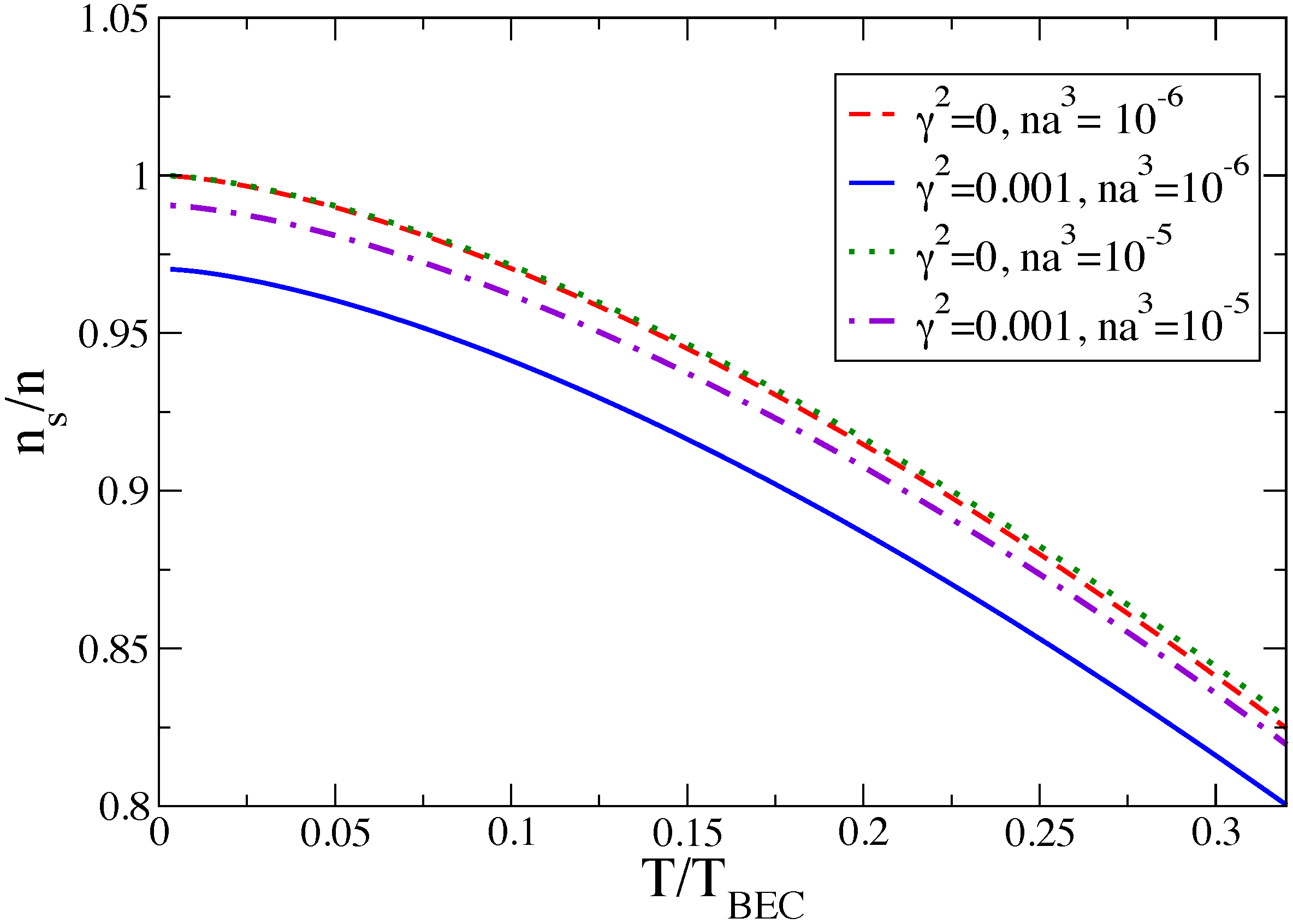
3.2. Superfluid Response and Quenched Disorder

Now, what can we say about the disorder influence on the superfluid motion of the system? Actually, within the Landau–Khalatnikov two-fluid formulation [58,59], the calculation proceeds in a similar fashion, provided that the theory is modified accordingly to the following points [50,52,54]:
  • within the Landau two-fluid model, we assume that the normal part of the system is in motion with velocity v , so τ τ i v · ;
  • Superfluid and normal parts do not exchange momentum. This means that a superflow can be imposed by means of phase twist of the field ψ ( r , τ ) , i.e., ψ exp i m v s · r / ψ with v s the superfluid velocity [60,61];
  • as a consequence of the previous points, we can redefine the chemical potential as
    μ eff = μ 1 2 m v s · ( v s 2 v ) .
The resulting Gaussian partition function (or grand potential) is formally similar to the one in Equation (27), with the replacement μ μ eff and the (inverse) Gaussian propagator given by
G 1 ( q , ω ) = i ω n + ϵ q μ + 2 g ψ 0 2 + q · ( v v s ) g ψ 0 2 g ψ 0 2 + i ω n + ϵ q μ + 2 g ψ 0 2 q · ( v v s )
whose determinant is given by
det G 1 ( q , ω n ) = E q 2 i ω n · q · ( v v s ) 2 ,
where E q as in Equation (29) with μ μ eff .
By following this prescription, the phase-twisted grand potential can be derived from Equation (33), reading
Ω dis ( μ eff , v ) th + dis = γ 2 ψ 0 2 q ϵ q μ eff + g ψ 0 2 E q 2 q · ( v v s ) 2 .
We are interested in the linear-response regime, where the density current
g = 1 L d Ω ( μ eff ( v ) , v ) v
is taken up to the first order in ( v v s ) . Therefore, we begin with an expansion of Equation (47) up to the quadratic order in q · ( v v s ) . For symmetry reasons, the linear term of this expansion is identically zero, such that we have to deal with the following equation:
Ω dis ( μ eff , v ) th + dis L d = γ 2 ψ 0 2 ( 2 π ) d d d q ϵ q μ eff + g ψ 0 2 E q 2 + 2 q 2 d ϵ q μ eff + g ψ 0 2 E q 4 ( v v s ) 2 ,
where we have made use of the identity
d d q q i q j f ( | q | ) = d 1 δ i j d d q | q | 2 f ( | q | ) .
Since the first term in the equation above depends only on μ eff and it holds μ eff v = m v s , it will be the disorder contribution to the n v s term in g . More precisely, by considering also the thermal depletion due to the quasiparticle excitations, Equation (48) reads
g = n v s + 1 d d d q ( 2 π ) d β 2 q 2 m e β E q ( e β E q 1 ) 2 + 4 γ 2 ψ 0 2 ϵ q ( ϵ q μ + g ψ 0 2 ) E q 4 ( v v s ) .
At this point, we finally replace Equation (18) for the broken-symmetry case in the equation above. A simple comparison between the resulting equation and the the two-fluid assumption g = n s v s + n n v leads us to
n n ( n 0 , T ) = β d d d q ( 2 π ) d 2 q 2 m e β E q ( e β E q 1 ) 2 + 4 d n γ ( n 0 )
with n γ ( n 0 ) as in Equation (37).
In order to understand the relevance of Equation (52), one has to remember that, in the pure system (i.e., γ = 0 ), all the particles belong to the superflow. On the contrary, a disorder potential induce a superfluid depletion also at T = 0 and, in addition, the parameter γ may act as knob to destroy the superflow since
n s ( 0 ) ( n 0 ) = n 4 d n γ ( n 0 ) .
In a similar way to the condensate fraction, we are not allowed to expand n s / n in the limit g 0 because Equation (37) is divergent in that regime. Obviously, the superfluid density can be computed from the two-fluid assumption n = n s + n n where n n is given by Equation (52). In Figure 1, we report the behaviour of the superfluid fraction in the presence of a disordered but uncorrelated external potential with γ 2 = 0.001 for two different values of the gas parameter n a s 3 . In order to highlight the crucial contribution due to disorder, we also consider the case where γ 2 = 0 . It is immediate to realize that, in pure system ( γ 2 = 0 ), the whole system is superfluid at T = 0 , while the presence of a disorder potential lowers the curves, since there is an additional depletion at T = 0 . It is also interesting to underline that, the more dilute the system, the more evident is the detachment from the pure system.

4. The Replicated Action for Superfluid Bosons

The previous section has been focused on the extension of usual field-theory techniques’ superfluid bosons subject to a random external confinement. Moreover, the whole calculation has been carried out in the quenched regime, where we effectively average over different microscopic realization of the system with a given disorder configuration.
We have already made clear that this is not the only viable strategy and that it does not handle physical realizations where, for instance, the disorder potential also has a thermal component. This means that, looking at Equation (14), it is not clear in which order integration and differentiation have to be performed. In order to overcome this ambiguity, the replica trick represents one of the most ingenious strategies. It was first developed in the context of spin glasses [62,63,64], but, in the following, we are going to detail how it can be applied to describe the role of disorder in ultracold bosonic gases.
Let us begin by considering again Equation (14). The following three hypotheses represent the starting of the replica formalism. Thus,
  • We assume that Z [ J = 0 ] = 1 , establishing a proper normalization and implying that Equation (14) has no dependence on V D in the denominator;
  • it holds O th + dis = δ log Z dis / δ J | J = 0 ;
  • for J 0 , the partition function retains its algebraic properties.
Actually, the last point is a somewhat obscure way to state that the average procedure involves functionals linear in the disorder potential, since V D has been linearly added to the action. The great advantage provided by the replica trick can be understood from the formal relations reported below:
log Z [ J ] = lim R 0 e R log Z 1 R = lim R 0 Z R 1 R
with R N . The replacement of log Z with an algebraic function of Z strongly reduces the complexity. Indeed, concerning the calculation of the expectation values, we have
O th + dis = lim R 0 δ δ J Z R R .
Actually, within the replicated formalism, expectation values can be obtained by simply considering R identical copies of the system under consideration. Concerning the functional integration, it does not alter the linear dependence of the action on the disorder field because [ exp ( d V D ) ] R = exp ( R d V D ) . Unfortunately, all this comes with a price. Looking at Equation (55), we realize that, at the end, we should perform an analytical continuation R 0 . The point is that there is no guarantee at all that the function δ J Z R dis is analytic all the way down to R = 0 [44]. This means that, from a mathematical standpoint, the replica trick is not a well-founded technique. Surprisingly, it is also true that it seems to rarely fail, at least when the disorder can be treated in a perturbative way [63,64].
Let us consider in the following the generalization of Equation (10), namely given by
P ˜ [ U D ] = exp 1 2 0 β d τ d d r γ 2 ( r , τ ) U D 2 ( r , τ ) ,
where, actually, the disorder is assumed translationally invariant in time and space. In order to implement the replica trick within the context of superfluid bosonic systems, as an alternative to Equation (19), we move to the phase-density representation, where
ψ ( r , τ ) = n 0 + π ( r , τ ) e i φ ( r , τ )
with n 0 = ψ 0 2 , ψ 0 2 being given by Equation (18). From the equation above, we deduce that n ( r , τ ) = n 0 + π ( r , τ ) and a perturbative strategy is easily implemented by assuming the smallness of density fluctuation. Thus, Equation (57) becomes
ψ ( r , τ ) n 0 1 + π ( r , τ ) 2 n 0 e i φ ( r , τ ) .
In order to understand the limitations of our approach, it is crucial to recall that n ( r , τ ) th = | ψ ( r , τ ) | 2 th , while we often set n n 0 with n 0 = | ψ ( r , τ ) th | 2 . Up to the Gaussian level, this is an acceptable approximation since π ( r , τ ) th 0 . In the regime of small fluctuations, we can expand the mean-field analysis by retaining only the quadratic terms in π ( r , τ ) and φ ( r , τ ) . The change of variables { ψ , ψ * } { π , φ } has a constant Jacobian determinant; therefore, Equation (3) reads
Z D [ π , φ ] exp 1 S g [ π , φ ]
with the periodic boundary conditions π ( r , β ) = π ( r , 0 ) and φ ( r , β ) = φ ( r , 0 ) . The smallness of fluctuations allows for extending the integration range of the phase variable from [ π , + π ] to [ , + ] . This decompactification obviously has to be addressed with particular attention when dealing with d 2 , where the enhancement of fluctuations prevents the occurring of a true long-range order and a more refined analysis is required [44,65,66,67,68]. The Gaussian action in Equation (59) is given by
S g [ π , φ ] = 0 β d τ d d r [ i π φ τ + n 0 2 ( φ ) 2 2 m + 2 ( π ) 2 8 m n 0 U D ( r , τ ) ( n 0 + π ) + 1 2 d d r π ( r , τ ) V ( | r r | ) π ( r , τ ) ] 1 2 β L d V ˜ ( 0 ) n 0 2 ,
where we have imposed Equation (18) to eliminate the dependence on the chemical potential and U D is distributed according to Equation (56). The pertubative expansion up to the terms contained in Equation (60) is equivalent to a one-loop expansion within a diagrammatic representation. Equivalently, in the second-quantization formalism, this corresponds to the Bogoliubov approximation [69].
The implementation of the replica trick requires the calculation of Z R dis . The (not-averaged) partition function is simply
Z R = D [ π , φ ] exp 1 α = 1 R S g [ π α , φ α ] ,
where S g [ π α , φ α ] is provided by Equation (60) and D [ π , φ ] = α = 1 R D [ π α , φ α ] . In case of a Gaussian disorder obeying to Equation (56), Equation (6) reads
Z R dis = D [ π , φ ] exp 1 α = 1 R S g ( pure ) [ π α , φ α ] × × D [ U D ] exp 1 2 0 β d τ d d r γ 2 ( r , τ ) U D 2 ( r , τ ) exp 1 α = 1 R S g ( coup ) [ U D , π α ] = ( ) ,
where S g ( pure ) [ π α , φ α ] is Equation (60) with U D = 0 and S g ( coup ) [ U D , π α ] is given by
S g ( coup ) [ U D , π α ] = 0 β d τ d d r U D ( r , τ ) α = 1 R π α ( r , τ ) .
The second line of Equation (62) is a Gaussian integral in U D such that
( ) = exp 1 2 0 β d τ d d r γ 2 ( r , τ ) α , β π α ( r , τ ) π β ( r , τ ) .
In this way, the replicated partition in Equation (62) results in
Z R dis = D [ π , φ ] exp 1 α = 1 R S g ( pure ) [ π α , φ α ] 1 α , β = 1 R S g ( dis ) [ π α , π β , φ α , φ β ] .
For the sake of clarity, we report below S g ( pure ) and S g ( dis ) , namely
S g ( pure ) [ π α , φ α ] = d d + 1 s i π α τ φ α + n 0 2 ( φ α ) 2 2 m + 2 ( π α ) 2 8 m n 0 + 1 2 d d r π ( r , τ ) V ( | r r | ) π ( r , τ )
S g ( dis ) [ π α , π β , φ α , φ β ] = 1 2 d d + 1 s γ 2 ( r , τ ) π α ( s ) π β ( s )
with s = ( r , τ ) . It is crucial to underline the relevance of Equation (65). Indeed, it shows that also in the presence of the simplest disorder potential ( δ -correlated both in time and space), the outlined formalism generates an effective quartic interaction between different replica indices. This fact can be understood by recalling the physical meaning of Feynman’s path. Despite its complexity, and indifferent to different replicas, the path integrals prefer to evolve towards the lowest possible potential. In other words, they have a tendency to populate the same regions of the energy landscape.
Moving to the calculation of expectation values, the replicated formalism replaces the logarithm of the partition function with, basically, Equation (65), where the Euclidean action of Equation (60) is split into Equations (66) and (67). According to Equation (55), the joint thermal and disorder average is obtained through
O th + dis = lim R 0 δ δ J 1 R Z R [ J ] = lim R 0 1 R O [ ψ α , ψ α * ] rep ,
where rep has to be intended as a thermal average over the replicated partition function in Equation (65) or, equivalently, over the action given by the sum of Equations (66) and (67), i.e.,
O rep = D [ π , φ ] O exp { 1 ( S g ( pure ) [ π , φ ] + S g ( dis ) [ π , φ ] ) } D [ π , φ ] exp { 1 ( S g ( pure ) [ π , φ ] + S g ( dis ) [ π , φ ] ) } .
It is useful to expand the fields in Fourier series such that Equation (66) reads
S g ( pure ) [ π α , φ α ] = 1 2 β L d q n χ α T ( q , ω n ) M 1 ( q , ω n ) χ α ( q , ω n ) ,
where we have defined the vector χ α as χ α ( q , ω n ) T φ α ( q , ω n ) ; π α ( q , ω n ) The pure inverse propagator in Equation (70) is given by
M 1 ( q , ω n ) = n 0 2 q 2 m ω n + ω n 2 q 2 4 m n 0 + V ˜ ( q ) .
On the other hand, for Equation (63), we have now
S g ( dis ) [ π α , π β , φ α , φ β ] = 1 2 β L d q n γ 2 ( q , ω n ) π α * ( q , ω n ) π β ( q , ω n ) .
The equation above can be decomposed in its diagonal and off-diagonal contributions, leading us to the final equation for the Euclidean action of Gaussian fluctuations. By renaming Q = ( q , ω n ) and using the fact that x ( Q ) = x * ( Q ) , we have
S g ( rep ) [ π , φ ] = 1 2 β L d Q X ( Q ) M 1 ( Q ) X ( Q ) .
In the equation above, the sum over the replicas is encoded in the ( R × 2 ) -dimensional column vector
X ( Q ) = χ 1 ( Q ) χ 2 ( Q ) χ R ( Q ) .
The R × 2 matrix M 1 ( Q ) in Equation (73) is built as
M 1 ( Q ) = M ˜ 1 ( Q ) B ( γ ) B ( γ ) B ( γ ) M ˜ 1 ( Q ) B ( γ ) B ( γ ) B ( γ ) B ( γ ) B ( γ ) M ˜ 1 ( Q )
with the generating blocks
M ˜ 1 ( Q ) = n 0 2 q 2 m ω n + ω n 2 q 2 4 m n 0 + V ˜ ( q ) γ 2 ( q , ω n ) ,
B ( γ ) = 0 0 0 γ 2 ( q , ω n ) .

5. Correlation Functions in the Replicated Formalism

As detailed in Appendix A, the matrix M in Equation (75) is diagonalized by a well-known unitary transformation, reading
M ˜ 1 ( Q ) = diag M ˜ R 1 ( Q ) , M ˜ 1 ( Q ) , , M ˜ 1 ( Q ) R 1 times
with
M R 1 ( Q ) = n 0 2 q 2 m ω n + ω n 2 q 2 4 m n 0 + V ˜ ( q ) R γ 2 ( q , ω n ) .
Up to this level of approximation, correlation functions are specified by the entries of the fluctuation propagator. For the pure system, by assuming translational invariance both in time and space, we have
χ j ( q , ω n ) χ k ( q , ω n ) th = M j k ( q , ω n ) δ ( q + q ) β δ n , n .
On the other hand, according to Equation (68), the replicated formalism provides both the disorder and the thermal average at the same time. For instance, concerning the density-density correlation function, we have
π * ( q , ω n ) π ( q , ω n ) dis + th = lim R 0 1 R α = 1 R π α ( q , ω n ) π α ( q , ω n ) S g ( rep ) = lim R 0 1 R ( R 1 ) n 0 3 q 2 / m 2 ω n 2 + E q 2 + n 0 2 q 2 / m 2 ω n 2 + E q 2 R γ 2 ( q , ω n ) n 0 2 q 2 m δ ( q + q ) β δ n , n = n 0 3 q 2 / m 2 ω n 2 + E q 2 + γ 2 ( q , ω n ) n 0 2 q 2 q 2 / m 2 ω n 2 + E q 2 2 ω n 2 + E q δ ( q + q ) β δ n , n ,
where the final result is obtained by expanding the second line up to the first order in R. Moreover, we have
E q = ϵ q ϵ q + 2 n 0 V ˜ ( q ) ,
nothing else than Equation (29) with the saddle-point replacement μ = V ˜ ( 0 ) n 0 . The remaining correlations are computed in the same way, leading to
φ * ( q , ω n ) φ ( q , ω n ) dis + th = m E q 2 / ( n 0 q 2 ) 2 ω n 2 + E q 2 + 2 ω n ω n 2 ω n 2 + E q 2 2 ω n 2 + E q γ 2 ( q , ω n ) δ ( q + q ) β δ n , n , φ * ( q , ω n ) π ( q , ω n ) dis + th = 2 ω n 2 ω n 2 + E q 2 + n 0 3 q 2 ω n / m 2 ω n 2 + E q 2 2 ω n 2 + E q γ 2 ( q , ω n ) δ ( q + q ) β δ n , n .
Besides the phase and density correlators, one of the most important correlation functions is the current one, defined as
C i j ( r , τ ; r , τ ) = m 1 g i ( r , τ ) g j ( r , τ ) g i ( r , τ ) g j ( r , τ ) ,
where the notation represents, for now, a general average procedure. In the phase-density representation, from Equation (57), it is easy to verify that the current density g = ( n 0 + π ) φ / m . Thus, by making use of the Wick theorem [70] to disentagle the four-field correlator in Equation (84), in the Fourier space, one obtains [35]
C i j ( q , ω n ; q , ω n ) = 2 m n 0 2 q i q j φ ( q , ω n ) φ ( q , ω n ) + 1 ( β L d ) 2 k , ω m k , ω m k i k j [ π ( q k , ω l m ) π ( q k , ω l m ) φ ( k , ω m ) φ ( k , ω m ) + + π ( k q , ω m l ) φ ( k , ω m ) π ( k q , ω m l ) φ ( k , ω m ) ] .
Thanks to the replica trick, the disorder contribution is taken into account by considering the correlators over the replicated Gaussian action, namely Equations (81) and (83).
The current response function in Equation (85) is crucial since it encodes the superfluid character of the system. This point is clarified by noticing that C i j is a 2-rank tensor, so it can be decomposed in its longitudinal and transverse components by means of the projectors P i j L = q i q j / q 2 and P i j T = δ i j P i j L . It has been shown (see [71,72] for a pedagogical review) that the static limit of transverse component of Equation (85) C i j T ( q , ω n ) ( d 1 ) 1 i j P i j T ( q , ω n ) C i j ( q , ω n ) / corresponds to the normal component of the system. By replacing the replicated correlator given by Equations (81) and (83) into Equation (85), after burdensome (but standard) algebra, we find
n n = lim q 0 C T ( q , 0 ) th + dis = 1 d β L d k , ω m 2 k 2 m E k 2 2 ω m 2 ( 2 ω m 2 + E q 2 ) 2 + n 0 2 k 2 m 2 E k 2 3 2 ω m 2 ( 2 ω m 2 + E k 2 ) 3 γ 2 ( k , ω m ) .
When the time scale of the disorder potential is frozen, i.e., for
γ 2 ( q , ω n ) = γ 2 ( q ) β δ n , 0 ,
Equation (86) becomes
n n ( n 0 , T ) = β d d d q ( 2 π ) d 2 q 2 m e β E q ( e β E q 1 ) 2 + 4 n 0 d d d q ( 2 π ) d 2 q 2 2 m 2 γ 2 ( q ) E q 4 .
With the further simplification of a constant disorder correlator γ 2 , the equation above equates to Equation (52). Thus, Equation (88) reduces correctly to the quenched disorder regime and agrees with results reported in [34,35,47].
In order to compute the condensate depletion through the replicated correlators in Equations (81) and (83), we rely upon the equation [70]
n = n 0 + 1 β d d q ( 2 π ) d n e i ω n 0 + ψ ( r , τ ) ψ * ( r , τ ) n 0 .
Following the phase-density representation in Equation (57), we expand the fields ψ and ψ * up to the linear order in the fluctuations ψ ( r , τ ) n 0 [ 1 + π ( r , τ ) / ( 2 n 0 ) + i φ ( r , τ ) ] , such that the resulting correlators in Equation (89) are Gaussian. In the Fourier space, we have
ψ ( q , ω n ) ψ * ( q , ω n ) n 0 1 4 n 0 π π i 2 π φ + i 2 φ π + n 0 φ φ ,
where the prime signal the dependence on Q = ( q , τ ) and, similarly to Equation (84), corresponds to a general average procedure. In order to include the disorder contribution, one simply has to consider the replicated correlators in Equations (81) and (83), where space-time translational invariance is restored by assuming Equation (80).
We then have
n = n 0 + d d q ( 2 π ) d [ ϵ q + n 0 V ˜ ( q ) 2 E q 1 2 + ϵ q + n 0 V ˜ ( q ) E q 1 e β E q 1 + n 0 β m ϵ q 2 2 ω m ( 2 ω m 2 + E q 2 ) 2 γ 2 ( q , ω m ) ] .
The first line represents the contribution coming from the pure system, reading Equation (40) at T = 0 K . On the other hand, the second line accounts for the disorder contribution. For a point-like frozen disorder as in Equation (87), one can verify that
n γ ( n 0 ) = n 0 d d q ( 2 π ) d 2 q 2 2 m 2 γ 2 ( q ) E q 4 .
By comparing the equation above and Equation (88), at zero-temperature, the disorder contribution to the condensate depletion and the normal component of the system are deeply related, namely
n γ ( n 0 ) = d 4 n n ( n 0 , T = 0 ) .

6. Conclusions and Future Perspectives

In this review, we have reviewed the crucial aspects of a field-theory approach to superfluid bosons moving in a random environment. Within the powerful framework of functional integration, we have recovered the important result on the superfluid and condensate depletion in the presence of an external disorder [33,34,47]. Moreover, we have shown how the theoretical description can be generalized beyond the assumption of a static external disorder by using the replicated formalism [39]. Obviously, our pedagogical overview has to leave out other interesting and crucial issues. For instance, we have pointed out in Section 3 that our perturbative approach lacks self-consistency, since we are expanding above a uniform background also in the presence of an external potential. In order to overcome this point, in [42,43], the authors present a self-consistent implementation relying upon the Hartee–Fock mean-field theory within the replica formalism. Moreover, our review does not include any discussion about the eventual occurring of the superfluid-glass transition in three or lower dimensions. This is a crucial topic, deserving a separate investigation. Numerical simulations based on quantum Monte Carlo methods are likewise important, since they are ab initio calculation and may shed light on unexpected effects. For instance, in [73], the non-trivial relation between superfluidity and condensation is numerically investigated, while, in [74], the worm algorithm provides an estimation for critical exponents of the superfluid-glass transition in two-dimensions.
Another promising line of research concerns the possibility that disorder does not always act in a parasitic way, generating, on the contrary, surprising dynamical effects. In the context of condensed matter theory, one of the most striking example is given by the quantum Hall transition [75], where impurity scattering plays a crucial role. On the other hand, very recently, it was shown that a certain degree of random fluctuations, such as thermal noise, may enhance the transport properties of a particles ensemble. While Anderson localization [21] acts to halt the flow of a certain quantity, in [76,77], the authors observe a boosting of transport through optical fibers and superconducting circuits. The reason is the so-called environment-assisted quantum transport, which relies crucially upon the presence of a certain degree of disorder. Indeed, while the coherence of the system is reduced by propagating in a disordered medium, this also reduces the possibility of destructive interference responsible for Anderson localization.
This phenomenon can pave the way to novel interesting protocol to engineer more efficient quantum devices, by tuning the coupling with the environment to enhance the transport of a desired quantity. Recent experimental confirmations have been produced by using a one-dimensional array of trapped ions [78]. Thus, it would be extremely interesting to review to effect in the context of ultracold atoms, both from an experimental and theoretical point of view.

Author Contributions

Both A.C. and L.S. have contributed to the development and and the writing process of the present manuscript.

Funding

L.S. acknowledges partial support of the FFABR grant of the Italian Ministry of Education, University and Research.

Acknowledgments

A.C. thanks Andrea Tononi for useful discussions and meaningful insight on the manuscript.

Conflicts of Interest

The authors declare no conflict of interest.

Appendix A. Diagonalization of a Block Circulant Matrix

It is possible to perform a block diagonalization of M 1 in Equation (75) by noticing its circulant structure. Indeed, G 1 is generated by cyclically permuting the elements (in this case 2 × 2 matrices) of its first row. In this sense, we can formally write down
M 1 ( Q ) = Circ M ˜ 1 ( Q ) , B ( Q ) , , B ( Q ) R 1 times .
It has been shown [79,80] that, given R the number of the generating matrices and M their dimension, every block circulant matrix A is block diagonalized by the same unitary transformation. Indeed, one can verify that
( E R 1 M ) A ( E R 1 M ) = diag { Λ 1 , , Λ R } ,
where the Λ j are the 2 × 2 eigenblocks, specified by Λ j = M 1 + α = 1 R 1 B w R α j . The ⊗ symbol denotes the direct product of the two matrices. In Equation (A2), the key ingredient is the Fourier matrix, defined as
E R = 1 R 1 1 1 1 1 w R w R 2 w R R 1 1 w R 2 w R 4 w R 2 ( R 1 ) 1 w R R 1 w R 2 ( R 1 ) w R ( R 1 ) 2
with w R = exp ( 2 π i / R ) the fundamental root of the unity.

References

  1. Anderson, M.H.; Ensher, J.R.; Matthews, M.R.; Wieman, C.E.; Cornell, E.A. Observation of Bose–Einstein Condensation in a Dilute Atomic Vapor. Science 1995, 269, 5221. [Google Scholar] [CrossRef]
  2. Davis, K.B.; Mewes, M.O.; Andrews, M.R.; van Druten, N.J.; Durfee, D.S.; Kurn, D.M.; Ketterle, W. Bose–Einstein Condensation in a Gas of Sodium Atoms. Phys. Rev. Lett. 1995, 75, 3969. [Google Scholar] [CrossRef] [PubMed]
  3. Pethick, C.J.; Smith, H. Bose–Einstein Condensation in Dilute Gases; Cambridge University Press: Cambridge, UK, 2011. [Google Scholar]
  4. Langen, T.; Geiger, R.; Schmiedmayer, J. Ultracold atoms out of equilibrium. Annu. Rev. Condens. Matt. Phys. 2015, 6, 201–217. [Google Scholar] [CrossRef]
  5. Fisher, M.P.A.; Weichman, P.B.; Grinstein, G.; Fisher, D.S. Boson localization and the superfluid–insulator transition. Phys. Rev. B 1989, 40, 546. [Google Scholar] [CrossRef]
  6. Greiner, M.; Mandel, O.; Esslinger, T.; Hänsch, T.W.; Bloch, I. Quantum phase transition from a superfluid to a Mott insulator in a gas of ultracold atoms. Nature 2002, 415, 39–44. [Google Scholar] [CrossRef] [PubMed]
  7. Giamarchi, T. Quantum Physics in One Dimensions; Clarendon Press: Oxford, UK, 2003. [Google Scholar]
  8. Hadzibabic, Z.; Dalibard, J. Two-Dimensional Bose Fluids: An Atomic Physics Perspective. Rivista del Nuovo Cimento 2011, 34, 389. [Google Scholar] [CrossRef]
  9. Paredes, B.; Widera, A.; Murg, V.; Mandel, O.; Folling, S.; Cirac, I.; Shlyapnikov, G.V.; Hänsch, T.W.; Bloch, I. Tonks–Girardeau gas of ultracold atoms in an optical lattice. Nature 2004, 429, 277. [Google Scholar] [CrossRef]
  10. Kinoshita, T.; Wenger, T.; Weiss, D.S. Observation of a One-Dimensional Tonks–Girardeau Gas. Science 2004, 305, 1125. [Google Scholar] [CrossRef] [PubMed]
  11. Hadzibabic, Z.; Krüger, P.; Cheneau, M.; Battelier, B.; Dalibard, J. Berezinskii-Kosterlitz- ouless crossover in a trapped atomic gas. Nature 2006, 441, 1118. [Google Scholar] [CrossRef]
  12. Schweikhard, V.; Tung, S.; Cornell, E.A. Vortex proliferation in the Berezinskii-Kosterlitz- ouless regime on a two-dimensional lattice of Bose–Einstein condensates. Phys. Rev. Lett. 2007, 99, 030401. [Google Scholar] [CrossRef] [PubMed]
  13. Neuenhahn, C.; Marquardt, F. Quantum simulation of expanding space–time with tunnel-coupled condensates. New J. Phys. 2015, 17, 125007. [Google Scholar] [CrossRef]
  14. Fialko, O.; Opanchuk, B.; Sidorov, A.I.; Drummond, P.D.; Brand, J. The universe on a table top: Engineering quantum decay of a relativistic scalar field from a metastable vacuum. J. Phys. B At. Mol. Opt. Phys. 2017, 50, 024003. [Google Scholar] [CrossRef]
  15. Braden, J.; Johnson, M.C.; Peiris, H.V.; Weinfurtner, S. Towards the cold atoms analog of the false vacuum. J. High Energy Phys. 2018, 2018, 14. [Google Scholar] [CrossRef]
  16. Liberati, S.; Visser, M.; Weinfurtner, S. Analogue quantum gravity phenomenology from a two-component Bose–Einstein condensate. Class. Quant. Grav. 2006, 23, 3129. [Google Scholar] [CrossRef]
  17. Kurkcuoglu, D.M.; de Melo, C.S. Unconventional color superfluidity in ultra-cold fermions: Quintuplet pairing, quintuple point and pentacriticality. arXiv, 2018; arXiv:1811.07272. [Google Scholar]
  18. Kamenev, A. Many-body theory of non-equilibrium systems. In Nanophysics: Coherence and Transport; Elsevier: Amsterdam, The Netherlands, 2005; pp. 177–246. [Google Scholar]
  19. Ma, M.; Lee, P.A. Localized superconductors. Phys. Rev. B 1985, 32, 5658. [Google Scholar] [CrossRef]
  20. Ma, M.; Halpering, B.I.; Lee, P.A. Strongly disordered superfluids: Quantum fluctuations and critical behavior. Phys. Rev. B 1986, 34, 3136. [Google Scholar] [CrossRef]
  21. Anderson, P.W. Absence of diffusion in certain random lattices. Phys. Rev. 1959, 109, 1492. [Google Scholar] [CrossRef]
  22. Damski, B.; Zakrzewski, J.; Santos, L.; Zoller, P.; Lewenstein, M. Atomic Bose and Anderson Glasses in Optical Lattices. Phys. Rev. Lett. 2003, 91, 080403. [Google Scholar] [CrossRef]
  23. Schulte, T.; Drenkelforth, S.; Kruse, J.; Ertmer, W.; Arlt, J.; Sacha, K.; Zakrzewski, J.; Lewenstein, M. Routes Towards Anderson-Like Localization of Bose–Einstein Condensates in Disordered Optical Lattices. Phys. Rev. Lett. 2005, 95, 170411. [Google Scholar] [CrossRef]
  24. Billy, J.; Josse, V.; Zuo, Z.; Bernard, A.; Hambrecht, B.; Lugan, P.; Clement, D.; Sanchez-Palencia, L.; Bouyer, P.; Aspect, A. Direct Observation of Anderson Localization of Matter-Waves in a Controlled Disorder. Nature 2008, 453, 891. [Google Scholar] [CrossRef]
  25. Roati, G.; D’Errico, C.; Fallani, L.; Fattori, M.; Fort, C.; Zaccanti, M.; Modugno, G.; Modugno, M.; Inguscio, M. Anderson Localization of a Non-Interacting Bose–Einstein Condensate. Nature 2008, 453, 895. [Google Scholar] [CrossRef]
  26. Dainty, J.C. An introduction to Gaussian speckle. Proc. SPIE 1980, 243, 2–8. [Google Scholar]
  27. Goodman, J.W. Speckle Phenomena in Optics: Theory and Applications; Roberts & Company: Englewood, CO, USA, 2010. [Google Scholar]
  28. Lye, J.E.; Fallani, L.; Modugno, M.; Wiersma, D.S.; Fort, C.; Inguscio, M. A Bose–Einstein condensate in a random potential. Phys. Rev. Lett. 2005, 95, 070401. [Google Scholar] [CrossRef]
  29. Clément, D.; Varón, A.F.; Hugbart, M.; Retter, J.A.; Bouyer, P.; Sanchez-Palencia, L.; Gangardt, D.M.; Shlyapnikov, G.V.; Aspect, A. Suppression of Transport of an Interacting Elongated Bose–Einstein Condensate in a Random Potential. Phys. Rev. Lett. 2005, 95, 170409. [Google Scholar] [CrossRef]
  30. Ghabour, M.; Pelster, A. Bogoliubov theory of dipolar Bose gas in a weak random potential. Phys. Rev. A 2014, 90, 063636. [Google Scholar] [CrossRef]
  31. Stoof, H.T.C.; Dickerscheid, D.B.M.; Gubbels, K. Ultracold Quantum Fields; Springer: Dordrecht, The Netherlands, 2009. [Google Scholar]
  32. Salasnich, L.; Toigo, F. Zero-point energy of ultracold atoms. Phys. Rep. 2016, 640, 1–29. [Google Scholar] [CrossRef]
  33. Huang, K.; Meng, H.-F. Hard-Sphere Bose Gas in Random External Potential. Phys. Rev. Lett. 1992, 69, 644. [Google Scholar] [CrossRef]
  34. Giorgini, S.; Pitaevskii, L.; Stringari, S. Effects of disorder in a dilute Bose gas. Phys. Rev. B 1994, 49, 18. [Google Scholar] [CrossRef]
  35. Taüber, U.; Nelson, D.R. Superfluid bosons and flux liquids: Disorder, thermal fluctuations, and finite-size effects. Phys. Rep. 1997, 289, 157. [Google Scholar] [CrossRef]
  36. Lopatin, A.V.; Vinokur, V.M. Thermodynamics of the Superfluid Dilute Bose Gas with Disorder. Phys. Rev. Lett. 2002, 88, 235503. [Google Scholar] [CrossRef] [PubMed]
  37. Falco, G.M.; Pelster, A.; Graham, R. Thermodynamics of a Bose–Einstein condensate with weak disorder. Phys. Rev. A 2007, 75, 063619. [Google Scholar] [CrossRef]
  38. Giamarchi, T.; Schulz, H.J. Anderson localization and interactions in one-dimensional metals. Phys. Rev. B 1988, 37, 325. [Google Scholar] [CrossRef]
  39. Navez, P.; Pelster, A.; Graham, R. Bose condensed gas in strong disorder potential with arbitrary correlation length. Appl. Phys. B 2007, 86, 395–398. [Google Scholar] [CrossRef]
  40. Yukalov, V.I.; Graham, R. Bose–Einstein condensed systems in random potentials. Phys. Rev. A 2007, 75, 023619. [Google Scholar] [CrossRef]
  41. Falco, G.M.; Nattermann, T.; Pokrovsky, V.L. Weakly interacting Bose gas in a random environment. Phys. Rev. B 2009, 80, 104515. [Google Scholar] [CrossRef]
  42. Khellil, T.; Balaz, A.; Pelster, A. Analytical and numerical study of dirty bosons in a quasi-one-dimensional harmonic trap. New J. Phys. 2016, 18, 063003. [Google Scholar] [CrossRef]
  43. Khellil, T.; Pelster, A. Hartree-Fock Mean-Field Theory for Trapped Dirty Bosons. J. Stat. Mech. 2016, 2016, 063301. [Google Scholar] [CrossRef]
  44. Altland, A.; Simons, B. Condensed Matter Field Theory; Cambridge University Press: Cambridge, UK, 2010. [Google Scholar]
  45. Hertz, J. Disordered Systems. Phys. Scr. 1985, 1985, 1. [Google Scholar] [CrossRef]
  46. Nelson, D.R.; le Doussal, P. Correlations in flux liquids with weak disorder. Phys. Rev. B 1990, 42, 16. [Google Scholar] [CrossRef]
  47. Schakel, A.M.J. Quantum critical behavior of disordered superfluids. Phys. Lett. A 1997, 224, 287. [Google Scholar] [CrossRef]
  48. Lubensky, T.C. Critical properties of the random-spin model from the ϵ-expansion. Phys. Rev. B 1975, 11, 9. [Google Scholar] [CrossRef]
  49. Grinstein, G.; Luther, A. Applications of the renormalization group to phase transition in disordered systems. Phys. Rev. B 1976, 13, 3. [Google Scholar] [CrossRef]
  50. Schakel, A.M.J. Boulevard of Broken Symmetries: Effective Field Theories of Condensed Matter; World Scientific: Singapore, 2008. [Google Scholar]
  51. Astrakharchik, G.E.; Boronat, J.; Casulleras, J.; Kurbakov, I.L.; Lozovik, Y.E. Equation of state of a weakly interacting two-dimensional Bose gas studied at zero temperature by means of quantum Monte Carlo methods. Phys. Rev. A 2009, 79, 051602. [Google Scholar] [CrossRef]
  52. Tononi, A.; Cappellaro, A.; Salasnich, L. Condensation and superfluidity of dilute Bose gases with finite-range interaction. New J. Phys. 2018, 20, 125007. [Google Scholar] [CrossRef]
  53. Salasnich, L. Nonuniversal Equation of State of the Two-Dimensional Bose Gas. Phys. Rev. Lett. 2017, 118, 130402. [Google Scholar] [CrossRef]
  54. Tononi, A. Zero-temperature equation of state of a two-dimensional bosonic quantum fluid with finite-range interaction. Condens. Matter 2019, 4, 20. [Google Scholar] [CrossRef]
  55. Wehr, J.; Niederberger, A.; Sanchez-Palencia, L.; Lewenstein, M. Disorder versus the Mermin-Wagner-Hohenberg effect: From classical spin systems to ultracold atomic gases. Phys. Rev. B 2006, 74, 224448. [Google Scholar] [CrossRef]
  56. Boudjemaa, A.; Shlyapnikov, G.V. Two-dimensional dipolar Bose gas with the roton-maxon excitation spectrum. Phys. Rev. A 2013, 87, 025601. [Google Scholar] [CrossRef]
  57. Boudjemaa, A. Two-dimensional dipolar bosons with weak disorder. Phys. Lett. A 2015, 379, 2484–2487. [Google Scholar] [CrossRef]
  58. Landau, L.D.; Lifshitz, E.M. Statistical Physics 2; Pergamon Press: Oxford, UK, 1987. [Google Scholar]
  59. Khalatnikov, I.M. An Introduction to the Theory of Superfluidity; Westwiew Press: Oxford, UK, 2000. [Google Scholar]
  60. Fisher, M.E.; Barber, M.N.; Jasnow, D. Helicity, Modulus, Superfluidity and Scaling in Isotropic Systems. Phys. Rev. A 1973, 8, 1111. [Google Scholar] [CrossRef]
  61. Taylor, E.; Griffin, A.; Fukushima, N.; Ohashi, Y. Pairing fluctuations and the superfluid density through the BCS-BEC crossover. Phys. Rev. A 2006, 74, 063626. [Google Scholar] [CrossRef]
  62. Edwards, S.F.; Anderson, P.W. Theory of spin glasses. J. Phys. F 1975, 5, 965–974. [Google Scholar] [CrossRef]
  63. Mezard, M.; Parisi, G.; Virasoro, M. Spin Glass Theory and Beyond: An Introduction to the Replica Method and Its Applications; World Scientific: Singapore, 1987. [Google Scholar]
  64. Parisi, G. Glasses, replicas and all that. In Les Houches—Ecole d’ été de Physique Théorique; Elsevier: Amsterdam, The Netherlands, 2004; Volume 77. [Google Scholar]
  65. Mermin, N.D.; Wagner, H. Absence of Ferromagnetism or antiferromagnetism in one- or two- dimensional isotropic heisenberg models. Phys. Rev. Lett. 1966, 17, 1133. [Google Scholar] [CrossRef]
  66. Hohenberg, P.C. Existence of Long-Range Order in One and Two Dimensions. Phys. Rev. 1967, 158, 383. [Google Scholar] [CrossRef]
  67. Villain, J. Theory of one- and two-dimensional magnets with an easy magnetization plane. II. The planar, classical, two-dimensional magnet. J. Phys. 1975, 36, 581. [Google Scholar] [CrossRef]
  68. José, J.V.; Kadanoff, L.P.; Kirkpatrick, S.; Nelson, D.R. Renormalization, vortices and symmetry-breaking perturbations in the two-dimensional planar model. Phys. Rev. B 1977, 16, 1217. [Google Scholar] [CrossRef]
  69. Andersen, J.O. Theory of the weakly interacting Bose gas. Rev. Mod. Phys. 2004, 76, 599. [Google Scholar] [CrossRef]
  70. Fetter, A.L.; Walecka, J.D. Quantum Theory of Many-Particle Systems; Dover Publications: New York, NY, USA, 2003. [Google Scholar]
  71. Baym, G. Microscopic Description of Superfluidity. In Mathematical Methods in Solid State and Superfluid Theory; Springer: Berlin/Heidelberg, Germany, 1967. [Google Scholar]
  72. Ueda, M. Fundamentals and New Frontiers in Bose–Einstein Condensations; World Scientific: Singapore, 2010. [Google Scholar]
  73. Astrakharchik, G.E.; Boronat, J.; Casulleras, J.; Giorgini, S. Superfluidity versus Bose–Einstein condensation in a Bose gas with disorder. Phys. Rev. A 2002, 66, 023603. [Google Scholar] [CrossRef]
  74. Ng, R.; Sorensen, E.S. Quantum Critical Scaling of Dirty Bosons in Two Dimensions. Phys. Rev. Lett. 2015, 114, 255701. [Google Scholar] [CrossRef]
  75. Pruisken, A.M.M. Field theory, scaling and the localization problem. In The Quantum Hall Effect; Springer-Verlag: Berlin/Heidelberg, Germany, 1987. [Google Scholar]
  76. Viciani, S.; Lima, M.; Bellini, M.; Caruso, F. Observation of noise-assisted transport in an all-optical cavity-based network. Phys. Rev. Lett. 2015, 115, 083601. [Google Scholar] [CrossRef]
  77. Potocnik, A.; Bargerbos, A.; Schröder, F.A.; Khan, S.A.; Collodo, M.C.; Gasparinetti, S.; Salathé, Y.; Creatore, C.; Eichler, C.; Türeci, H.E.; et al. Studying light-harvesting models with superconducting circuits. Nat. Commun. 2018, 9, 904. [Google Scholar] [CrossRef]
  78. Maier, C.; Brydges, T.; Jurcevic, P.; Trautmann, N.; Hempel, C.; Lanyon, B.P.; Hauke, P.; Blatt, R.; Roos, C.F. Environment-Assisted Quantum Transport in a 10-qubit Network. Phys. Rev. Lett. 2019, 122, 050501. [Google Scholar] [CrossRef]
  79. Davis, P.J. Circulant Matrices, 2nd ed.; American Mathematical Society: New York, NY, USA, 1979. [Google Scholar]
  80. Olson, B.; Shaw, S.; Shi, C.; Pierre, C.; Parker, R. Circulant Matrices and Their Application to Vibration Analysis. Appl. Mech. Rev. 2014, 66, 040803. [Google Scholar] [CrossRef]
Figure 1. Plot of superfluid fraction in presence and absence of an uncorrelated disordered potential. The curve are derived from the two-fluid assumption n = n s + n n , with the normal contribution n n given by Equation (52). The temperatures are in units of T BEC = 2 π 2 n 2 / 3 / ( m k B ζ ( 3 / 2 ) 2 / 3 ) , i.e., the condensation temperature of an ideal Bose gas. The solid blue line and the dot-dashed violet one represent the behaviour of n s / n in the presence of a disordered potential with γ 2 = 0.001 for two different values of the gas parameter n a s 3 = 10 6 and 10 5 , respectively. For the same values of n a s 3 , the dashed red line and the dotted green correspond the case where there is no disorder contribution ( γ 2 = 0 ).
Applsci 09 01498 g001

