An Ultrashort-Term Net Load Forecasting Model Based on Phase Space Reconstruction and Deep Neural Network

Abstract

Recently, a large number of distributed photovoltaic (PV) power generations have been connected to the power grid, which resulted in an increased fluctuation of the net load. Therefore, load forecasting has become more difficult. Considering the characteristics of the net load, an ultrashort-term forecasting model based on phase space reconstruction and deep neural network (DNN) is proposed, which can be divided into two steps. First, the phase space reconstruction of the net load time series data is performed using the C-C method. Second, the reconstructed data is fitted by the DNN to obtain the predicted value of the net load. The performance of this model is verified using real data. The accuracy is high in forecasting the net load under high PV penetration rate and different weather conditions.

1. Introduction

In recent years, an increasing number of photovoltaic (PV) power generations have been connected to the distribution network. The use of new energy brings huge benefits to human beings. However, it also has negative impacts on the power grid while improving the environment. The PV power is greatly influenced by weather conditions and fluctuates with the change in irradiance. To ensure the quality of the power supply and safe operation of the power system, it is necessary to maintain equal amounts of power generation and power consumption in the power system. The power load forecasting is an indispensable mean of maintaining this dynamic balance. In addition, power load forecasting is also of great significance for the planning and scheduling of power systems and the planning of power maintenance. However, the fluctuations in PV power can cause fluctuations in the load when many PV systems are connected. Therefore, load forecasting will become more difficult.

Generally, load forecasting can be divided into long-term forecasting, medium-term forecasting, short-term forecasting, and ultrashort-term forecasting [1]. Recently, many systematic and fruitful studies on traditional load forecasting have been conducted. The load forecasting methods mainly include the similar day prediction method [2,3], time series prediction method [4,5], expert system [6,7], and regression analysis method [8,9]. Artificial intelligence and machine learning algorithm are types of prediction methods that have rapidly developed in recent years. Support vector regression (SVR) [10], relevance vector regression (RVR) [11], artificial neural network (ANN) [12], deep neural network (DNN) [13], and their improved hybrid algorithms [14] have been applied in the field of load forecasting. In Moon et al. [15], the random forest and multilayer perceptron are combined to predict the daily electrical load. In Nazar et al. [16], the wavelet and Kalman machines, Kohonen self-organizing map (SOM), multi-layer perceptron artificial neural network (MLP-ANN) and adaptive neuro-fuzzy inference system (ANFIS) are used to establish a hybrid three-stage forecasting model. In Zhang et al. [17], a short-term power load forecasting method with wavelet neural network (WNN) and an adaptive mutation bat optimization algorithm (AMBA) are proposed. Liang et al. [18] propose a hybrid model that combines the empirical mode decomposition (EMD), minimal redundancy maximal relevance (mRMR), general regression neural network (GRNN), and fruit fly optimization algorithm (FOA). In Dai et al. [19], a load forecasting model is proposed based on the complete ensemble empirical mode decomposition (EEMD) with adaptive noise and support vector machine (SVM), which is optimized by the modified grey wolf optimization (MGWO) algorithm.

Since traditional load data are typically in hours as the smallest unit, short-term and ultrashort-term forecasts are often not strictly distinguished. With the large-scale access of distributed PV, the short-term load forecasting usually in hours cannot satisfy the requirements of the real-time safety analysis. For the real-time safety analysis of power systems and the reliable operation of economic dispatch, a more detailed ultrashort-term prediction is required. Considering the volatility of the distributed PV power generation and the real-time requirements of the ultrashort-term prediction, the PV power should also be considered a load and merged with the traditional load to form a net load [20,21,22]. Because the net load is a set of nonlinear time series with large volatility, in this paper, the phase space reconstruction of net load data is first performed to project the data into the moving point with certain regularity of the trajectory in the phase space. Then, the excellent nonlinear fitting ability of the deep neural network is used to fit the moving point trajectory to obtain the final prediction value. Finally, the actually measured load data is applied to verify the prediction effectiveness and prediction effect of the model under different weather conditions. The phase space is a tool to feature a dynamic system that is reconstructed from a univariate or multivariate time series [23], which is widely used in forecasting models. The DNN is the development of the traditional ANN and suitable for net load forecasting because the nonlinear fitting ability is strengthened [24]. The high accuracy in forecasting the net load under high PV penetration rate and different weather conditions is verified using real data. The contribution of this paper can be summarized as follows:

• The bus load prediction model is established considering distributed PV power supply. The prediction results are necessary guidance for the power grid dispatching, which is conducive to the improvement of PV consumption.
• The phase space reconstruction is used to process bus load data, and one-dimensional time series data are inversely constructed into the phase space structure of the original system, which can better describe the dynamic characteristics and adapt to the strong fluctuation of the bus load.
• Levenberg-Marquardt back propagation (LMBP) algorithm is used to train DNN, which accelerates the training speed. Compared with the single hidden layer neural network, DNN can fit the historical data better and significantly improve the accuracy of ultrashort-term load forecasting.

2. Fundamental of Phase Space Reconstruction and Deep Neural Network

2.1. Phase Space Reconstruction

Phase space reconstruction is a method proposed by Takens to analyze the time series. The basic idea of the phase space reconstruction is to regard the time series as a component produced by a certain nonlinear dynamic system. The equivalent high-dimensional phase space of the power system can be reconstructed by the variation law of the component. Among them, the key to reconstruction is to determine the optimal embedding dimension m_opt and delay t_opt.

In this paper, the optimal embedding dimension m_opt and delay t_opt are simultaneously obtained by the C-C method. If a set of time series is $\mathit{x}=\left\{x_1,x_2\cdots x_N\right\}$, the embedding dimension is m, and the time delay is t, then the set of points in the reconstructed phase space can be expressed by Formula (1), where $M=N-(m-1)t$ [25].

$$\left[\begin{array}{c}{\mathit{X}}_1\\ {\mathit{X}}_2\\ ⋮\\ {\mathit{X}}_M\end{array}\right]=\left[\begin{array}{cccc}{x}_1& x_{1+t}& \cdots & x_{1+(m-1)t}\\ x_2& x_{2+t}& \cdots & x_{2+(m-1)t}\\ ⋮& ⋮& \cdots & ⋮\\ x_M& x_{M+t}& \cdots & x_N\end{array}\right].$$

(1)

At this time, the correlation integral is Formula (2), where $\theta \left(x\right)=\{\begin{array}{c}\begin{array}{cc}0& x<0\end{array}\\ \begin{array}{cc}1& x\ge 0\end{array}\end{array}$. According to the statistical conclusion of BDS, the range of M and $r_k$ can be obtained when $N>3000$; $m\in \left\{2,3,4,5\right\}$, and $r_k=k\times 0.5\sigma$ which is a real number representing a given range of distances. $\sigma$ is the standard deviation of time series, and $k\in \left\{1,2,3,4\right\}$. Correlation integral indicates the probability that the distance between any two points in the phase space is less than $r_k$.

$$C\left(m,N,r_k,t\right)=\frac{2}{M\left(M-1\right)}{\displaystyle \sum _{1\le i<j\le M}}\theta \left(r_k-\Vert {\mathit{X}}_i-{\mathit{X}}_j\Vert \right).$$

(2)

We define the test statistic S and $\Delta S$, and use the block averaging strategy, as shown in Formula (3).

$$\{\begin{array}{l}S\left(m,N,r_k,t\right)=\frac{1}{t}{\displaystyle \sum _{i=1}^M}{C}_i\left(m,\frac{N}{t},r_k,t\right)-C_i^m\left(m,\frac{N}{t},r_k,t\right)\\ \Delta S\left(m,N,t\right)=\max \left[S\left(m,N,r_k,t\right)\right]-\min \left[S\left(m,N,r_k,t\right)\right]\end{array}.$$

(3)

Formula (4) is the average of S and $\Delta S$. Rounding the t value of the first zero of $\overline{S}$ or the first minimum of $\Delta S$ is the optimal delay t_opt.

$$\{\begin{array}{l}\overline{S}\left(t\right)=\frac{1}{4\times 4}{\displaystyle \sum _{m=2}^5}{\displaystyle \sum _{k=1}^{4}S\left(m,N,r_k,t\right)}\\ \overline{\Delta S}\left(t\right)=\frac{1}{4}{\displaystyle \sum _{m=2}^5}\Delta S\left(m,N,t\right)\end{array}.$$

(4)

Formula (5) is the test statistic. The global minimum of $S_{cor}\left(t\right)$ is the optimal embedded window $t_{\omega }$.

$$S_{cor}\left(t\right)=\overline{\Delta S}\left(t\right)+\left|\overline{S}\left(t\right)\right|.$$

(5)

Then:

$$t_{\omega }=(m_{opt}-1)t_{opt}.$$

(6)

Therefore, the optimal delay t_opt determined by Equation (4) and the optimal embedded window $t_{\omega }$ determined by Equation (5) can be substituted into Formula (6) and rounded to obtain the optimal embedding dimension m_opt.

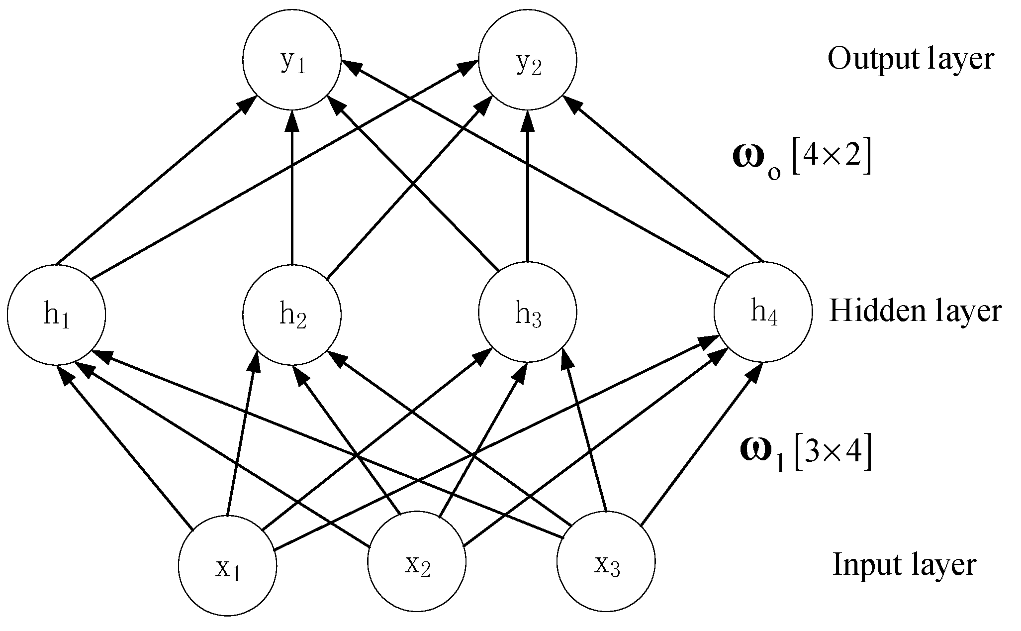
2.2. Deep Neural Network

A neural network generally consists of three layers: An input layer, a hidden layer, and an output layer. As shown in Figure 1, it is a simple neural network with three inputs and two outputs and four neurons in a single hidden layer. The neurons between layers are connected by weight $\omega$. The DNN contains multiple hidden layers, which has a significant improvement in the nonlinear fitting ability of the DNN compared with the single hidden layer. However, too many hidden layers are likely to cause over-fitting. The learning process of the network is the process of adjusting and determining the connection weights $\omega$ of each neuron through training samples.

In this paper, the LMBP algorithm is used to train DNN. Compared with the traditional back propagation (BP) algorithm, the LMBP algorithm has faster convergence speed and higher convergence reliability. It is more suitable for training the DNN and can also satisfy the requirements of real-time ultrashort-term prediction. Unlike the traditional BP algorithm, which uses a gradient descent, the LMBP algorithm is based on the Gauss-Newton method of the least squares solution and takes the square of error $\mathit{v}$ as the objective function.

$$E\left(\mathit{\omega }\right)={\mathit{v}}^{\mathrm{T}}\left(\mathit{\omega }\right)\mathit{v}\left(\mathit{\omega }\right).$$

(7)

The second-order Taylor expansion and derivation of the objective function of Equations (2)–(7) can obtain the change of weight $\mathit{\omega }$ as follows:

$$\Delta \mathit{\omega }=-{\left[{\nabla }^{2}E\left(\mathit{\omega }\right)\right]}^{-1}\nabla E\left(\mathit{\omega }\right).$$

(8)

where:

$$\{\begin{array}{l}\nabla E\left(\mathit{\omega }\right)=2{\mathit{J}}^{\mathrm{T}}\left(\mathit{\omega }\right)\mathit{v}\left(\mathit{\omega }\right)\\ {\nabla }^{2}E\left(\mathit{\omega }\right)=2{\mathit{J}}^{\mathrm{T}}\left(\mathit{\omega }\right)\mathit{J}\left(\mathit{\omega }\right)+2{\nabla }^2{\mathit{v}}^{\mathrm{T}}\left(\mathit{\omega }\right)\mathit{v}\left(\mathit{\omega }\right)\end{array}.$$

(9)

$\mathit{J}\left(\mathit{\omega }\right)$ is the Jacobian matrix of $\mathit{v}\left(\mathit{\omega }\right)$. If $\mathit{v}\left(\mathit{\omega }\right)$ consists of $a$ elements, $\mathit{J}\left(\mathit{\omega }\right)$ can be written as follows:

$$\mathit{J}\left(\mathit{\omega }\right)=\left[\begin{array}{cccc}\frac{\partial v_1}{\partial {\omega }_1}& \frac{\partial v_1}{\partial {\omega }_2}& \cdots & \frac{\partial v_1}{\partial {\omega }_a}\\ \frac{\partial v_2}{\partial {\omega }_1}& \frac{\partial v_2}{\partial {\omega }_2}& \cdots & \frac{\partial v_2}{\partial {\omega }_a}\\ ⋮& ⋮& \ddots & ⋮\\ \frac{\partial v_a}{\partial {\omega }_1}& \frac{\partial v_a}{\partial {\omega }_2}& \cdots & \frac{\partial v_a}{\partial {\omega }_a}\end{array}\right].$$

(10)

Since $2{\nabla }^2{\mathit{v}}^{\mathrm{T}}\left(\mathit{\omega }\right)\mathit{v}\left(\mathit{\omega }\right)$ is usually negligible, Formula (8) can be rewritten as follows:

$$\Delta \mathit{\omega }=-{\left[{\mathit{J}}^{\mathrm{T}}\left(\mathit{\omega }\right)\mathit{J}\left(\mathit{\omega }\right)\right]}^{-1}{\mathit{J}}^{\mathrm{T}}\left(\mathit{\omega }\right)\mathit{v}\left(\mathit{\omega }\right).$$

(11)

Considering that ${\mathit{J}}^{\mathrm{T}}\left(\mathit{\omega }\right)\mathit{J}\left(\mathit{\omega }\right)$ may be irreversible, Formula (11) is modified by adding the correction coefficient $\mu$, where $\mathit{I}$ is the unit matrix.

$$\Delta \mathit{\omega }=-{\left[{\mathit{J}}^{\mathrm{T}}\left(\mathit{\omega }\right)\mathit{J}\left(\mathit{\omega }\right)+\mu \mathit{I}\right]}^{-1}{\mathit{J}}^{\mathrm{T}}\left(\mathit{\omega }\right)\mathit{v}\left(\mathit{\omega }\right).$$

(12)

Similar to the BP algorithm, the modification of weight ${\mathit{\omega }}^{\left(k+1\right)}$ in the kth iteration is shown in Formula (13). $\Delta {\mathit{\omega }}^{\left(k\right)}$ can be obtained by Formula (12). When $E\left({\mathit{\omega }}^{\left(k+1\right)}\right)<\epsilon$, the algorithm has converged, where $\epsilon$ is the given error limit.

$${\mathit{\omega }}^{\left(k+1\right)}={\mathit{\omega }}^{\left(k\right)}+\Delta {\mathit{\omega }}^{\left(k\right)}.$$

(13)

The initial value of $\mu$ generally takes a small positive number such as 0.001. If the objective function $E\left({\mathit{\omega }}^{\left(k\right)}\right)$ becomes lower in the kth iteration, ${\mu }^{\left(k\right)}$ is divided by a factor $\theta$ as ${\mu }^{\left(k+1\right)}$ of the next iteration. If the objective function $E\left({\mathit{\omega }}^{\left(k\right)}\right)$ becomes higher in the kth iteration, the iteration will be restarted and multiply ${\mu }^{\left(k\right)}$ by the factor xxx as $\theta$ of this iteration. $\theta$ generally takes a number greater than 1, such as 4.

3. Ultrashort-Term Load Forecasting Model Based on Phase Space Reconstruction and Deep Neural Network

The traditional load fluctuation is mainly caused by user fluctuations in power usage. Although the electricity consumption of the user is uncertain, there are certain rules in general, and the fluctuation range is not large. For ultrashort-term prediction, linear extrapolation, time series prediction, and other methods can usually achieve the required accuracy. With the massive access of distributed energy sources such as PV power plants, the net load can be expressed by Formula (14). $p_t$ is the actual net load, $p^{\prime }$ is the user’s electricity load, and $p_t^{\mathrm{PV}}$ is the opposite number of PV power generation.

$$p_t=p_t^{\prime }+p_t^{\mathrm{PV}}.$$

(14)

Since the amount of PV power generation is as uncertain as the power load and different from the traditional power supply with a known power output, the PV power generation can be considered a load, which reduces the dispatching burden of the system. As a result, the uncertainty of load increases, and the range of fluctuation enlarges, even the situation of power reversal will occur at noon on sunny days. If the traditional forecasting method is also used, it will produce larger errors and cannot accurately predict the load.

Since the load is a non-linear time series with large fluctuations after the distributed energy access, it is difficult to directly predict. Therefore, the complex short-term prediction model may not satisfy the real-time requirements. In this paper, the phase space reconstruction is used to project the load time series into a time-varying and short-term regularity point in the high-dimensional phase space. Then, the non-linear fitting ability and fast convergence speed of LMBP DNN are used to fit and predict the locus of the points in the phase space to realize the ultrashort-term prediction of the load considering the distributed energy.

3.1. Modelling Steps of Prediction Model

For a series of net load time series $\mathit{p}=\left\{p_1,p_2\cdots p_N\right\}$ considering the PV power generation, the modelling, and forecasting steps of ultrashort-term forecasting model based on phase space reconstruction and DNN are as follows:

• Step 1: The load time series is linearly normalized to facilitate the training of DNN. The maximum and minimum values of the data are saved for the reverse normalization of the load forecasting value to restore the actual value.
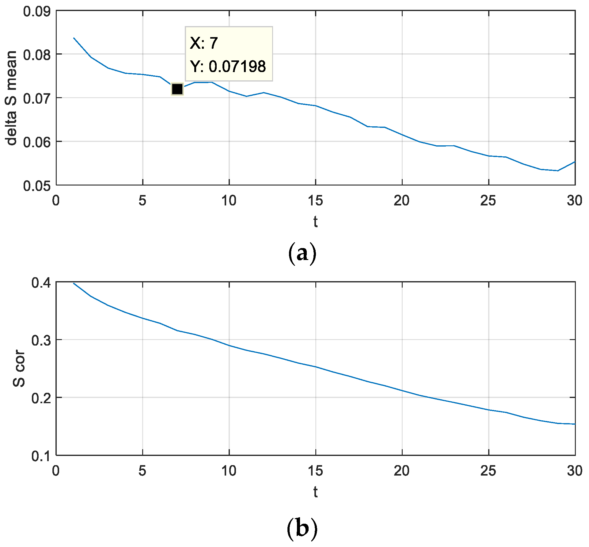
• Step 2: The C-C method is used to process the load time series, and the optimal embedded dimension m_opt and optimal delay t_opt of the time series are obtained.
• Step 3: The load time series are reconstructed according to the embedding dimension m and delay t obtained in Step 2. The phase space matrix of the reconstructed load time series is as follows. In Formula (15), $M=N-(m-1)t$.

  $$\left[\begin{array}{c}{\mathit{p}}_1\\ {\mathit{p}}_2\\ ⋮\\ {\mathit{p}}_M\end{array}\right]=\left[\begin{array}{cccc}{p}_1& p_{1+t}& \cdots & p_{1+(m-1)t}\\ p_2& p_{2+t}& \cdots & p_{2+(m-1)t}\\ ⋮& ⋮& \cdots & ⋮\\ p_M& p_{M+t}& \cdots & p_N\end{array}\right].$$

  (15)
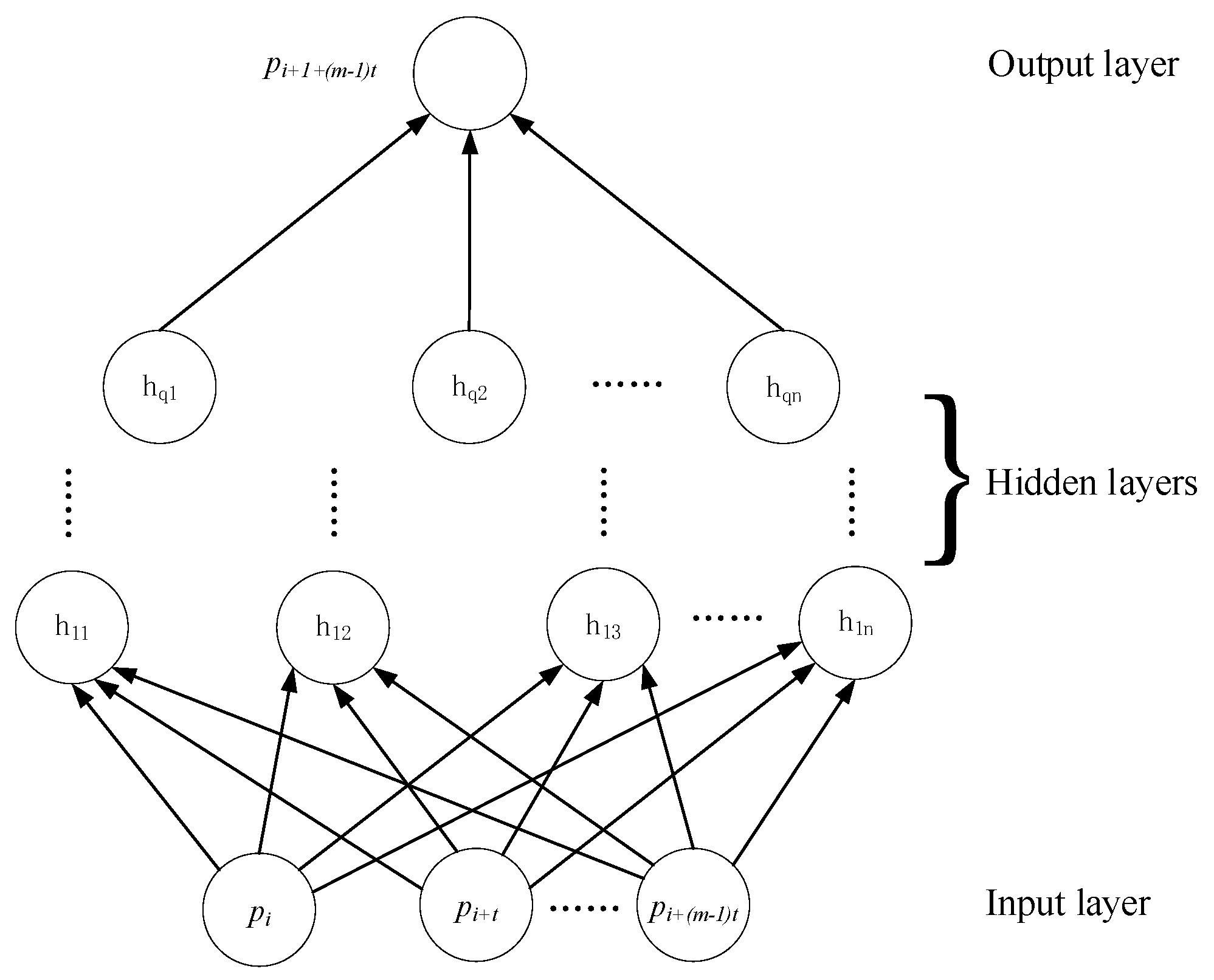
• Step 4: The p neural network is constructed, and the phase space matrix of load time series reconstructed in Step 3 is used as the training set to train the DNN. The trained DNN is used to predict the load value immediately after training.
• Step 5: Using the maximum and minimum values stored in Step 1, the load prediction values returned by the DNN are inverse-normalized to obtain the actual load prediction values.
• The model workflow chart is shown in Figure 2.

3.2. Determination of the Structure of Deep Neural Networks

The determination of the structure of the DNN is a link of the neural network hyper-parameter adjustment. An unreasonable structure can make the prediction results of the DNN seriously deviate. If the training time is too long, the work is half the effort. The specific method of determination is as follows:

• Input layer

If the DNN is directly trained using the original load data, the determination of the number of neurons in the input layer can be very difficult and requires a lot of debugging to obtain the optimal value. Moreover, when the training set data changes, previous optimal values may no longer be applicable, and the structure of the input layer must be re-debugged. In this model, the input data of the DNN is the phase space reconstructed matrix. Therefore, the number of neurons in the input layer is directly determined by the embedding dimension m obtained by the C-C method without artificial designation or after debugging to select the optimal value.

• Hidden layer

The number of hidden layers can be heuristically determined. When there are few hidden layers, the model will have an under-fitting and cause a large deviation in the predicted value. Conversely, too many hidden layers can cause a model overfitting. The number of hidden layers can be gradually increased during the trial until the predicted value shows a significant over-fitting. Then, we gradually reduce the number of hidden layers so that the predicted value and true value of the model are as similar as possible on the verification set to determine the optimal number of hidden layers. The number of neurons in each hidden layer can be taken as 75% of the number of neurons in the upper layer but generally more than the number of neurons in the output layer. The activation function of the hidden layer neurons usually uses the tanh function and rectified linear unit (ReLU) function. The tanh function is used in this paper.

• Output Layer

The prediction model in this paper adopts the one-step prediction. Only the load value at the next moment is predicted at a given time. Therefore, after the load time series is projected to the moving point in the phase space, the model must output the position vector of the point in the phase space of the next time. In fact, if the input of the model is ${\mathit{p}}_i\left(1\le i\le M\right)$ in the phase space reconstruction matrix of Formula (15), only $p_{i+1+(m-1)t}$ is unknown in position vector ${\mathit{p}}_{i+1}$ at the next moment. Therefore, the output layer must only output the predicted value of load ${\widehat{p}}_{i+1+(m-1)t}$. If $i+1>M$, the phase space reconstruction matrix of Formula (15) must be extended downward, and ${\mathit{p}}_{i+1}$ is added as a new line. The expression of ${\mathit{p}}_{i+1}$ is shown in Formula (16), where $p_{i+1+(m-1)t}$ is the true value of the newly measured load.

$${\mathit{p}}_{i+1}=\left[\begin{array}{cccc}{p}_{i+1}& p_{i+1+t}& \cdots & p_{i+1+(m-1)t}\end{array}\right]$$

(16)

${\mathit{p}}_{i+1}$ is used as the input of the model to obtain the predicted value of $p_{i+2+(m-1)t}$; then, the matrix is augmented, and the predicted value of $p_{i+3+(m-1)t}$ is obtained, and the process continues until the end of the prediction. The activation function of the output layer is a linear function. The DNN structure is shown in Figure 3.

DNN can be widely used in different areas. In addition to load forecasting, DNN can also solve the problems including image processing, speech recognition, and fault diagnosis. The training method and network structure are basically the same. The difference is the training data. For the prediction of time series load data, the output layer is the actual load data. For the image processing and fault diagnosis, the output layer is the data label. The structure of DNN is basically the same as the traditional ANN, but the training method is improved which make it have better performance.

4. Analysis of Prediction Results

To verify the validity of the model, the proposed model was validated in MATLAB R2018a. In this paper, the net load data of the upper bus of a city’s PV substation in the first 15 days of May 2017 were used. The sampling interval of the net load data is 5 min, and the installed capacity of the distributed PV power station is approximately 50 MW. The data from 1–11 May were selected as the training set to model the prediction model, and the parameters of the model were adjusted by cross-validation. The data from 12–15 May were selected as the samples of the prediction test, where 12 May was sunny, and 13–15 May were cloudy.

4.1. Result of the Phase Space Reconstruction by the C-C Method

The net load data from 1–11 May were processed by the C-C method. The corresponding statistics of $\overline{\Delta S}\left(t\right)$ and $S_{cor}\left(t\right)$ are shown in Figure 4. The first extremum point of $\overline{\Delta S}\left(t\right)$ was $t=7$. $S_{cor}\left(t\right)$ had no obvious minimum point, and the optimal embedded window $t_{\omega }$ was not obtained. According to the BDS statistics, when $N>3000$, $m\in \left\{2,3,4,5\right\}$, so the maximum value of m could only take 5. According to Formula (6), the final optimal embedding dimension m_opt = 5 and optimal delay t_opt = 7 were obtained.

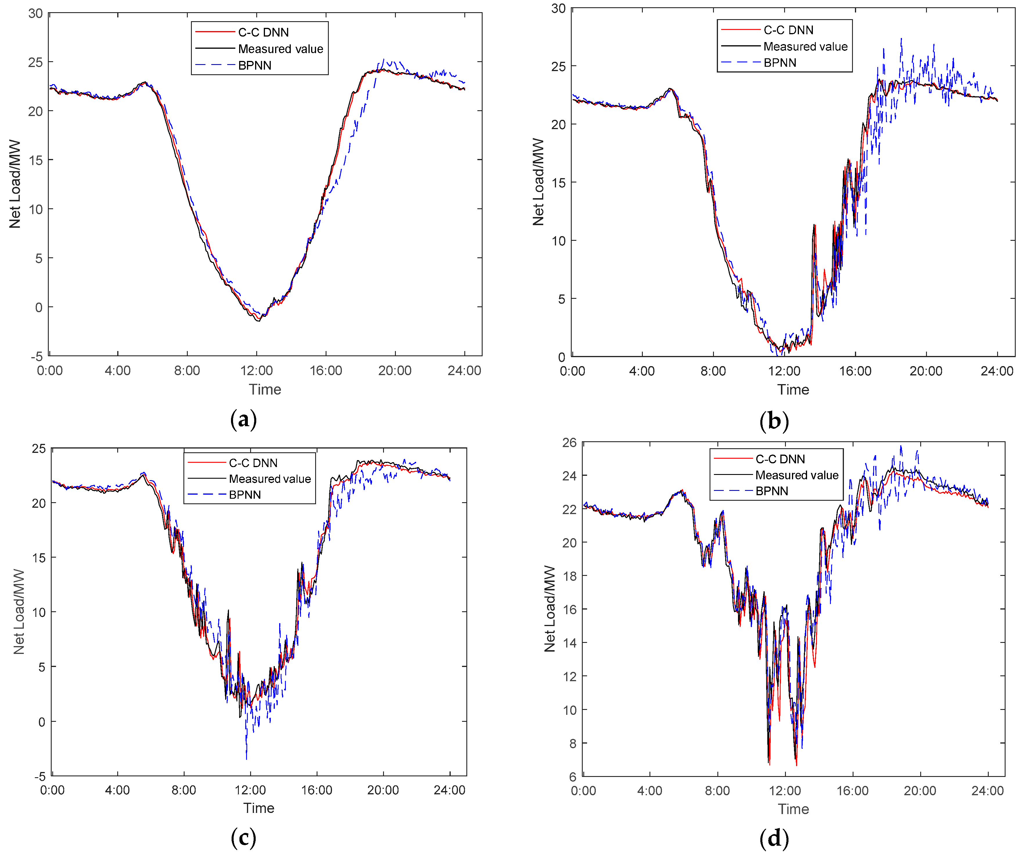
4.2. Prediction Results of the Deep Neural Network

Since the embedding dimension is m = 5 as determined by the C-C method, there were five input neurons in the DNN. The cross-validation shows that when the number of layers in the hidden layer was 5, the predicted value showed a significant over-fitting. Therefore, the number of layers of the hidden layer was taken as 4, and the neurons of each hidden layer were taken as 5, 4, 3, and 2. The DNN used the single-step prediction and only predicted the next 5 min load value at a time. The predicted result is shown in Figure 5. The black solid line is the actual net load, the red solid line is the ultrashort-term prediction value based on the phase space reconstruction and DNN, and the blue dotted line is the ultrashort-term prediction value based on the traditional BP neural network.

In Figure 5, at approximately 12:00 noon on a clear day (12th), a negative power was present in the payload due to an increase in the amount of PV power generation. The prediction results based on the phase space reconstruction and DNN were closer to the actual net load value, which was obviously better than the prediction results using the traditional BP neural network.

On cloudy days (13–15 May), when the net load sharply fluctuated due to the fluctuation of the PV output, although the actual net load value was stable, the predicted value of the traditional BP neural network still had large fluctuations, which resulted in a large deviation. However, the prediction results based on the phase space and DNN did not strongly deviate and basically conformed to the actual trend of the net load.

To accurately evaluate the accuracy of the model prediction and the accuracy of prediction, the mean absolute percentage error (MAPE) and root mean square error (RMSE) were used as evaluation indicators. In Formulas (17) and (18), n is the number of predicted samples, $p_i$ is the actual value of the net load at time i, and ${\widehat{p}}_i$ is the predicted value of the net load at time i.

$$\mathrm{MAPE}=\frac{1}{n}{\displaystyle \sum _{i=1}^n}\left|\frac{p_i-{\widehat{p}}_i}{p_i}\right|\times 100\%$$

(17)

$$\mathrm{RMSE}=\sqrt{\frac{1}{n}{\displaystyle \sum _{i=1}^n{\left(p_i-{\widehat{p}}_i\right)}^2}}$$

(18)

The prediction accuracy is shown in

Table 1. Prediction accuracy of different models.

Date	MAPE (%)		RMSE
	C-C DNN	BPNN	C-C DNN	BPNN
12 May (Sunny)	8.8838	18.3725	0.8973	1.3327
13 May (Cloudy)	9.9978	17.6827	1.3970	1.8242
14 May (Cloudy)	15.4156	17.6415	1.1193	1.3648
15 May (Sunny)	4.0648	4.6388	1.0972	1.1916

. Compared with the prediction model based on the traditional BP neural network, the forecasting scheme proposed in this paper improved the accuracy of net load forecasting under different weather conditions. On a cloudy day (15 May), the power of PV power generation was very small. The accuracy of the prediction model based on the phase space reconstruction and the deep neural network was basically identical to that based on the traditional BP neural network. However, on a sunny day (12 May), the PV power was relatively high, and the difference of MAPE between the two models was nearly 10%. The predictive models based on the phase space reconstruction and DNN still had higher prediction accuracy even in the case of large distributed PV power access and large power fluctuation.

5. Conclusions

• A large amount of access to the distributed PV power generation results in the increasing fluctuation of the net load power, which challenges the ultrashort-term load forecasting. Considering this phenomenon and the characteristics of ultrashort-term load forecasting, this paper presents a model of ultrashort-term load forecasting based on the phase space reconstruction and DNN. Based on the phase space reconstruction, the time series is projected into a moving point in the phase space, and the DNN is subsequently used to fit the trajectory to realize the load forecasting.
• The prediction of the actual load data and a comparison experiment with the BP neural network prediction model have verified that the proposed model has higher prediction accuracy even in the case of large distributed PV power fluctuations and different weather conditions. In particular, when there is a large amount of PV power access and high penetration, there is also an ideal predictive performance.

References

1. Li, L.L.; Sun, J.; Wang, C.H.; Zhou, Y.T.; Lin, K.P. Enhanced Gaussian process mixture model for short-term electric load forecasting. Inf. Sci. 2019, 477, 386–398. [Google Scholar] [CrossRef]
2. Sun, W.; Zhang, C.C. A Hybrid BA-ELM Model Based on Factor Analysis and Similar-Day Approach for Short-Term Load Forecasting. Energies 2018, 11, 1282. [Google Scholar] [CrossRef]
3. Barman, M.; Choudhury, N.B.D.; Sutradhar, S. A regional hybrid GOA-SVM model based on similar day approach for short-term load forecasting in Assam, India. Energy 2018, 145, 710–720. [Google Scholar] [CrossRef]
4. Zhang, J.L.; Wei, Y.M.; Li, D.Z.; Tan, Z.F.; Zhou, J.H. Short term electricity load forecasting using a hybrid model. Energy 2018, 158, 774–781. [Google Scholar] [CrossRef]
5. Li, Y.Y.; Han, D.; Yan, Z. Long-term system load forecasting based on data-driven linear clustering method. J. Mod. Power Syst. Clean Energy 2018, 6, 306–316. [Google Scholar] [CrossRef]
6. Bennett, C.J.; Stewart, R.A.; Lu, J.W. Forecasting low voltage distribution network demand profiles using a pattern recognition based expert system. Energy 2014, 67, 200–212. [Google Scholar] [CrossRef] [Green Version]
7. Kazemi, S.M.R.; Hoseini, M.M.S.; Abbasian-Naghneh, S.; Rahmati, S.H.A. An evolutionary-based adaptive neuro-fuzzy inference system for intelligent short-term load forecasting. Int. Trans. Oper. Res. 2014, 21, 311–326. [Google Scholar] [CrossRef]
8. Ahmad, T.; Chen, H.X. Nonlinear autoregressive and random forest approaches to forecasting electricity load for utility energy management systems. Sustain. Cities Soc. 2019, 45, 460–473. [Google Scholar] [CrossRef]
9. Massidda, L.; Marrocu, M. Smart Meter Forecasting from One Minute to One Year Horizons. Energies 2018, 11, 3520. [Google Scholar] [CrossRef]
10. Alamaniotis, M.; Ikonomopoulos, A.; Tsoukalas, L.H. Evolutionary Multiobjective Optimization of Kernel-Based Very-Short-Term Load Forecasting. IEEE Trans. Power Syst. 2012, 27, 1477–1484. [Google Scholar] [CrossRef]
11. Alamaniotis, M.; Bargiotas, D.; Tsoukalas, L.H. Towards smart energy systems: Application of kernel machine regression for medium term electricity load forecasting. Springerplus 2016, 5, 58. [Google Scholar] [CrossRef] [PubMed]
12. Amjady, N. Evolutionary Multiobjective Short-term bus load forecasting of power systems by a new hybrid method. IEEE Trans. Power Syst. 2007, 22, 333–341. [Google Scholar] [CrossRef]
13. Hossen, T.; Plathottam, S.J.; Angamuthu, R.K.; Ranganathan, P.; Salehfar, H. Short-Term Load Forecasting Using Deep Neural Networks (DNN). In Proceedings of the 2017 North American Power Symposium (NAPS), Morgantown, WV, USA, 17–19 September 2017. [Google Scholar]
14. Chen, Y.; Luh, P.B.; Guan, C.; Zhao, Y.; Michel, L.D.; Coolbeth, M.A.; Friedland, P.B.; Rourke, S.J. Short-Term Load Forecasting: Similar Day-Based Wavelet Neural Networks. IEEE Trans. Power Syst. 2010, 25, 322–330. [Google Scholar] [CrossRef]
15. Moon, J.; Kim, Y.; Son, M.; Hwang, E. Hybrid Short-Term Load Forecasting Scheme Using Random Forest and Multilayer Perceptron. Energies 2018, 11, 3283. [Google Scholar] [CrossRef]
16. Nazar, M.S.; Fard, A.E.; Heidari, A.; Shafie-Khah, M.; Catalao, J.P.S. Hybrid model using three-stage algorithm for simultaneous load and price forecasting. Electr. Power Syst. Res. 2018, 165, 214–228. [Google Scholar] [CrossRef]
17. Zhang, B.; Liu, W.; Li, S.T.; Wang, W.G.; Zou, H.; Dou, Z.H. Short-term load forecasting based on wavelet neural network with adaptive mutation bat optimization algorithm. IEEJ Trans. Electr. Electron. Eng. 2019, 14, 376–382. [Google Scholar] [CrossRef]
18. Liang, Y.; Niu, D.X.; Hong, W.C. Short term load forecasting based on feature extraction and improved general regression neural network model. Energy 2019, 166, 653–663. [Google Scholar] [CrossRef]
19. Dai, S.Y.; Niu, D.X.; Li, Y. Daily Peak Load Forecasting Based on Complete Ensemble Empirical Mode Decomposition with Adaptive Noise and Support Vector Machine Optimized by Modified Grey Wolf Optimization Algorithm. Energies 2018, 11, 163. [Google Scholar] [CrossRef]
20. Heymann, F.; Silva, J.; Miranda, V.; Melo, J.; Soares, F.J.; Padilha-Feltrin, A. Distribution network planning considering technology diffusion dynamics and spatial net-load behavior. Int. J. Electr. Power Energy Syst. 2019, 106, 254–265. [Google Scholar] [CrossRef]
21. Elghitani, F.; El-Saadany, E. Smoothing Net Load Demand Variations Using Residential Demand Management. IEEE Trans. Ind. Inform. 2019, 15, 390–398. [Google Scholar] [CrossRef]
22. Kuppannagari, S.R.; Kannan, R.; Prasanna, V.K. Optimal Discrete Net-Load Balancing in Smart Grids with High PV Penetration. ACM Trans. Sens. Netw. 2018, 14, 24. [Google Scholar] [CrossRef]
23. Zhou, X.; Zi, X.H.; Liang, L.Q.; Fan, Z.B.; Yan, J.W.; Pan, D.M. Forecasting performance comparison of two hybrid machine learning models for cooling load of a large-scale commercial building. J. Build. Eng. 2018, 21, 64–73. [Google Scholar] [CrossRef]
24. Kong, W.C.; Dong, Z.Y.; Jia, Y.W.; Hill, D.J.; Xu, Y.; Zhang, Y. Short-Term Residential Load Forecasting Based on LSTM Recurrent Neural Network. IEEE Trans. Smart Grid 2019, 10, 841–851. [Google Scholar] [CrossRef]
25. Kim, H.S.; Eykholt, R.; Salas, J.D. Nonlinear dynamics, delay times, and embedding windows. Physica D 1999, 127, 48–60. [Google Scholar] [CrossRef]
Figure 1. Single-hidden-layer neural network.
Applsci 09 01487 g001
Figure 2. Forecasting model flow chart.
Applsci 09 01487 g002
Figure 3. Deep neural network structure.
Applsci 09 01487 g003
Figure 4. Curves of Δ S ¯ ( t ) and S c o r ( t ) . (a) Curve of statistic Δ S ¯ ( t ) ; (b) Curve of statistic S c o r ( t ) .
Applsci 09 01487 g004
Figure 5. Load forecasting results based on different models: (a) 12 May; (b) 13 May; (c) 14 May; (d) 15 May.
Applsci 09 01487 g005