A Tabu List-Based Algorithm for Capacitated Multilevel Lot-Sizing with Alternate Bills of Materials and Co-Production Environments

Featured Application

Small and medium enterprises with complex production systems, involving multi-level product structures and co-production configurations, would use the proposed algorithm for improving their production planning and lot-sizing decisions.

Abstract

The definition of lot sizes represents one of the most important decisions in production planning. Lot-sizing turns into an increasingly complex set of decisions that requires efficient solution approaches, in response to the time-consuming exact methods (LP, MIP). This paper aims to propose a Tabu list-based algorithm (TLBA) as an alternative to the Generic Materials and Operations Planning (GMOP) model. The algorithm considers a multi-level, multi-item planning structure. It is initialized using a lot-for-lot (LxL) method and candidate solutions are evaluated through an iterative Material Requirements Planning (MRP) procedure. Three different sizes of test instances are defined and better results are obtained in the large and medium-size problems, with minimum average gaps close to 10.5%.

1. Introduction

The definition of lot sizes represents one of the most important decisions in production planning. Lot-sizing models aim to guarantee the fulfillment of the demand requirements, establishing a balance between holding and setup costs. Complex assembly systems usually require wide and robust product structures, which may involve the use of alternate bills of materials and co-production settings. In these cases, the complexity of lot sizing decisions increases along with flexibility. Depending on the problem size and the number of considered constraints, the use of exact solution models can be inefficient in terms of computational times, especially for operational planning purposes [1,2].

Exact solution approaches have been widely used for the NP-hard Capacitated Lot Sizing Problem (CLSP), including cut-generation [3] and redefinition techniques [4], supported by mathematical approaches as Branch and Bound, Lagrangian Relaxation, and Wagner-Within. In the case of multi-level CLSP, the use of linear programming (LP) methods showed good results [5].

On the other hand, the use of heuristic and meta-heuristic methods for solving lot-sizing problems has become increasingly frequent and implementations have flooded the scientific literature [2,6,7,8,9]. The advantages of these kinds of approximate procedures include reduced computational times, the ability to solve larger problems, higher flexibility, high-quality solutions, and reduced implementation costs (e.g., compared with commercial software licenses [10]).

Among the different heuristic approaches, local and guided-search algorithms, such as the Tabu Search (TS), have demonstrated efficiency in a variety of lot-sizing problems, especially with multi-product and multi-level planning structures [11,12,13]. Most implementations take initial solutions from constructive algorithms, which are later improved with iterative small modifications (called moves). The search is guided by long-term and short-term memory structures within intensification and diversification phases [9,14,15,16].

The Generic Materials and Operations Planning model (GMOP) is one of the most recent exact models for solving lot-sizing problems that considers alternative bills of materials, multi-level structures, multi-site production/packaging, and co-production settings. This model was proposed in 2011 [17,18] as a robust mixed integer programming (MIP) problem. Since 2013 [19,20], the functioning of GMOP has been improved with the implementation of mathematical relaxation methods and its efficiency in practical applications has been demonstrated (e.g., in the automotive sector) [21,22,23].

Developing heuristic approaches for solving this problem has been suggested as a research opportunity since 2012 [24,25], but these kinds of procedures have not been extensively explored [26]. Proposing alternative solution methods and data structures represents a contribution not only to further GMOP studies, but also to the wider research field of multi-level lot-sizing problems, employing alternative product structures instead of the generalized Gozinto structure.

The aim of this article is to propose an alternative heuristic algorithm for the GMOP, using the short-term memory principles of TS. The main considerations include: Capacity constraints, a multi-product/multi-level structure, a co-production environment, and the existence of alternate bills of materials for final products [27,28].

This paper is organized as follows. Section 2 shows the GMOP generalities. Section 3 shows a brief introduction to TS algorithms. Section 4 exposes the methodological framework and a functioning overview of the proposed algorithm. The obtained results and their discussion are shown, respectively, in Section 5 and Section 6. Finally, conclusions and further research opportunities are highlighted in Section 7.

2. The Generic Materials and Operational Planning Model (GMOP)

The Generic Materials and Operational Planning model was proposed by Garcia Sabater et al. [19] and Maheut et al. [18], as an alternative for modeling the existing relations between the processes and the materials needed for the elaboration of a product.

Unlike the Gozinto representation (where the priority falls on the final product and its components), this lot-sizing model focuses on the planning of operations (strokes) to be made for the manufacture, purchase, or transportation of a certain product or a group of products.

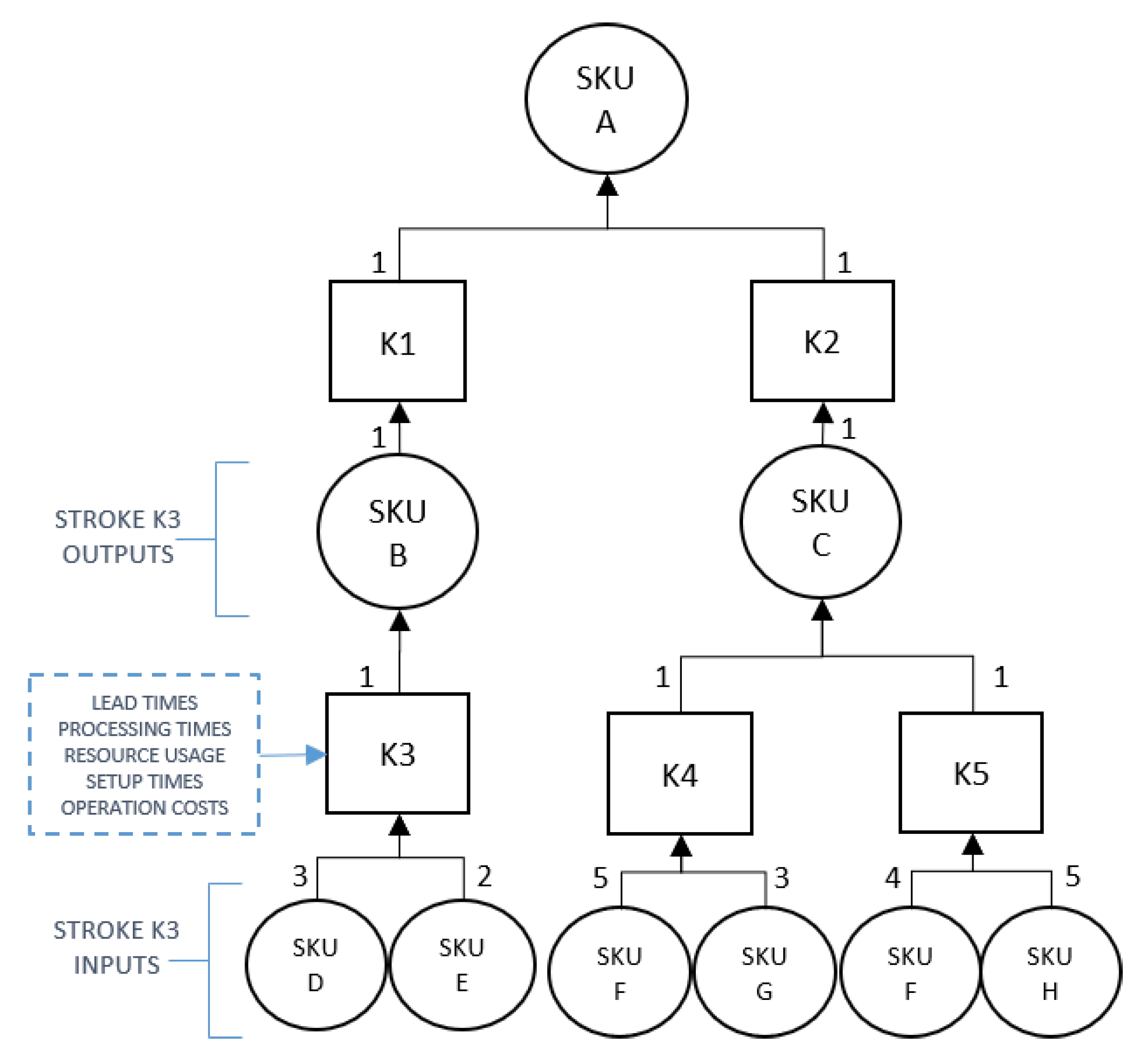
A stroke is defined as any activity or operation that allows for the transformation of a set of products or Stock Keeping Units (SKUs) into another set of SKUs, using or immobilizing a certain amount of resources. As shown in Figure 1, a Stroke can contain the following attributes [19]:

• Outputs (Stroke Outputs): The product or set of products obtained from the stroke execution, as shown in

  Table 1. Stroke outputs matrix, according to Figure 1.

  ${\mathit{SO}}_{\mathit{i},\mathit{k}}$	k1	k2	k3	k4	k5
  SKU A	1	1	0	0	0
  SKU B	0	0	1	0	0
  SKU C	0	0	0	1	1
  SKU D	0	0	0	0	0
  SKU E	0	0	0	0	0
  SKU F	0	0	0	0	0
  SKU G	0	0	0	0	0
  SKU H	0	0	0	0	0

  .
• Inputs (Stroke Inputs): The product or set of products consumed at the execution of the stroke, as shown in

  Table 2. Stroke inputs matrix, according to Figure 1.

  ${\mathit{SI}}_{\mathit{i},\mathit{k}}$	k1	k2	k3	k4	k5
  SKU A	0	0	0	0	0
  SKU B	1	0	0	0	0
  SKU C	0	1	0	0	0
  SKU D	0	0	3	0	0
  SKU E	0	0	2	0	0
  SKU F	0	0	0	5	4
  SKU G	0	0	0	3	0
  SKU H	0	0	0	0	5

  .
• Lead times
• Operation times and costs
• Set-up times and costs
• Resource usage: Resources can be, for example, machinery, workforce, and so on.

The GMOP model can easily include capacity constraints, as well as direct, inverse, and alternate bill of materials, multi-site production, resource requirements, by-products, transportation modes, and packaging processes [19].

The problem is presented as a mixed integer programming model, whose parameters and variables are shown in

Table 3. Parameters and decision variables for the GMOP model [19].

Symbol	Description
i	Index set of products (includes product, packaging, and site)
t	Index set of planning periods
r	Index set of resources
k	Index set of strokes
$D_{i,t}$	Demand of product i for period t
$hi,t$	Cost of storing a unit of product i in period t
$C{O}_{k,t}$	Cost of stroke k in period t
$C{S}_{k,t}$	Cost of the setup of stroke k in period t
$C{B}_{i,t}$	Cost of purchasing product i in period t
$S{O}_{i,k}$	Number of units i that generates a stroke k
$S{I}_{i,k}$	Number of units i that stroke k consumes
$L{T}_k$	Lead time of stroke k
$KA{P}_{r,t}$	Capacity availability of resource r in period t (in time units)
M	A sufficiently large number
$T{O}_{k,r}$	Capacity of the resource r required for performing one unit of stroke k (in time units)
$T{S}_{k,r}$	Capacity required of resource r for setup of stroke k (in time units)
$z_{k,t}$	Amount of strokes k to be performed in period t
${\delta }_{k,t}$	=1 if stroke k is performed in period t (and 0 otherwise)
$w_{i,t}$	Purchase quantity for product i in period t
$X_{i,t}$	Stock level of product i on hand at the end of period t
Z	Total Planning Cost

. The objective function (1) aims to minimize the total planning cost Z, which includes storage, operation, and set up costs generated by the execution of strokes.

Equation (2) represents the inventory constraint. It considers the stock levels from the previous period, demand requirements, purchased items, and the quantities generated and consumed by the strokes in every time period.

Equation (3) ensures the inclusion of a setup cost when a stroke is used: If $z_{k,t}$ is larger than zero, then ${\delta }_{k,t}$ must be 1 in order to satisfy the constraint.

Equation (4) is a capacity constraint that limits the use of resources by considering both setup and operations times.

Finally, Equations (5)–(8) define the range and domain of the decision variables.

$$Z=Min\sum _t\sum _i(h_{i,t}\ast X_{i,t})+\sum _t\sum _k(C{S}_{k,t}\ast {\delta }_{k,t}+C{O}_{k,t}\ast z_{k,t})+\sum _t\sum _i(C{B}_{i,t}\ast w_{i,t})$$

(1)

$$X_{i,t}=X_{i,t-1}-D_{i,t}+w_{i,t}-\sum _k(S{I}_{i,k}\ast z_{k,t})+\sum _k(S{O}_{i,k}\ast z_{k,t-L{T}_k})\forall (i,t)$$

(2)

$$z_{k,t}-M\ast {\delta }_{k,t}\le 0\forall (k,t)$$

(3)

$$\sum _k(T{S}_{k,r}\ast {\delta }_{k,t})+\sum _k(T{O}_{k,r}\ast z_{k,t})\le KA{P}_{r,t}\forall (r,t)$$

(4)

$$X_{i,t}\ge 0$$

(5)

$$w_{i,t}\ge 0$$

(6)

$$z_{k,t}\in {\mathbb{Z}}^{+}$$

(7)

$${\delta }_{k,t}\in \left\{0,1\right\}.$$

(8)

3. Tabu Search Algorithms

The Tabu Search (TS) method is a metaheuristic method proposed by Glover in 1989 [29] and 1993 [30]. It is an iterative procedure which explores a set of problem solutions, making moves from one solution x to another solution $x^{\prime }$ inside a neighborhood $V\left(x\right)$. Moves aim to find optimal or near-optimal solutions, evaluating some objective function that is to be minimized.

TS involves adaptive memory principles, the creation of constrained search spaces, and the utilization of short-term and long-term learning mechanisms [31].

The Tabu list is the main short-term memory mechanism and keeps a record of the most recently adopted moves, keeping the algorithm from re-evaluating previously-considered solutions and getting stuck in local optima. The algorithm starts with an initial solution $Z_0$ as the current solution S. Moves allow the algorithm to make changes to the solution array, generating candidate solutions $S_c$. These changes can be done using an insertion, mutation, combination, or by crossing strategies.

A set V is generated with $N_s$ candidate solutions. After evaluation, only the best solution per iteration is adopted ($S\leftarrow S_c$) and the moves ($S_k$ to $S_c$) and ($S_c$ to $S_k$) are registered in the Tabu list, being forbidden for a specific number of iterations (the so-called Tabu tenure).

The algorithm stops when a completion criterion is fulfilled. The most frequent finalization conditions include a maximum number of iterations, a minimum value for the objective function, or a specific number of iterations without substantial improvements.

TS also allows for the implementation of aspiration, diversification, and intensification mechanisms. Aspiration criteria allow the algorithm to improve the solution by considering moves included in the Tabu list. Intensification mechanisms are short-term or long-term memory structures that allow a deep exploration of promising search spaces. Finally, diversification strategies guide the search towards poorly-explored search spaces [32].

TS algorithms have been implemented in a variety of lot-sizing and scheduling problems. This approach frequently offers high-quality solutions and has been able to outperform other heuristics and relaxation methods [12,33,34,35]. One of the main motivations for adopting a TS approach lies in the advantages of local search, especially its efficiency for managing hard constraints in large scale problems [36]. TS principles are especially useful when reducing search neighborhoods and guiding the search into feasible solutions.

The reference [9] shows one of the first TS implementations for a multi-level lot-sizing problem. The authors compared the performance between a pure Linear Programming (LP) method and two LP-based heuristics (LP combined with Simulated Annealing (SA) and TS) when solving a multi-level capacitated lot-sizing problem (MCLSP) in an assembly production system with bottleneck constraints. An initial solution was obtained with a modified greedy algorithm and the search was guided according to non-restricted moves with higher improvements in the objective function. No diversification, intensification, or aspiration mechanisms were specified. The results showed better performance in the LP-based approaches.

In [15], two different heuristic methods were proposed to solve a capacitated multi-level lot-sizing and scheduling problem for a multiple-item, single machine system. The first method was based on a “randomized regrets” heuristic, and the second was a TS-based heuristic. A Gozinto product structure was represented using a disjunctive arcs method, and moves were performed according to the existence of adjacent nodes with larger improvements in the objective function. The computational results were similar for both heuristics and the inclusion of multiple resources, setup times, and back-orders were proposed as future work opportunities.

Other well-known heuristic approaches, such as SA and Genetic Algorithms (GA), were tested and compared with TS in [12]. The obtained results showed that TS outperformed the SA and GA methods, especially when the problem involved confirmed order demand.

TS is usually combined with other methods in order to improve results. A hybrid algorithm TS–SA was proposed in [14] for solving a multi-level lot-sizing problem with general product structures. TS mechanisms were used to guide the search with the help of SA components. The results demonstrated that the inclusion of the TS method led to an improvement in cost performance, when compared with CPLEX–LP solutions.

In the case of single-level lot-sizing problems, TS has been tested within a wide variety of configurations and constraints: [37] showed a capacitated, single-item problem with dynamic demand. The multi-item variation for this problem was shown in [38].

In [39], the problem defined was multi-item with setup carry-over. The TS approach included dynamic Tabu lists and penalty constraints.

A dynamic lot-sizing problem with product returns and re-manufacturing constraints was presented in [35]. The initial solutions were generated using a blockchain-based algorithm and the TS algorithm was able to obtain satisfactory results in at least 96% of test instances.

4. Methods

4.1. Algorithm Overview

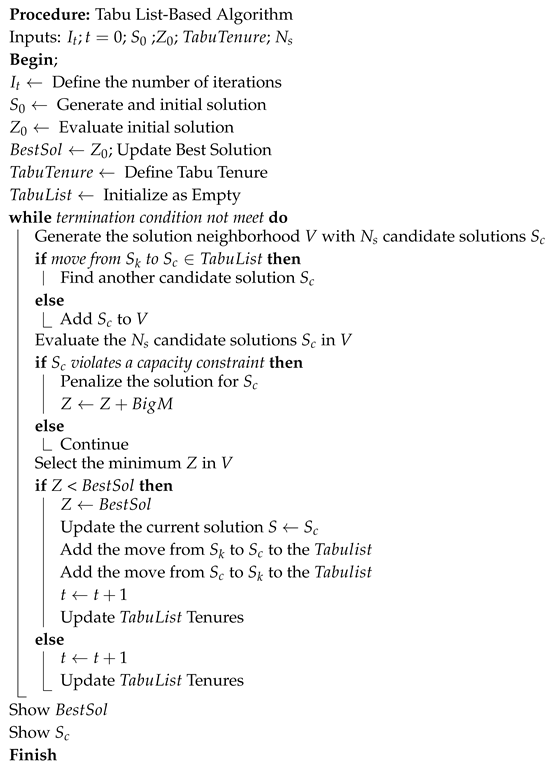
The proposed algorithm is an approximation to a TS method [29,40]. An outline of the Tabu list-based algorithm (TLBA) is shown in Algorithm 1.

Algorithm 1: Tabu List-based algorithm outline

4.2. Solution Array

The solution array $S_i$ contains the selected strokes for producing every SKU. Given the presence of alternate bills of materials, and that each stroke has different settings for inputs, outputs, and resource usage, it is necessary to decide which stroke is more efficient in producing each product, minimizing the total planning cost.

4.3. Search Neighborhood

The search neighborhood was composed by the set of solutions resulting from all possible stroke selections for each SKU. These possible selections were listed in the alternative stroke matrix $Al{t}_{i,k}$. The $Al{t}_{i,k}$ matrix is built from the output matrix $S{O}_{i,k}$ and contains a list of the strokes that can produce each SKU. If a SKU can be produced by more than one stroke, it can be said that this SKU has more than one bill of materials. At the same time, if a stroke has more than one output, we are facing a case of co-production.

4.4. Moves

For each iteration, a set V is built using $N_s$ neighbor solutions. A short-term diversification phase is used, and candidate solutions are obtained from the change of one random position (SKU) in $S_i$. When a random position is selected, an alternative stroke from $Al{t}_{i,k}$ is assigned. This move is only made for those SKUs that have at least one alternative stroke and a single change is made for each new generated $N_s$.

4.5. Evaluation Procedure

As shown in (1), the total planning cost included setups, operation, and holding costs, resulting from stroke utilization in each period. The total stroke requirements per period were calculated through a Material Requirement Planning (MRP) strategy, with a lot-for-lot policy [41] in every level of the product structures. When obtaining an initial solution, one important consideration for the evaluation procedure was the assumption that a product i is only produced using the first alternative stroke listed in $Al{t}_{i,k}$.

4.6. The Tabu List

The Tabu list is represented by a 3-dimensional data structure ${TabuList}_{k1,k2,i}$, which records the moves made from the current solution $S_i$ to the best solution $BestSol$ obtained in each iteration. For each $SKU\left(i\right)$, there is a square matrix of order k (total number of strokes), where $k1$ is the initial stroke and $k2$ is the final stroke in every move. The Tabu list contains, by default, a $BigM$ number in the positions of the main diagonal. This prevents the algorithm from making moves using the same stroke. As soon as a move enters the Tabu list, it is assigned with the Tabu tenure (this is the number of iterations that it will be included in the Tabu list). The opposite move is included as well. The number of forbidden moves in the Tabu list is equivalent to twice the selected Tabu tenure. The oldest moves will come out first and the most recent moves will come out later.

4.7. Completion Criteria

The algorithm stops with the fulfillment of a maximum number of iterations $It$.

5. Results

5.1. Test Instances

Table 4. Parameter settings for randomly-generated test cases [28].

Parameter	Value
i	50, 100, or 200 SKU
$i\ast$	15, 30, or 60 final products
t	25, 50, or 75 planning periods
r	5, 10, or 20 resources
k	50, 100, or 200 strokes
$D_{i,t}$	Uniform [1000, 2000]
$h_{i,t}$	Uniform [10, 20]
$C{O}_{k,t}$	Uniform [5, 8]
$C{S}_{k,t}$	Uniform [5, 10]
$S{O}_{i,k}$	Uniform [35, 50]
$S{I}_{i,k}$	Uniform [4, 8]
$L{T}_k$	Uniform [1, 2]
$KA{P}_{r,t}$	Uniform [2000, 6000]
	Uniform [4000, 8000]
	Uniform [12,000, 14,000]
$T{O}_{k,r}$	Uniform [2, 5]
$T{S}_{k,r}$	Uniform [5, 10]

shows the parameters used for the definition of the randomly-generated test instances (Based on the methodology in [12,14] and the values defined in [23]).

Nine groups of test instances were generated, according to three different sizes: Small (TI1–TI3), medium (TI4–TI6), and large (TI7–TI9).

Every instance group received an identification code, according to its parameters. For example, the test instance showed in Figure 2 represents a problem with 50 SKU, 15 final products, a planning horizon of 25 periods, 10 resources, and 50 strokes.

The generated test instances groups are listed below:

• TI1-SKU50-P15-T25-R10-K50
• TI2-SKU50-P15-T25-R10-K100
• TI3-SKU50-P15-T25-R10-K200
• TI4-SKU100-P30-T50-R20-K50
• TI5-SKU100-P30-T50-R20-K100
• TI6-SKU100-P30-T50-R20-K200
• TI7-SKU200-P60-T75-R30-K50
• TI8-SKU200-P60-T75-R30-K100
• TI9-SKU200-P60-T75-R30-K200

5.2. Initial Parameters

A general full factorial design [42] was implemented in order to select the initial parameters for the Tabu list-based algorithm. The selected response variable was the total planning cost and the experimental factors included three basic parameters: The number of iterations, the Tabu tenure, and the number of candidate solutions per iteration.

Each experimental factor had three experimental levels (as shown in

Table 5. Experimental factors and levels.

Response Variables	Experimental Factor	Experimental Levels
Total Planning Cost Total Computational Time	Number of Iterations	25
		50
		75
	Tabu Tenure	1/4 of Number of Iterations
		1/2 of Number of Iterations
		3/4 of Number of Iterations
	Number of Candidate Solutions per Iteration	5
		10
		15

). The selected levels were defined according to prior tests with every group of instances and by considering the number of iterations where the solution improvement rate become smaller and stable. The response variables were the total planning cost and the total computational time.

Two problem sizes were defined: TI1-SKU50-P15-T25-R10-K50 for small problems and TI7-SKU200-P60-T75-R30-K50 for large problems. The total computational time was measured and the total planning cost was calculated. Normality, homoscedasticity, and an independence test were performed, and the results of the analysis of variance (ANOVA) for both problem sizes are shown in

Table 6. ANOVA for total planning cost in small problems.

Source	DF	Adj. MS	F	p
Tabu_Tenure	2	5.68 × ${10}^{12}$	5.13	0.037
Iterations	2	1.65 × ${10}^{14}$	149.4	0.000
Candidate_Sol.	2	3.99 × ${10}^{13}$	36.04	0.000
Tabu_Tenure *Iterations	4	3.21 × ${10}^{12}$	2.9	0.094
Tabu_Tenure *Candidate Sol.	4	8.33 × ${10}^{11}$	0.75	0.583
Iterations *Candidate Sol.	4	6.64 × ${10}^{12}$	6	0.016
Error	8	1.11 × ${10}^{12}$
Total	26
S = 1,051,813 R-Sq = 98.13% R-Sq(adj) = 93.92%
* DF, Degrees of Freedom; Adj MS, Adjusted Mean of Squares; F, F statistic; p, p value.

,

Table 7. ANOVA for total planning cost in large problems.

Source	DF	Adj. MS	F	p
Tabu_Tenure	2	1.28 × ${10}^{14}$	4.24	0.055
Iterations	2	4.91 × ${10}^{14}$	16.24	0.002
Candidate_Sol.	2	3.13 × ${10}^{14}$	10.34	0.006
Tabu_Tenure *Iterations	4	3.64 × ${10}^{13}$	1.2	0.380
Tabu_Tenure *Candidate Sol.	4	3.06 × ${10}^{13}$	1.01	0.456
Iterations *Candidate Sol.	4	2.63 × ${10}^{13}$	0.87	0.523
Error	8	3.02 × ${10}^{13}$
Total	26
S = 5,499,026 R-Sq = 90.24% R-Sq(adj) = 68.29%
* DF, Degrees of Freedom; Adj MS, Adjusted Mean of Squares; F, F statistic; p, p value.

,

Table 8. ANOVA for total computational time in small problems.

Source	DF	Adj. MS	F	p
Tabu_Tenure	2	4894	1.09	0.382
Iterations	2	1,400,810	311.45	0.000
Candidate_Sol.	2	1,772,038	393.99	0.000
Tabu_Tenure *Iterations	4	5545	1.23	0.370
Tabu_Tenure *Candidate Sol.	4	11,985	2.66	0.111
Iterations *Candidate Sol.	4	119,395	26.55	0.000
Error	8	4498
Total	26
S = 67.0647 R-Sq = 99.48% R-Sq(adj) = 98.31%
* DF, Degrees of Freedom; Adj MS, Adjusted Mean of Squares; F, F statistic; p, p value.

and

Table 9. ANOVA for total computational time in large problems.

Source	DF	Adj. MS	F	p
Tabu_Tenure	2	21,268	0.11	0.900
Iterations	2	27,135,914	135.58	0.000
Candidate_Sol.	2	27,235,975	136.08	0.000
Tabu_Tenure *Iterations	4	126,682	0.63	0.653
Tabu_Tenure *Candidate Sol.	4	237,283	1.19	0.387
Iterations *Candidate Sol.	4	1,891,696	9.45	0.004
Error	8	200,144
Total	26
S = 447.374 R-Sq = 98.66% R-Sq(adj) = 95.64%
* DF, Degrees of Freedom; Adj MS, Adjusted Mean of Squares; F, F statistic; p, p value.

.

5.2.1. Total Planning Cost

According to the ANOVA results in Table 6 and Table 7, all main experimental factors were statistically significant with $\propto =0.10$, and their R-squared values were adequate. Most of the interactions showed no statistical significance, especially in the large test instances.

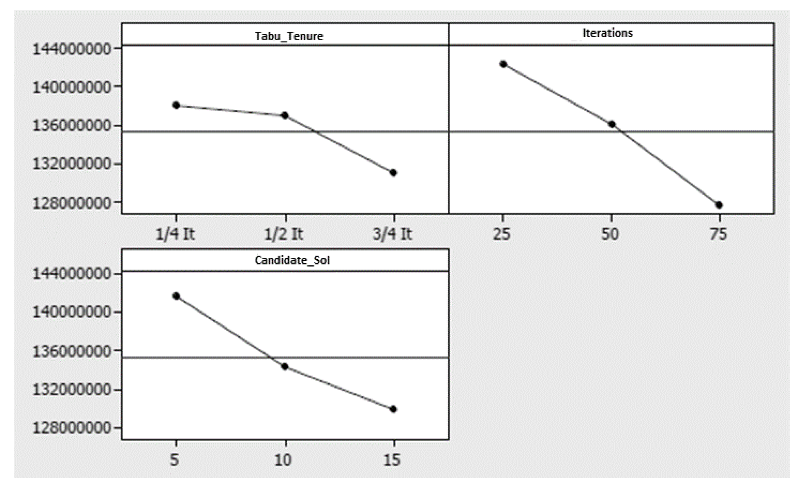
Main effects plots allowed selection of the levels for the experimental factors that minimized the total planning cost. As shown in Figure 3, a larger number of iterations, candidate solutions per iteration, and Tabu tenure, led to better quality results. In this case, experimentation was cost-driven and the high level for each experimental factor was selected for TLBA experiments.

5.2.2. Total Computational Time

According to the ANOVA results, the number of iterations, the number of candidate solutions, and their interaction $Iterations\ast CandidateSol$ had a statistical effect, in terms of computational time. This result is expected, since these two factors determine the necessary number of cycles for obtaining a solution.

As shown in Figure 4, the computational times were directly proportional to the number of iterations and the number of candidate solutions per iteration.

Tabu tenure and its first-level interactions showed a non-significant effect on computational times: The number of iterations that moves stayed in the Tabu list did not affect the average computational time. This result differs from that presented in Section 5.2.1, as Tabu tenure has an important effect on the total planning cost.

5.3. Computational Results

Matlab (R2017a) was the main development environment for the TLBA. Test instances were generated using pseudo-random number generation, according to the parameters in Table 4.

An initial solution was calculated for every generated test instance, using a lot-for-lot method.

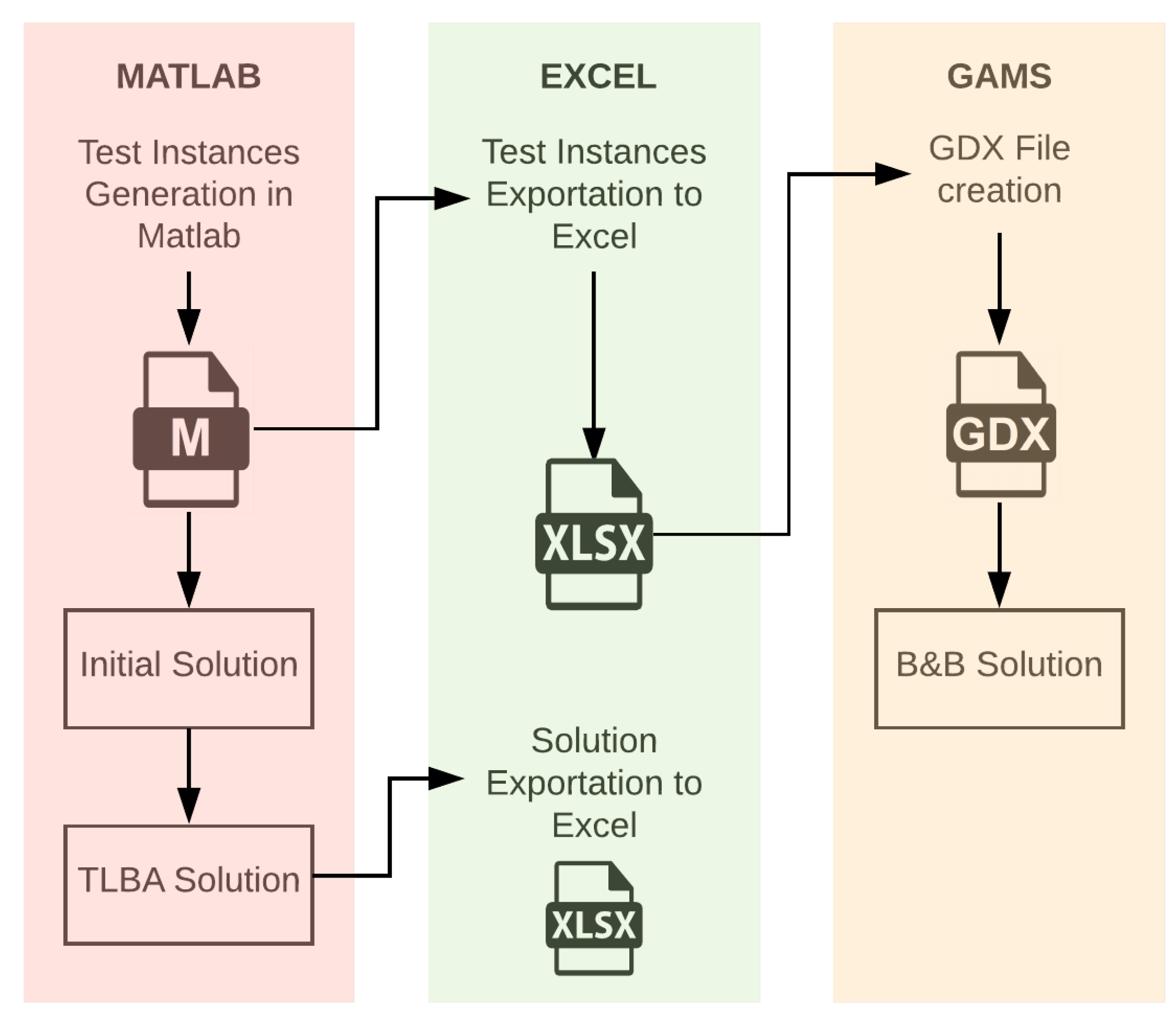
Test instances were exported to spreadsheet files and imported to GAMS using .gdx files. The exact solutions were obtained through a branch-and-bound method using the CPLEX solver in GAMS (version 24.8.2) with default settings. No tolerance settings or time limits were defined.

An overview of the information flow is shown in Figure 5.

The system specifications were as follows:

• RAM: 12 Gb DDR3
• CPU: AMD A6-5200 APU 2.00 GHz
• Operating System: Windows 10 Professional (64 bits)

The results obtained for each of the test instances are shown in

Table 10. Results for total planning cost and total computational times.

Test Instance	B&B GMOP		Initial Solution	TLBA
	Optimal Cost (COP)	Time (secs)	GAP	Min. GAP	Avg. GAP	Min. Comp. Time (secs)	Avg. Comp. Time (secs)
TI1	10,326,117	969.4	14.54	0.2666	0.2952	1424.9	1482.2
TI2	2,683,534	972.5	23.7	0.2757	0.2895	1258.3	1279
TI3	4,890,778	972.8	72.96	0.1659	0.1722	1321.5	1350.2
TI4	106,247,444	994.56	30.23	0.1058	0.1148	7227.1	7260.2
TI5	74,585,367	999.25	10.84	0.1705	0.1773	7741.5	7792.7
TI6	43,278,154	993.24	21.84	0.2871	0.3041	8030.7	8042.5
TI7	1,585,713,234	1001	2.62	0.2186	0.2328	24,959.6	25,002.3
TI8	765,235,068	1020.1	4.66	0.2309	0.3322	27,000.4	27,145.6
TI9	252,626,622	1017.2	16.08	0.1301	0.1486	23,741.6	23,741.6

.

B&B GMOP: Branch-and-Bound solution for the GMOP model.

TLBA: Tabu List-Based Algorithm solution.

Min. Comp. Time: Minimum Computational Time.

Avg. Comp. Time: Average Computational Time.

Gaps were computed using (9), comparing the optimal solutions $C_{Opt}$ with the obtained results in every test instance $C_{Alg}$. Due to the random procedure for moves (see Section 4.4), the average and minimum gaps for TLBA were calculated using five replicas for every test instance.

$$GAP=\frac{C_{Alg}-C_{Opt}}{C_{Opt}}.$$

(9)

6. Discussion

6.1. Solutions Quality

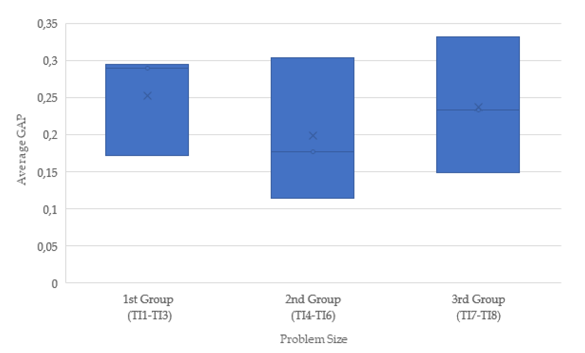
On average, the TLBA was able to obtain solutions with gaps between 11.48% and 33.22% (Table 10). Even when the minimum gaps were obtained in a mid-sized instance (TI4:10.58%) and a large instance (TI9:13.01%), there is no statistical evidence of better performance in a specific problem size.

As shown in Figure 6, the average gaps also showed no significant difference when comparing test instance groups.

Even though the lot-for-lot method allowed for obtaining feasible initial solutions in relatively short times (15–180 s), the gaps for the initial solutions were considerably high. The effect of the initial solution quality on TLBA was not measured, and further experimentation is necessary to improve the algorithm’s efficiency [43,44,45].

Taking into account these results, the exact method remains a convenient option in terms of quality. A cost-benefit analysis may be carried out, due to the sometimes expensive acquisition of solver licenses [10], especially in small and medium enterprises.

6.2. Computational Effort

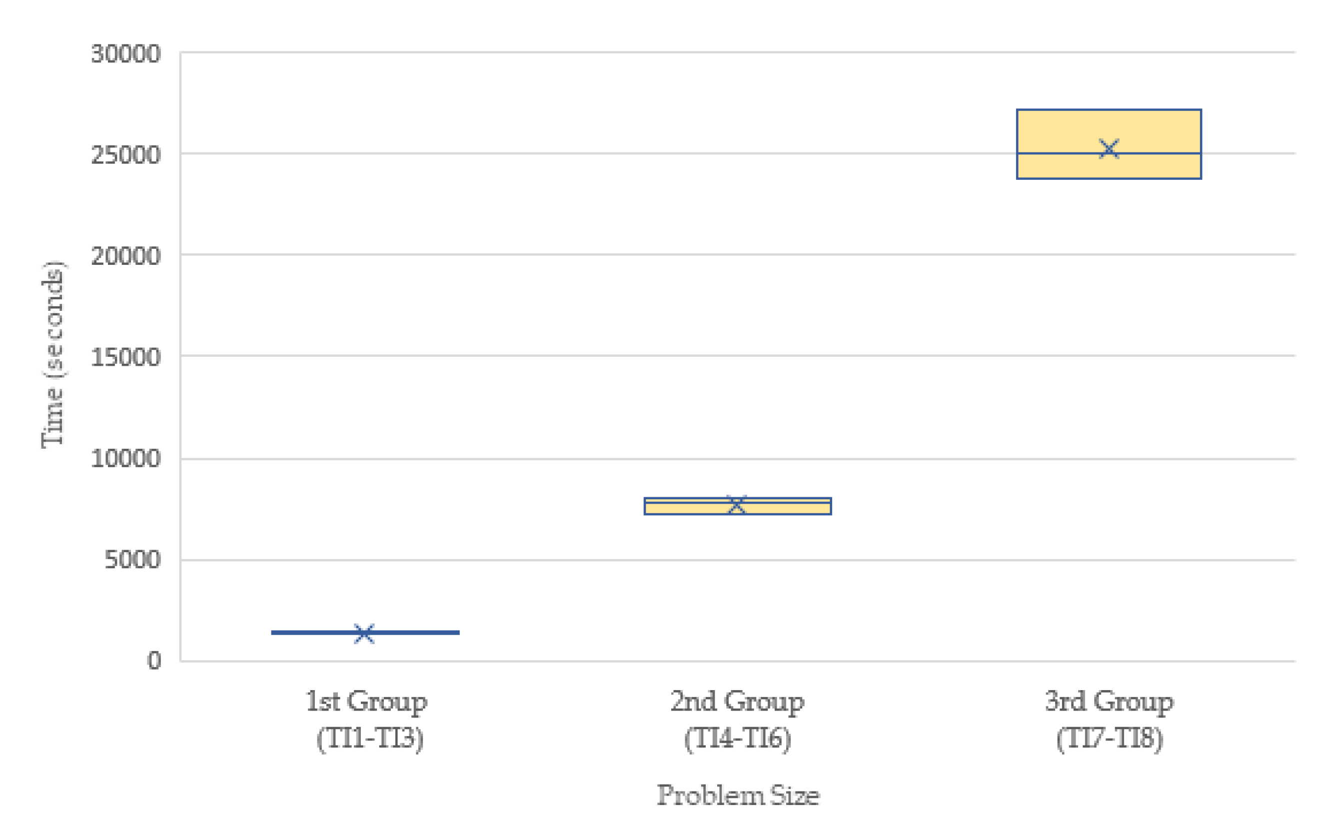
Optimal solutions were obtained in relatively short computational times (970–1020 s), with no statistical difference between problem sizes.

On the other hand, TLBA computational times were higher, with a significant statistical difference among problem sizes, as shown in Figure 7.

As expected, the times were directly proportional to problem size. Only the first instance group showed comparable average computational times with the exact method but, in some cases, the times were up to 52% higher.

Computational times in the medium sized instances were approximately 7 times higher than those obtained with the exact method. In the case of the largest instances, the times increased almost exponentially, with differences near to 2500%.

The solution representation and the evaluation method applied to candidate solutions had a important effect on computational times [46]. The evaluation procedure when obtaining an initial solution was simplified (see Section 4.5), explaining the low computational times in this phase.

In the case of the evaluation procedure for candidate solutions $S_c$ in V, time was basically affected by the number of candidate solutions per iteration $N_s$. It is necessary to analyze the random procedure’s efficiency when obtaining non-forbidden candidate solutions and adding them to V, especially when high values of Tabu tenure are used.

Mutation and combination mechanisms were not considered for generating candidate solutions, this helped to avoid non-feasible candidate solutions related to stroke usage.

The MRP procedure represents the most time-demanding routine. Implementing a more efficient method to obtain SKU inventory levels must be analyzed in further research.

The Tabu list, as a short-term memory mechanism, allowed for improvement in the solution quality. Future work may include the implementation of long-term intensification, diversification, and aspiration mechanisms, in order to improve the algorithm’s performance.

According to the experimental results, Tabu tenure showed no statistical effect on computational times (see Figure 3). This result may imply that, even when the Tabu list optimizes the search, evaluation routines are computationally expensive.

The implementation of TLBA is limited by computational time. However, the use of this kind of procedure would benefit enterprises with low software acquisition budgets (e.g., solver acquisition) having an important efficiency impact on production planning and lot-sizing decisions. This implementation is limited for the understanding and appropriation of the proposed algorithm. Matlab codes, datasets, evaluation procedure, and instance generation algorithms are available in [47] through GitHub.

7. Conclusions

A Tabu list-based algorithm (TLBA) was proposed for the solution of the GMOP model, a capacitated multi-level lot-sizing problem, which considered alternate bills of materials and a controlled co-production environment.

The algorithm obatined solutions with minimum gaps near to 10.5%, in medium-sized instances. The complexity of the data structure, the iterative evaluation procedure for candidate solutions, and the time-consuming calculation for inventory levels were the main three reasons for the large computational times of the TLBA.

Opportunities for future research include the implementation of long-term memory mechanisms for the TS. Additionally, the use of alternative initial solution methods and the improvement of the candidate solution generation procedure may improve the algorithm’s efficiency.

TLBA represents one of the first attempts to find an alternative solution procedure to the established GMOP search algorithms. The use of mathematical approaches (e.g., Lagrangian relaxation and column generation) may result in performance improvements and provide a wide variety of research opportunities.