Evaluation of Deep Learning Neural Networks for Surface Roughness Prediction Using Vibration Signal Analysis

Abstract

The use of surface roughness (Ra) to indicate product quality in the milling process in an intelligent monitoring system applied in-process has been developing. From the considerations of convenient installation and cost-effectiveness, accelerator vibration signals combined with deep learning predictive models for predicting surface roughness is a potential tool. In this paper, three models, namely, Fast Fourier Transform-Deep Neural Networks (FFT-DNN), Fast Fourier Transform Long Short Term Memory Network (FFT-LSTM), and one-dimensional convolutional neural network (1-D CNN), are used to explore the training and prediction performances. Feature extraction plays an important role in the training and predicting results. FFT and the one-dimensional convolution filter, known as 1-D CNN, are employed to extract vibration signals’ raw data. The results show the following: (1) the LSTM model presents the temporal modeling ability to achieve a good performance at higher Ra value and (2) 1-D CNN, which is better at extracting features, exhibits highly accurate prediction performance at lower Ra ranges. Based on the results, vibration signals combined with a deep learning predictive model could be applied to predict the surface roughness in the milling process. Based on this experimental study, the use of prediction of the surface roughness via vibration signals using FFT-LSTM or 1-D CNN is recommended to develop an intelligent system.

1. Introduction

Surface roughness is becoming a significant index to evaluate the quality of products; for example, it is used as an indicator in an in-line monitoring system in the milling process [1]. Surface roughness can also be an indicator to directly monitor the mechanical characteristics of the workpiece, such as fatigue, surface friction, and fracture resistance [2]. The machining parameters affecting the surface roughness are grouped into six major categories: tool properties, work piece properties, machine tool properties, dynamic properties, thermal properties, and cutting properties [3]. Hence, monitoring and predicting the surface roughness in end-milling operations are complex and difficult tasks. Most research studies utilize various intelligent recognition models combined with the inputs of controllable machining parameters, such as feed rate, depth of cut, and spindle speed, to produce a predictive model for the determination of the surface roughness. According to the comprehensive reviews reported in [4,5,6], a classifier/regressive modeling system has been used to classify/predict the surface roughness. However, the remaining five uncontrollable factors of tool properties, work piece properties, machine tool properties, dynamic properties, and thermal properties also affect the surface roughness and thus cannot be neglected during in-process machine milling; this interrelationship makes surface roughness prediction difficult. The above-described predictive models describing the internal representations between the inputs and outputs are formulated using the so-called physics-based or deterministic approach [7,8,9]. T. N. Trung [7] presented the highly nonlinear relationships between processing conditions and the specific cutting energy, arithmetical mean roughness, and means roughness depth. G. Urbikain [8] presented the modelling of surface roughness in inclined milling operations with circle-segment end mills. This study used the most important mechanical and kinematic parameters during cutting. The kinematic parameters include the tool geometry, feed rate, radial immersion, and tool runout. S. Wojciechowski et al. [9] explored the metrological relationships between instant tool displacements and surface roughness during precise ball end milling.

An alternative approach, named the data-driven approach, which involves directly adopting sensor signals’ input data to correlate surface roughness using a statistical and machine learning model, is an approach for predicting the roughness that achieves high accuracy and effectiveness. The crucial factors affecting the performance of the data-driven approach are two-fold: the features extracted for model inputs and the selection of the model used for prediction. Regarding the feature extraction aspects, surface roughness prediction can be achieved directly or indirectly based on various sensor inputs, including images [10,11,12,13], accelerometers [14,15,16,17], and dynamometers [18,19,20,21,22]. S. Ghodrati et al. [11] utilized an image profilometry approach to measure the surface roughness of metallic samples and achieved a highly accurate result. H.H. Shahabi [12] used 2-D images to evaluate the surface profile in the finish machining and successfully forecasted the final surface profile. O. M. Koura [13] applied an image processing technique to measure the surface roughness and explored the effects of the camera resolution and position setting with respect to the measured surfaces. Plaza, E.G. [14] proposed the use of singular spectrum analysis (SSA) to perform surface roughness monitoring based on vibration signals. M. Elangovana et al. [15] proposed the use of multiple regression results to predict the surface roughness and found that the features extracted from the signals were an important index to enhance the reliability of the regression model. Chen, C.C. et al. [16] applied Singular spectrum analysis (SSA) to extract the raw vibration signals and found a correlation between the surface roughnesses in end-milling processing. D. R. Salgado [17] proposed the use of least-squares support vector machines to determine the surface roughness based on cutting vibrations in turning operation. E. D. Kirby et al. [18] used fuzzy-net models for the prediction of the surface roughness, in which the feed rate, spindle speed, and tangential vibration were treated as model inputs. A. K. Ghani et al. [19] investigated the main cutting force and radial cutting force affecting the vibration of the flank wear. M. Thomas et al. [21] investigated the correlation between the cutting force and the surface roughness. K. A. Risbood [22] measured the cutting force and vibrations for predicting the surface roughness in turning operation. In general, dynamometer force sensors are generally large, expensive, and inconvenient to install. Vision image acquisition visualizes the surface roughness and directly predicts it; however, the system is unsuitable in a harsh environment, e.g., fogging via sputtered cooling oil and cooling water. Recently, in the development of an in-process and intelligent surface roughness prediction system, vibration signals of tool condition induced by a workpiece during milling operation are being used for surface roughness prediction. The interaction of all the machine parameters acting on the workpiece allow acquiring the vibration signal information generated from a machine tool body embedded with an accelerometer. The complex internal relations between surface roughness and machining parameters can be determined in the formulation of the surface roughness correlated with vibration signals using high performance prediction models. Based on observation, vibration signals are highly correlated with surface roughness in nature. Several researchers have used different vibration signals to predict the surface roughness [23,24,25]. H. H. Luke et al. [24] constructed a multiple regression model to predict the in-process surface roughness of the workpiece in the turning operation based on vibration amplitudes, feed rate, depth of cut, and spindle speed; the result of the predicted accuracy was as high as 90%. O. B. Abouelatta [25] proposed mathematical models for predicting surface roughness based on machine tool vibrations and cutting parameters and used the models to observe the correlation between cutting vibrations and surface roughness. The above-described studies revealed that the prediction of surface roughness can be achieved by using vibration signals. The developed intelligent monitoring surface roughness system based on vibration signals could not only directly acquire the in-process surface roughness, but also ensure both the quality and quantity of the machined product. Thus, the aim of this research study is to verify the efficacy of a surface roughness prediction system based on the use of vibration signals.

Recently, artificial intelligence (AI) techniques have been applied in vibration analysis. The AI technique is able to learn significant features from original historical data and can make a decision based on on-line data. Vibration analysis based on the AI technique usually involves four steps: data acquisition, feature extraction, model training, and model testing. The methods most commonly used for feature extraction methods are time-domain, frequency domain, and time-frequency domain methods. The extracted features are fed into the classifier, such as a support vector machine (SVM) [26,27,28] or a neural network (NN) [29,30]. N. N. Bhat [26] proposed the use of the SVM technique for classifying tool wear states of surface images. J. Sun et al. [27] used the SVM approach to identify tool flank wear. S. Cho [28] proposed the use of the SVM algorithm to identify tool breakage abnormalities. H. Q. Wang [29] proposed a sequential diagnosis approach using the partially-linearized neural network to identify the fault rolling element bearing. S. G. Barad et al. [30] proposed a neural network technique to monitor the health of a power turbine. Surjya K. Pal [31] used a back propagation neural network model to predict the surface roughness in turning. D. R. Salgado [17] employed the least-squares SVM method along with the cutting conditions (feed rate, cutting speed, depth of cut) and the vibration signal feature to estimate an in-process surface roughness in turning processes. Considering the sensitivity of vibration signals to the background noise, signal analysis using the convection signal condition method is ineffective. Moreover, different features of vibration signals are extracted manually, resulting in the problem of low generality. An effective feature extractor is required to automatically extract useful signal features. In addition, the conventional predictive models belong to shallow layer structures, making it difficult to learn the complex nonlinear relationships involved in vibration signal prediction problems. Researchers have investigated the use of a convoluted features extractor and deep architecture to make significant progress in various application fields. The multi hidden network architecture proposed by the pioneer Hinton [32] possesses the following outstanding advantages. Deep layers in the convolution operator could extract important features from raw data and preserve the characteristics of parallel computing and self-learning features in shallow networks that could explore more natural feature information from complex data. Explosive applications are expanded in the signal analysis and machine fault detection problems. H. Pan et al. [33] used one-dimensional convolutional neural network (1-D CNN) and long short term memory (LSTM) for vibration signal analysis to perform bearing fault diagnosis. K. Li et al. [34] used a 1-D CNN model with raw data to perform real-time motor fault detection. Z. Rio et al. [35] designed a deep LSTM model to predict the actual tool wear based on raw sensory data. Although deep learning techniques have been widely applied in the machinery industry, little effort has been applied to predicting the surface roughness of a monitoring system during the milling process using deep learning architecture. The two types of deep learning models—convolutional neural network (CNN) [34,36] and LSTM [33]—have had their outstanding performances tested and verified in detection and classification for fault diagnosis of rotating machines. In this paper, we study these three predictive models to predict the surface roughness based on the vibration signals in the milling process.

For a machine monitoring system used in the milling process, measuring vibration signals based on sensory data is a characteristic task. A conventional model prediction method, such as neural network and SVM, cannot express the sequential features extracted from serious vibration signals. LSTM can deal with the different lengths of data in sequential time and extract long-term series features for postprocessing. The deep training structure is capable of recognizing unseen data and thus can be used to generalize the predictive model. Although LSTM considers sequential data characteristics, some shortcomings of the model may not allow it to achieve robust prediction based on raw sensory data. As suggested by Rui. Zhao et al. [37], the raw data converted from time-domain signals to frequency domain spectrum features are fed into the LSTM to achieve high performance in prediction. In addition, a report in the literature [38] showed that CNNs, LSTMs, and Deep Neural Networks (DNNs) have respective prediction capabilities: CNNs are capable of filtering signal noise by convolutional filters and pooling operations, LSTMs can deal with temporal modeling, and DNNs are appropriate for mapping features in multidimensional space. The objective of this research is to study the Fast Fourier Transform (FFT) extractor and the one-dimensional convolutional extractor combined with three predictive models, namely, FFT-DNN, FFT-LSTM, and 1-D CNN, to predict the surface roughness via vibration signal information. This paper is organized as follows: Section 2 presents details on the research methodology and describes the structure of each of the models. Section 3 describes the experimental setup. Section 4 presents the experimental results. Section 5 summarizes this article.

2. Research Methodology

The core objective of this research is to predict the surface roughness via vibration signals. Thus, the historical data of vibration signals are used as the input data, and the output data is defined as the surface roughness of the workpiece. The prediction model is designed to identify the relationship between the vibration signals and the surface roughness value. The model can further infer the surface roughness based on the in-process vibration signals. The key factors that affect the performance of AI techniques are the features used and the designed models. The conventional features extracted from time-domain raw data are the following nine features: mean, root mean square, variance, peak value, peak to peak value, kurtosis, skewness, crest factor, and impulse factor [33]. In our previous studies, poor results were obtained for the above nine features extracted from the raw vibration signal data using the trained DNN and LSTM models. Thus, advanced alternative features are used in the DNN, LSTM, and CNN models. The methodology used in this article involves two primary sections, one is the feature extractor method, and the other is the use of a popular regression model. Figure 1 shows the framework of this research study. The sensory data of signal vibration are extracted as the model inputs, and three models are adopted to predict the surface roughness. First, the FFT is used as the feature extractor, and then these features are fed into the deep neural network predictive model. Second, the FFT is combined with LSTM to extract the features, and then the fully connected networks (FCN) approach is used to perform the regression task from vibration signals. Third, the 1-D CNN model based on time vibration signals is adopted for prediction. The details of these approaches are presented below.

2.1. FFT-LSTM-FCN

The studied model presented here is an LSTM model that belongs to a regression problem of sequential property and is adapted in our research study to achieve superior results. LSTM has the potential to recall the previous time series data and has the advantage of being able to determine whether the features are important. Several reports in the literature indicated that the LSTM model cannot deal with raw data; as a result, the FFT is combined with the LSTM model to extract the represented features in the present investigation. The framework of the LSTM model is shown in Figure 2. There are three main gates to control the cell state. The input gate controlling the new information can be stored in the cell; this process can be expressed by Equations (1) and (2). The forget gate controlling the previous information can be discarded from the cell; this process can be expressed by Equation (3). The output gate determines the information extracted from the cell; this process can be expressed by Equations (4)–(6). The LSTM model, combined with a fully connected network, makes a decision. The equations of the LSTM model used in present paper are as follows:

$$i_t=\sigma (W_i[h_{t-1},x_t]+b_i)$$

(1)

$${\stackrel{\sim }{C}}_t=\tanh (W_C[h_{t-1},x_t]+b_C)$$

(2)

$$f_t=\sigma (W_f[h_{t-1},x_t]+b_f)$$

(3)

$$C_t=f_t{C}_{t-1}+i_t{\stackrel{\sim }{C}}_t$$

(4)

$$o_t=\sigma (W_o[h_{t-1},x_t]+b_o)$$

(5)

$$h_t=o_t\tanh (C_t)$$

(6)

where $i_t$ is the input gate, $\mathsf{\sigma }$ is a sigmoid function, $W$ is the weighting factor, $h_{t-1}$ is the cell output, $b$ is the bias, $f_t$ is the forget gate, and $O_t$ is the output gate.

2.2. 1-D CNN

Fourier transform has been the most popular feature extraction method used in analyzing signals. The one-dimensional convolution function in 1-D CNN can be similarly treated as the wavelet transform; thus, the convolutional neural network model achieves efficient performance in extracting the raw signal waveforms [39]. The greatest advantage of this method is that it does not require any feature extractors of transformation. This method can directly process the raw data. To extract the features automatically from the raw vibration signals, this study utilizes the 1-D CNN structure to extract the features. Figure 3 illustrates the 1-D CNN model.

1-D CNN is composed of the following: input layer, convolutional layer, pooling layer, FCN layer, and output layer. The convolutional layer is the first layer that is used to extract features from the raw data, which could be reduced to sparse feature maps via convolutional kernels. The processing of the vibration signals is a sequential data analysis problem, for which one-dimensional kernels are adapted in this research. This model performs the one-dimensional filter operation by sliding over the sequence data to obtain the corresponding feature maps. Next, the max pooling operation is used to determine the maximum value of the feature maps. The output of the convolutional layer and the max pooling operation can be expressed as follows:

$$Y_{m,k}=f\left({\displaystyle \sum _{i=1}^n{x}_i\ast }{w}_m+b\right)$$

(7)

$${\mathrm{Z}}_{m,L}=\max (Y_{m,k})$$

(8)

where, $Y_{m,k}$ is the output of the convolutional layer, $X_i$ is the sample number, $W_m$ is the convolutional kernels size, $b$ is the bias, and $f$ is the activation function. This experiment uses the max pooling operation as the pooling layer; thus, $Z_{m,L}$ is the output of the pooling layer.

3. Experiments

In this section, the performance of the proposed method is evaluated. First, each dataset is described. Next, the details of the experimental setup are given. Finally, the results of each method are discussed and analyzed.

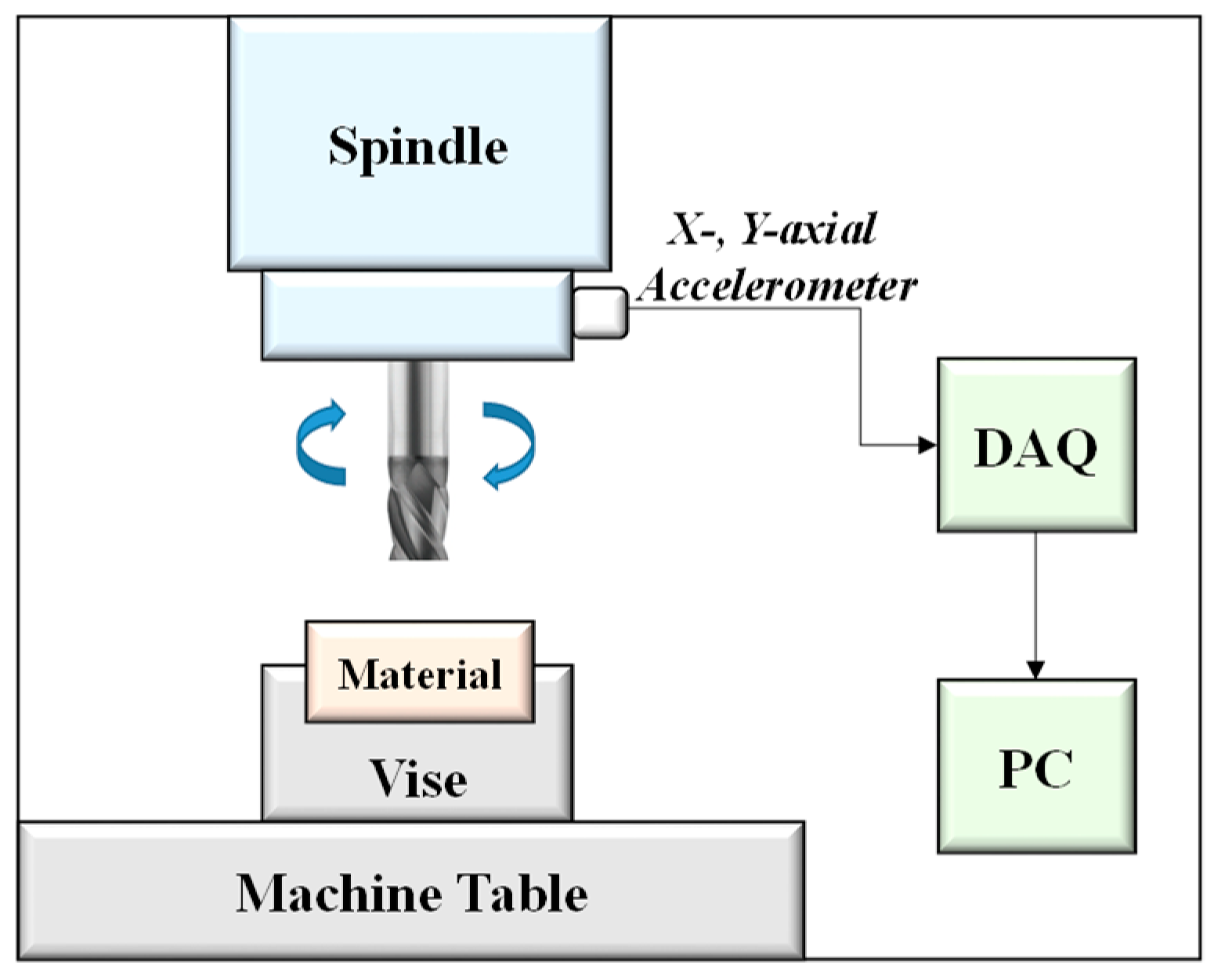
3.1. Dataset Descriptions

This study evaluates the performance of three predictive models with vibration signals generated during milling operation of a CNC machine. The flowchart of the experimental platform is shown in Figure 4. First, vibration signal data are acquired from an acceleration sensor when the cutter starts to mill the workpiece. Subsequently, three predictive models are trained using the input of vibration signal data. The evaluation of the training and prediction results will be used to compare the models. Figure 5 shows the experimental setup; sensory data are obtained from the X and Y directions of the accelerometer (50 g) attached in a spindle tool as the vibration signals for analysis. For simplifying the analysis of the correlation between the vibration signals and the surface roughness in the intelligent predicted model considered here, the machine parameters are set at the special milling conditions as follows:

(a)

The material of the workpiece is Medium-Carbon Steel S45C, and the material of bull end billing tool is AlTiN Coated Carbide with axial depth of cut (ap) of 2 mm and radial depth of cut (ae) of 10 mm;

(b)

The final finish milling depth of 10 µm in this process was used to obtain the vibration signals in the experiment;

(c)

The center spindle speed is set at 7000 rpm;

(d)

10 KS/s is chosen as a sampling rate, such that the raw vibration data sampling rate is 10 k in one second;

(e)

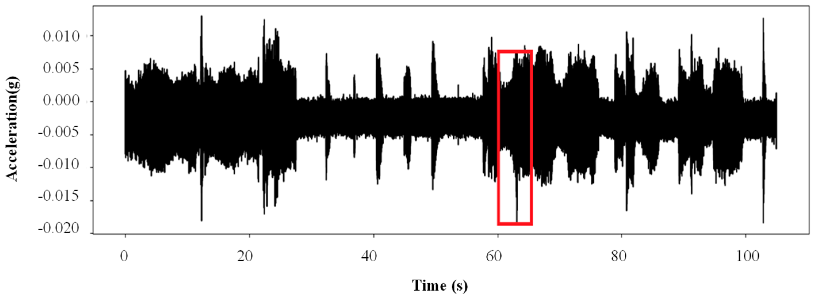
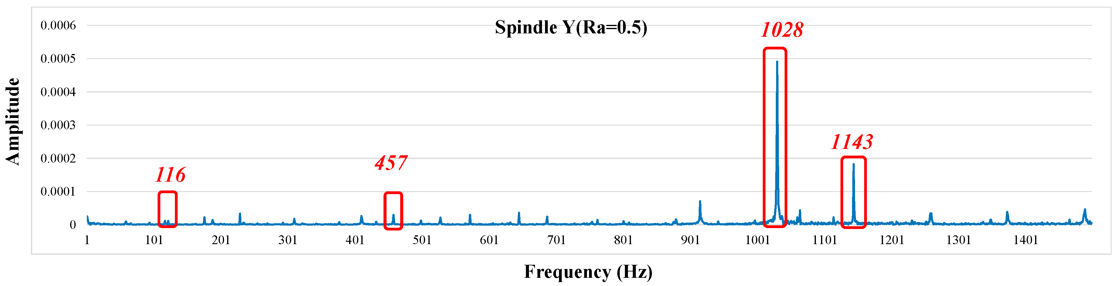
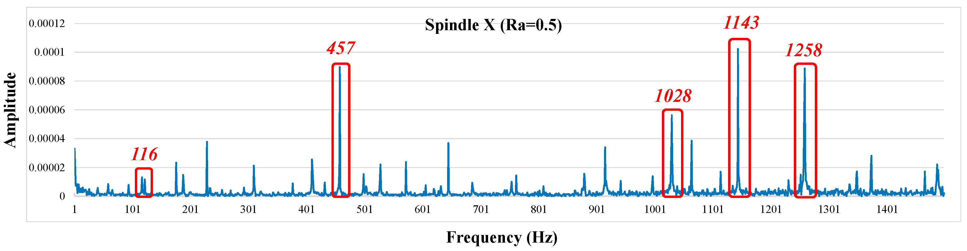
The selected five seconds of sample data are taken between 63 s and 68 s, corresponding to the end of the milling process. The vibration signals sampled with the 5-s time interval are highlighted by the red box in Figure 6. Two-axis accelerometers are used in this experiment; thus, x- and y-axial vibrations are produced during milling operation. The x- and y-axial vibrations are converted to Fourier spectra, as shown in Figure 7 and Figure 8. The vibration signal features in the spectrum signals of the x and y accelerations are partially consistent in processing time. However, the spectral features from the x-axis have rich feature information that is more sensitive in the milling processing. For simplicity, in this study, only vibration signals in x-axial direction are used as model inputs to predict the surface roughness.

(f)

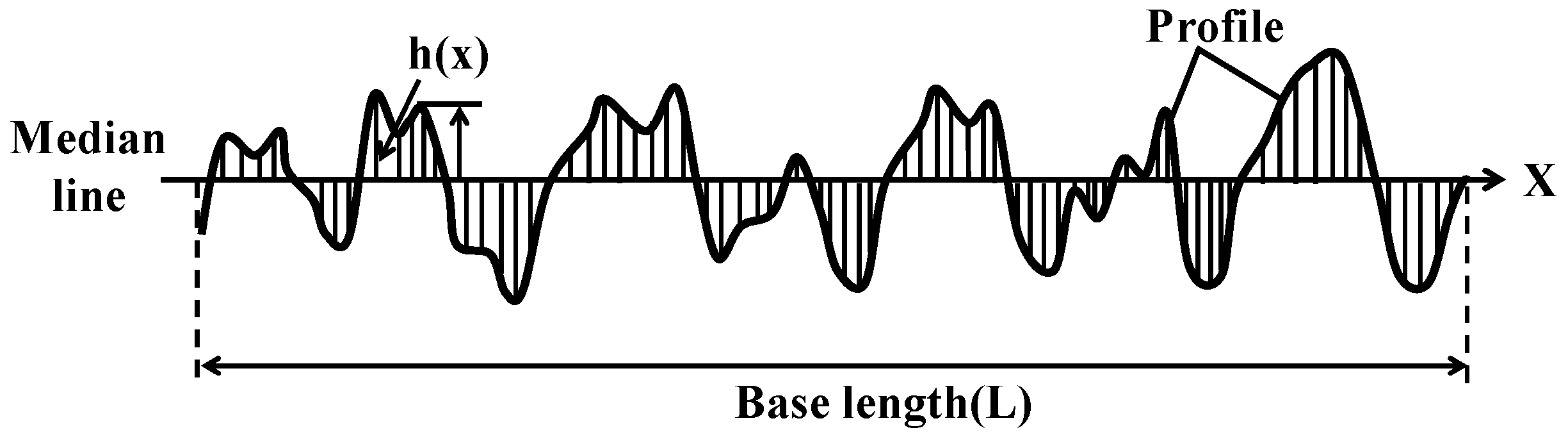
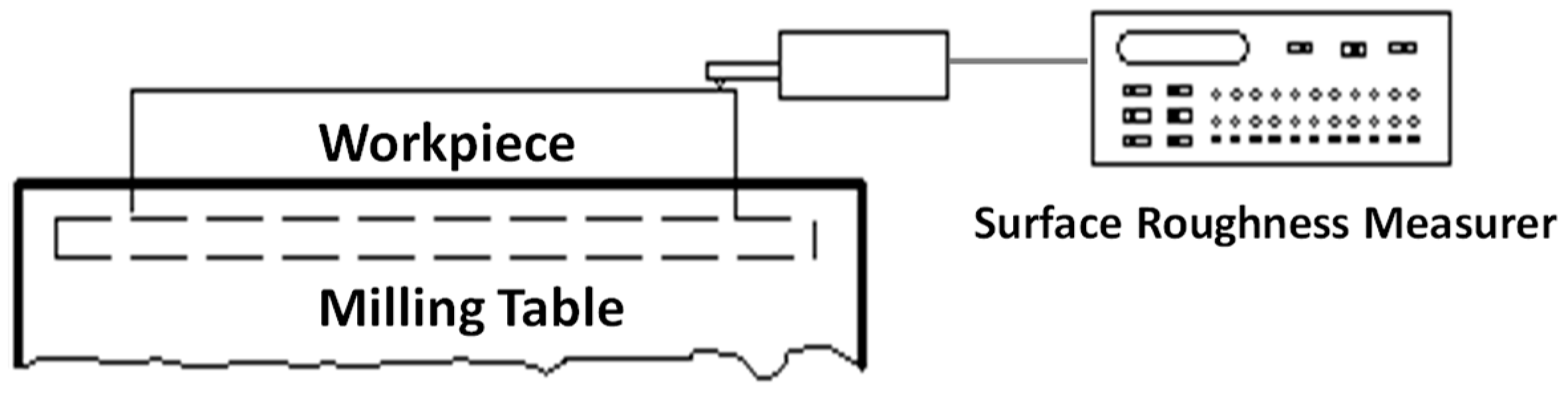
The surface roughness (Ra) in the milling processing was measured offline by a 2-D surface roughness measurer (SV-3200 Series). Ra value is defined as Equation (9), where $h\left(x\right)$ is the surface waviness profile and $L$ is the measured length. Figure 9 presents the plots and definitions of the surface roughness profile. Figure 10 shows the measurement system of surface roughness.

$$Ra=\frac{1}{L}{{\displaystyle \int }}_0^L\left|h\left(x\right)\right|dx$$

(9)

3.2. Dataset Preparation

Extracting represented features for the input layer is a crucial step to achieve good prediction. Data extraction is separated into two parts in this study. The FFT transform method is used for extracting the raw data, and the other approach of 1-D CNN automatically extracts the raw vibration signals as the input data. The raw data before being fed into FFT extractor is 10k samples per second, corresponding to a total of 50k samples for a sampling time of 5 s. After FFT operation, the spectral data is reduced to 5000 Hz as the feature data of the input layer. The spindle speeds of 116.6 Hz (7000 rpm) captured by the accelerometer, as shown in Figure 7 and Figure 8, appear to be very small compared with others, indicating that the spindle rotatory machine has balanced performance. The spectrum was extended to approximately 1500 Hz based on a factor of 10 used to account for the vibration spectrum of the machine milling process. The machine tool with four flutes used in the milling process strikes the workpiece approximately 465 times per second (116.6 Hz × 4), resulting in the higher spectral amplitude depicted in Figure 7 and Figure 8. Other features in the spectral distributions are considered as important signal features for training the studied models. In addition, 1D CNN is employed to automatically extract the raw vibration signal data; thus, the total number of samples of data for analysis is 10,000.

In this experiment, the 50 workpiece datasets arranged at special milling process conditions are used to obtain 50 sets of vibration signal data for evaluation of the surface roughness prediction using deep learning neural networks.

3.3. Model Setup

To investigate the performance of the surface roughness predictive model, three different models are considered in the present research study: (1) combine the FFT extractor with the DNN model; (2) combine FFT and the LSTM model; and (3) utilize the one-dimensional CNN model. The designed parameters of each of the models are presented below.

Because DNN and LSTM could not deal with raw data, the FFT feature extractor is used at the beginning. After the FFT feature extractor is used, the represented vibration spectrum has 1500 spectrum feature inputs. The 50 datasets are further used for training and testing to implement the relevant regression predictive model, i.e., DNN of LSTM. For the DNN model, the study involves four fully connected layers with layer sizes of [12288, 6144, 6144, 1], and the activation function of each layer is set as ReLU. For the LSTM model, the deep layers of LSTM are conducted with 2048 cells in sequence, and the learning rate is set as 0.0035. For the 1-D CNN model, this model is composed of the following: one convolutional layer, a max pooling layer, and fully connected neural networks. The hyper parameters of the 1-D CNN of kernel size, kernel numbers, strides, learning rate, and padding are set as 500, 16, 300, 0.0035, and 250, respectively.

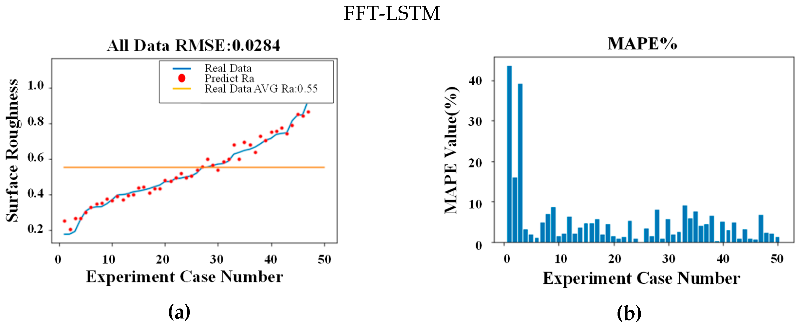
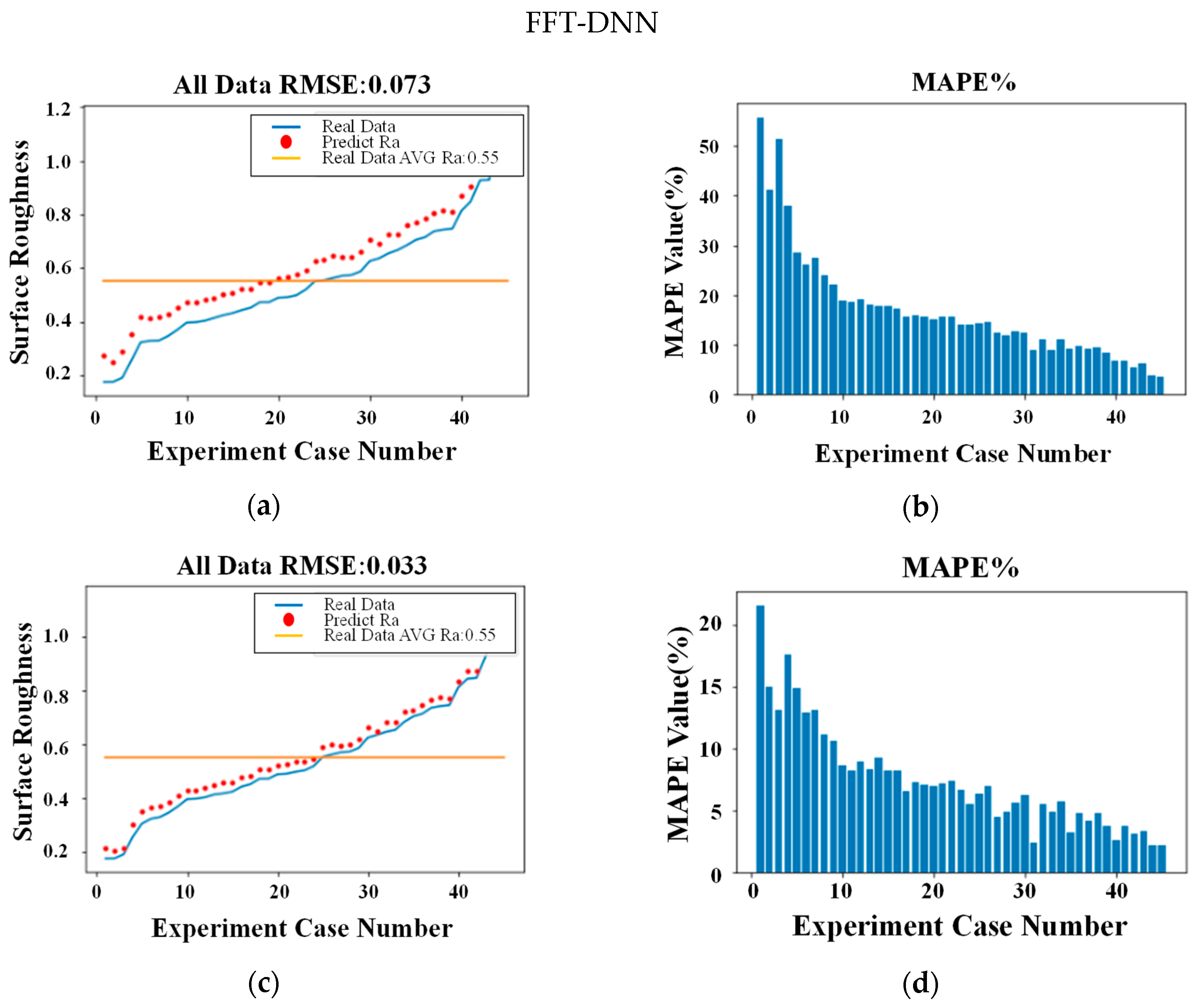
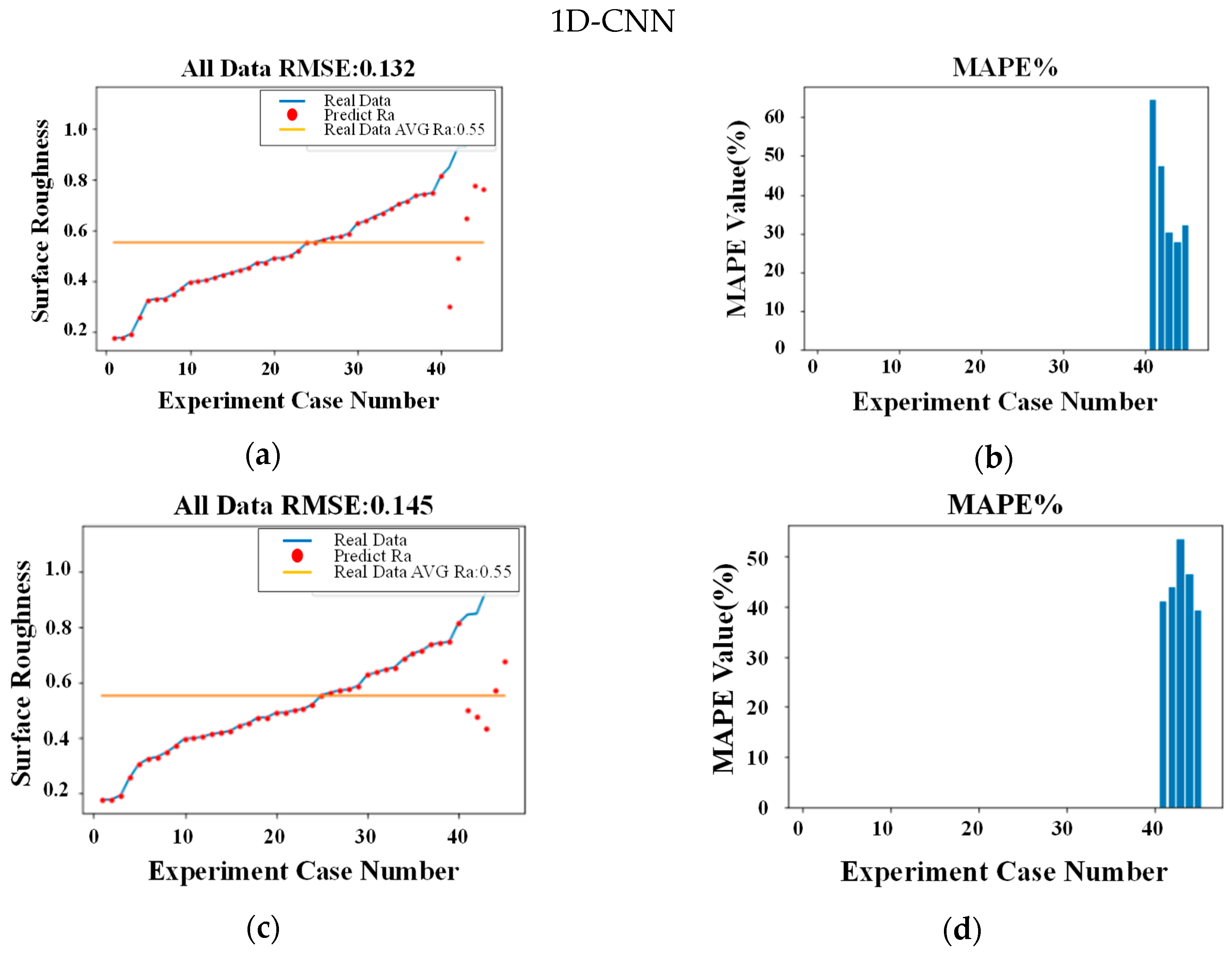
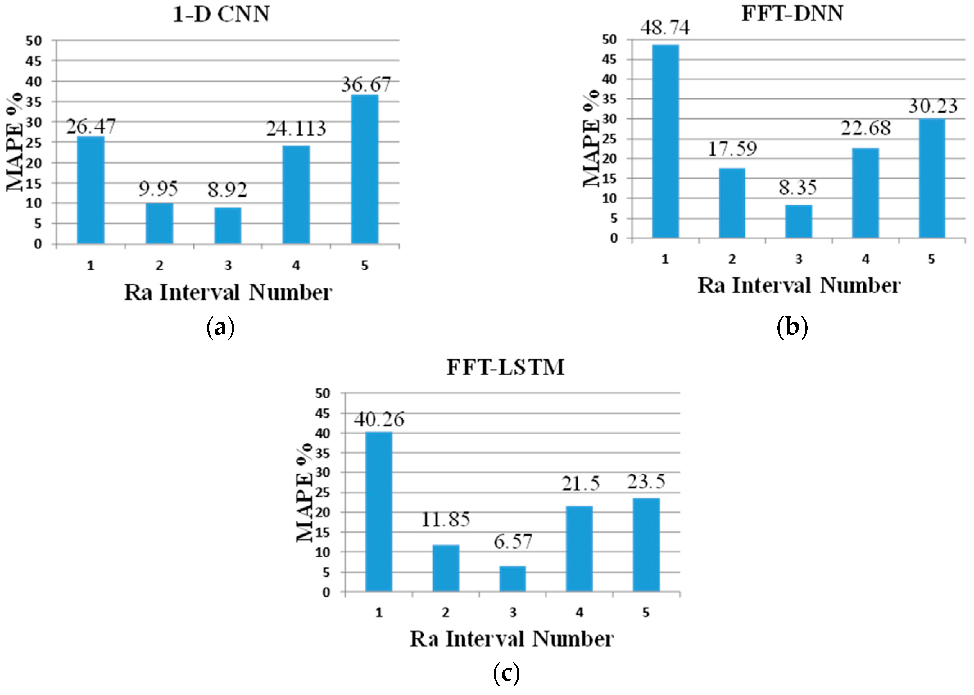
4. Experimental Results on Surface Roughness Prediction

Evaluations of the performance on surface roughness using deep learning networks are two-fold. Considering the insufficient datasets obtained here, the datasets for evaluating the present predictive model are arranged into two strategies. The first step in the experiment takes all sample datasets to be trained and evaluates the training performance of the loss function and regressive deviation indicated by root-mean-square error (RMSE) and mean absolute percentage error (MAPE). The cross-validation method is typically used for visualizing the training score in training process under insufficient dataset conditions. Similarly, this study involved the use of cross-validation to predict the accuracy after finishing the training. Hence, the second step divides all sample datasets into 45 datasets for training and 5 unseen datasets for testing the prediction accuracy.

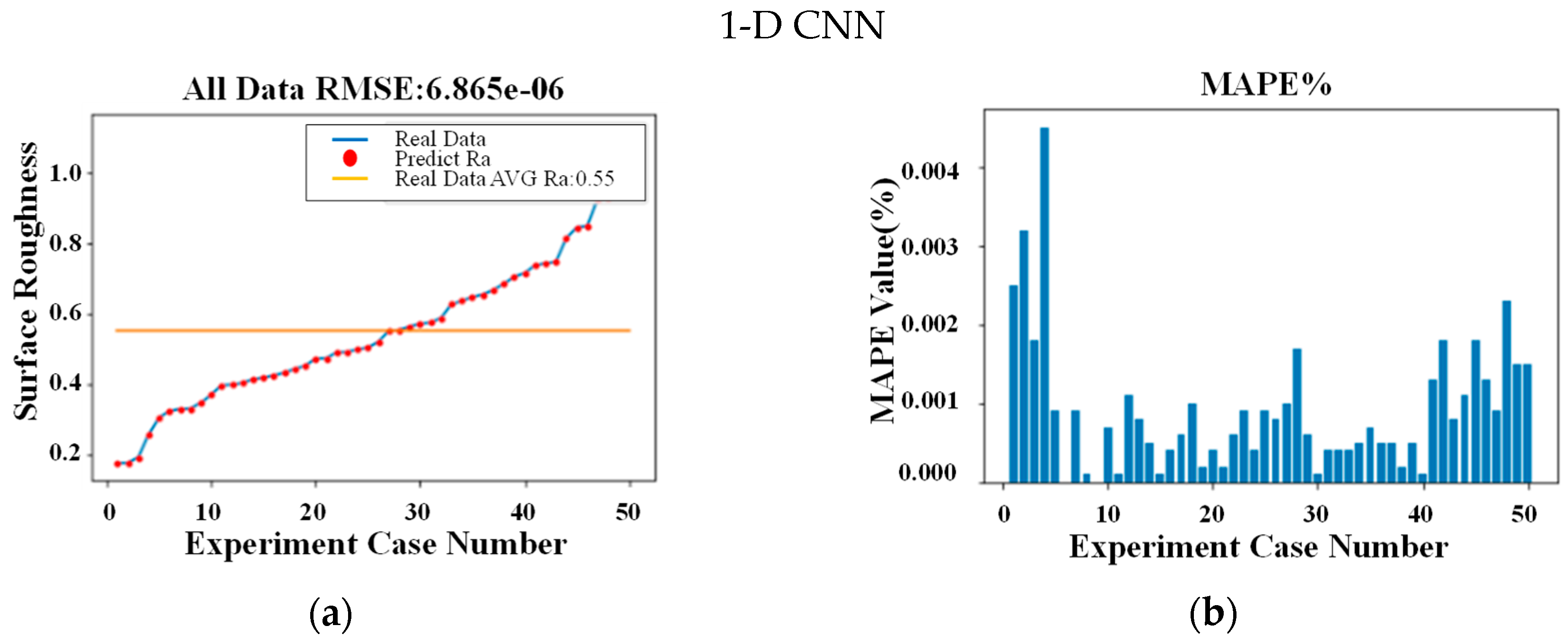
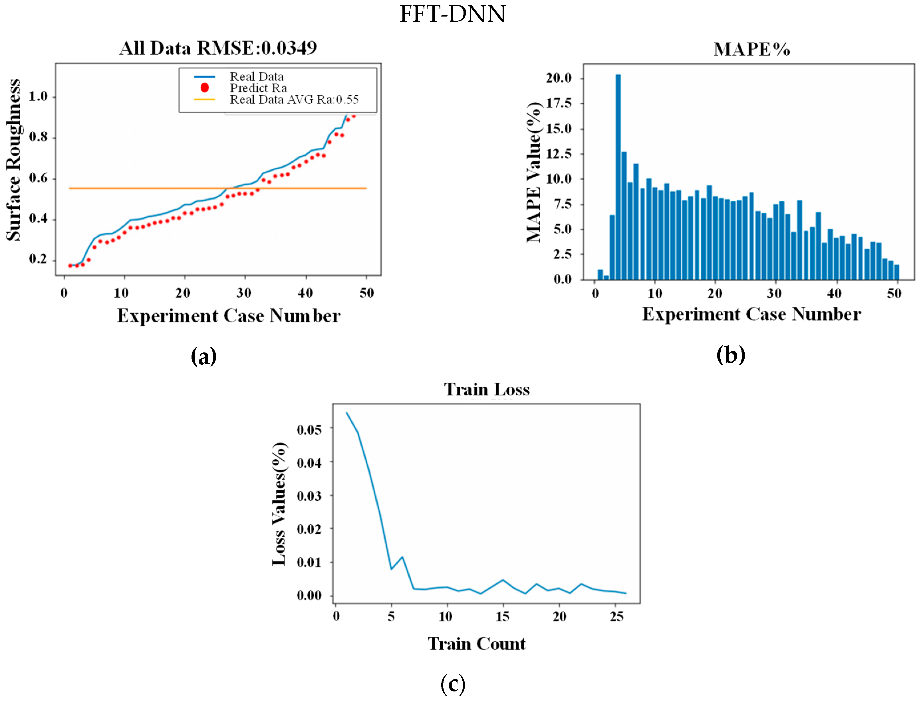
Performance of the Three Applied Models

To demonstrate the learning effectiveness of the three predictive models in the training process, all datasets gathered under the circumstances of limited resources are employed to perform the analysis. The loss function distributions exhibit convergent efficiency and accuracy in the optimum learning process. The loss function results of 1-D CNN, as shown in Figure 11c, demonstrate a stable convergence process and attain a considerably small convergence value. The other two models, FFT-DNN in Figure 12c and FFT-LSTM in Figure 13c, exhibit small fluctuating distributions in the convergence process; however, they still achieve an accepted convergence value. Comparison of the convergence performance of the three models indicates that the 1-D CNN model is the best because of its improved feature extraction capability compared to the FFT-DNN and FFT-LSTM models using the FFT feature extractor. Further, all three of the models can obtain rather low convergent values in the learning process. In the comparison of the regression predictive accuracy in the learning results, the RMSE and MAPE utilized to assess the surface roughness prediction value are defined in Equations (10) and (11). The results of each of the models are shown in

Table 1. The RMSE and MAPE of training results.

Present Model	RMSE	Average MAPE(%)
FFT-DNN	0.0349	6.827
FFT-LSTM	0.0284	5.224
1-D CNN	0.000006	0.0009

, the individual self-regression-predicted Ra is plotted (red) in Figure 11a to Figure 13a, and the regression-predicted Ra error is depicted in Figure 11b to Figure 13b. 1-D CNN achieves the best performance of the learning results, with the learning datasets almost completely fitting the predicted data. From the self-prediction result using the learning regression model, the three models exhibit high learning capability, with 1-D CNN found to achieve superior feature extraction in the present study.

$$\mathrm{MAPE}=\frac{1}{n}{{\displaystyle \sum }}_{i=1}^n\left|\frac{y_i-x_i}{y_i}\right|\ast 100\%,$$

(10)

$$\mathrm{RMSE}=\sqrt{\frac{{{\displaystyle \sum }}_{i=1}^n{\left(y_i-x_i\right)}^2}{n}},$$

(11)

where $n$ is the experiment case number, $y_i$ is the real Ra value, and $x_i$ is the predicted Ra value.

To validate the ability of the predictive models, training models must be tested to verify the generalization in actual prediction. In the limited data conditions, a total of 50 vibration signal datasets are separated into 45 datasets for training and 5 datasets for testing. First, datasets are sorted by Ra value from small to large and annotated from No. 1 to No. 50. As arranged in

Table 2. Surface roughness (Ra) datasets.

(Interval Number) (Annotated Number)		$\mathbf{Ra}\left(\mathit{\mu }\mathit{m}\right)$
(1) (1~10)	Lower Ra	0.177	0.177	0.192	0.257	0.306	0.324	0.329	0.331	0.347	0.370
(2) (11~20)	Medium Ra	0.397	0.399	0.404	0.414	0.418	0.425	0.432	0.443	0.453	0.473
(3) (21~30)		0.473	0.490	0.492	0.499	0.504	0.520	0.551	0.554	0.563	0.571
(4) (31~40)		0.574	0.588	0.626	0.636	0.647	0.654	0.667	0.684	0.705	0.714
(5) (41~50)	Higher Ra	0.737	0.743	0.747	0.814	0.845	0.848	0.926	0.928	1.073	1.118

, the Ra samples are divided into five intervals, with each interval containing 10 datasets. The lower/higher Ra range are in interval No. 1/No. 5, and the medium Ra range are in interval No. 2 to No. 4. In general, the Ra value is separated into three levels, with the lower/higher range having less/greater than 0.4/0.7 Ra value, and 0.4 to 0.7 Ra value belongs to medium level. Defining the lower, medium, and higher ranges of surface roughness is helpful for the following quantification analysis. The five testing datasets are regularly chosen in each of the intervals, and the remaining 45 datasets are used for training. For example, datasets numbered (4, 14, 24, 34, 44) and (6, 16, 26, 36, 46) are selected as the testing datasets. The training results corresponding to FFT-DNN, FFT-LSTM, and 1-D CNN using the remaining datasets are displayed in Figure 14, Figure 15 and Figure 16, respectively. All three models converge to a low loss function in the training process. However, the self-prediction of the 1-D CNN model is not found over the range of Ra values available here. Figure 14a,c correspond to datasets of numbers (4, 14, 24, 34, 44) and (6, 16, 26, 36, 46), respectively.

Error analysis in training and prediction are used to explore the performance of each model in the present study. The self-predictive model after training performs effectively at lower and approximately mean Ra value, but suffers from poor learning prediction problems for higher Ra values. In practice, higher Ra values correspond to violent vibration signals. The 1-D CNN model, which essentially extracts abundant feature data with sufficient datasets, served as a superior predictive model. In the case of the lack of datasets in this study, under-fitting results appear at higher Ra values in the training process. FFT-LSTM and FFT-DNN could be well-trained over a range of Ra values using a weak feature extractor for few datasets. To compare FFT-LSTM and FFT-DNN with the same FFT extractor, the training results are displayed in Figure 14a,b for the FFT-DNN, and Figure 15a,b for the FFT-LSTM, respectively; FFT-LSTM, with the same training datasets, shows that FFT-DNN presents higher deviations over all training datasets. FFT-LSTM outperforms the training effectiveness of the 1-D CNN model in the training process.

Finally, cross-validation for testing is performed to evaluate the predictive performance of the surface roughness via vibration signal datasets after training datasets. Using the afore-described methods for choosing the test dataset numbers, dataset numbers (3, 13, 23, 33, 43), (4, 14, 24, 34, 44), (5, 15, 25, 35, 45), (6, 16, 26, 36, 46), and (7, 17, 27, 37, 47) are chosen for testing the datasets to account for cross-validation in the testing process. The mean error results of the dataset cross-validation is provided to evaluate the predictive accuracy of the trained model. The criteria of prediction performance presented in [40] declare that MAPE ranges from less 10%, 10%–20%, 20%–50%, and greater 50% response correspond to highly accurate, accurate, reasonable, and not accurate predictions, respectively. An overview of the results of the three predictive models is shown in Figure 17a to Figure 17c. FFT-LSTM achieves the best predictive performance over Ra values in the studied Ra range. Moreover, the three models have poor predictive capability for lower Ra range and higher Ra range. Overall, the FFT-DNN with 48.75% MAPE at lower Ra range falls into the not accurate predictive level. Excluding the lower and higher Ra ranges, the three models are at the accurate predictive level. Moreover, the predictive performance of 1-D CNN obtained a highly accurate level in the medium Ra range, 9.95%, and 8.92% MAPE, as shown in Figure 17a. The higher Ra range prediction of FFT-LSTM exhibits preferred results in comparison with the three models. These findings reveal that FFT-LSTM takes advantage of temporal modeling to present forecasting in the high Ra range. At lower Ra ranges, 1-D CNN achieves the best predictive ability because this model can extract insensitive feature information; this ability is helpful for prediction in high-precision milling processes.

5. Conclusions

This paper presented an evaluation of the deep learning approach to determine surface roughness using vibration signal data. The three predictive models of 1-D CNN, FFT-DNN, and FFT-LSTM were evaluated in terms of their training and prediction performances. The results are summarized as follows. All three models have good training performance in sufficient data conditions, with 1-D CNN exhibiting superior training performance. After training the models, the predictive performance of all the three models achieve satisfactory accuracy with less than 20% MAPE at medium Ra ranges between 0.4 to 0.7. Comparing the three predictive models, FFT-DNN has the worst prediction at the lowest Ra range with 48.75% MAPE and 1-D CNN is the worst at the highest Ra range with 36.67% MAPE. 1-D CNN can extract elaborate features to present better prediction ability and achieves a highly accurate level of prediction at lower Ra values with 26.47% MAPE. FFT-LSTM utilizes temporal modeling forecasting to perform well at higher Ra ranges with 23.5% MAPE. Furthermore, the experiments also revealed that 1-D CNN can extract the features automatically and extract more information compared to the FFT extractor. Based on these results, vibration signal data combined with the 1-D CNN and FFT-LSTM models are recommended for prediction of surface roughness during milling processes.

References

1. Huang, B.P.; Chen, J.C.; Li, Y. Artificial-neural-networks based surface roughness Pokayoke system for end-milling operations. Neurocomputing 2008, 71, 544–549. [Google Scholar] [CrossRef]
2. Akhiani, H.; Szpunar, J.A. Effect of surface roughness on the texture and oxidation behavior of Zircaloy-4 cladding tube. Appl. Surf. Sci. 2013, 285, 832–839. [Google Scholar] [CrossRef]
3. Khorasani, A.M.; Yazdi, M.R.S.; Safizadeh, M.S. Analysis of machining parameters effects on surface roughness: A review. Int. J. Comput. Mater. Sci. Surf. Eng. 2012, 5, 68–84. [Google Scholar] [CrossRef]
4. Black, J.T.; Kohser, R.A. DeGarmo’s Materials and Processes in Manufacturing, 11th ed.; Prentice Hall: Upper Saddle River, NJ, USA, 2011. [Google Scholar]
5. Upadhyay, V.; Jain, P.K.; Mehta, N.K. In-process prediction of surface roughness in turning of Ti–6Al–4V alloy using cutting parameters and vibration signals. Measurement 2013, 46, 154–160. [Google Scholar] [CrossRef]
6. RamKumar, A.; Murugan, M.; Vishnu, A. Assessment of Surface Roughness of Cubic Boron Nitride Influencing in Turning Process of AISI 440c Using Taguchi Method. TAGA J. 2018, 14, 255. [Google Scholar]
7. Tring, T.N. Prediction and optimization of machining energy, surface roughness, and production rate in SKD61 milling. Measurement 2019, 136, 525–544. [Google Scholar]
8. Urbikain, G.; Lopezde Lacalle, L.N. Modelling of surface roughness in inclined milling operations with circle-segment end mills. Simul. Model. Pract. Theory 2018, 84, 161–176. [Google Scholar] [CrossRef]
9. Wojciechowski, S.; Wiackiewicz, M.; Krolczyk, G.M. Study on metrological relations between instant tool displacements and surface roughness during precise ball end milling. Measurement 2018, 129, 686–694. [Google Scholar] [CrossRef]
10. Li, L.; An, Q. An in-depth study of tool wear monitoring technique based on image segmentation and texture analysis. Measurement 2016, 79, 44–52. [Google Scholar] [CrossRef]
11. Ghodrati, S.; Kandi, S.G.; Mohseni, M. Nondestructive, fast, and cost-effective image processing method for roughness measurement of randomly rough metallic surfaces. J. Opt. Soc. Am. A Opt. Image Sci. Vis. 2018, 35, 998–1013. [Google Scholar] [CrossRef] [PubMed]
12. Shahabi, H.H.; Ratnam, M.M. Simulation and Measurement of Surface Roughness via Grey Scale Image of Tool in Finish Turning. Precis. Eng. 2016, 43, 146–153. [Google Scholar] [CrossRef]
13. Koura, O.M. Applicability of image processing for evaluation of surface roughness. J. Eng. (IOSRJEN) 2015, 5, 2278–8719. [Google Scholar]
14. Plaza, E.G.; Núñez López, P.J. Surface roughness monitoring by singular spectrum analysis of vibration signals. Mech. Syst. Signal Process. 2017, 84, 516–530. [Google Scholar] [CrossRef]
15. Elangovana, M.; Sakthivela, N.R.; Saravanamurugana, S.; Nairb, B.B.; Sugumaranc, V. Machine Learning Approach to the Prediction of Surface Roughness Using Statistical Features of Vibration Signal Acquired in Turning. Procedia Comput. Sci. 2015, 50, 282–288. [Google Scholar] [CrossRef] [Green Version]
16. Chen, C.C.; Liu, N.M.; Chiang, K.T.; Chen, H.L. Experimental investigation of tool vibration and surface roughness in the precision end-milling process using the singular spectrum analysis. Int. J. Adv. Manuf. Technol. 2012, 63, 797–815. [Google Scholar] [CrossRef]
17. Salgado, D.R.; Alonso, F.J.; Cambero, I.; Marcelo, A. In-process surface roughness prediction system using cutting vibrations in turning. Int. J. Adv. Manuf. Technol. 2009, 43, 40–51. [Google Scholar] [CrossRef]
18. Kirby, E.D.; Chen, J.C.; Zhang, J.Z. Development of a fuzzy-nets-based in-process surface roughness adaptive control system in turning operations. Expert Syst. Appl. 2006, 30, 592–604. [Google Scholar] [CrossRef]
19. Ghani, A.K.; Choudhury, I.A. Study of tool life, surface roughness and vibration in machining nodular cast iron with ceramic tool. J. Mater. Process. Technol. 2002, 127, 17–22. [Google Scholar] [CrossRef]
20. Cheung, C.F.; Lee, W.B. A multi-spectrum analysis of surface roughness formation in ultra-precision machining. Precis. Eng. 2000, 24, 77–87. [Google Scholar] [CrossRef]
21. Thomas, M.; Beauchamp, Y. Statistical investigation of modal parameters of cutting tools in dry turning. Int. J. Mach. Tools Manuf. 2003, 43, 1093–1106. [Google Scholar] [CrossRef]
22. Risbood, K.A.; Dixit, U.S.; Sahasrabudhe, A.D. Prediction of surface roughness and dimensional deviation by measuring cutting forces and vibrations in turning. J. Mater Process. Technol. 2003, 132, 203–214. [Google Scholar] [CrossRef]
23. Bernardos, P.G.; Vosniakos, G.C. Predicting surface roughness in machining: A review. Int. J. Mach. Tools Manuf. 2003, 43, 833–844. [Google Scholar] [CrossRef]
24. Huang, L.H.; Chen, J.C. A multiple regression model to predict in-process surface roughness in turning operation via accelerometer. J. Ind. Technol. 2001, 17, 1–8. [Google Scholar]
25. Abouelatta, O.B.; Mádl, J. Surface roughness prediction based on cutting parameters and tool vibrations in turning operations. J. Mater. Process. Technol. 2001, 118, 269–277. [Google Scholar] [CrossRef]
26. Bhat, N.N.; Dutta, S.; Vashisth, T.; Pal, S.; Pal, S.K.; Sen, R. Tool condition monitoring by SVM classification of machined surface images in turning. Int. J. Adv. Manuf. Technol. 2016, 83, 1487–1502. [Google Scholar] [CrossRef]
27. Sun, J.; Hong, G.S.; Rahman, M.; Wong, Y.S. The application of nonstandard support vector machine in tool condition monitoring system. In Proceedings of the DELTA 2004: Second IEEE International Workshop on Electronic Design, Test and Applications, Perth, Australia, 28–30 January 2004; pp. 295–300. [Google Scholar]
28. Cho, S.; Asfour, S.; Onar, A.; Kaundinya, N. Tool breakage detection using support vector machine learning in a milling process. Int. J. Mach. Tools Manuf. 2005, 45, 241–249. [Google Scholar] [CrossRef]
29. Wang, H.Q.; Chen, P. Intelligent diagnosis method for rolling element bearing faults using possibility theory and neural network. Comput. Ind. Eng. 2011, 60, 511–518. [Google Scholar] [CrossRef]
30. Barad, S.G.; Ramaiah, P.V.; Giridhar, R.K.; Krishnaiah, G. Neural network approach for a combined performance and mechanical health monitoring of a gas turbine engine. Mech. Syst. Signal Process. 2012, 27, 729–742. [Google Scholar] [CrossRef]
31. Pal, S.K.; Chakraborty, D. Surface roughness prediction in turning using artificial neural network. Neural Compute. Appl. 2005, 14, 319–324. [Google Scholar] [CrossRef]
32. LeCun, Y.; Bengio, Y.; Hinton, G. Deep learning. Nature 2015, 14539, 436–444. [Google Scholar] [CrossRef]
33. Pan, H.; He, X.; Tang, S.; Meng, F. An improved bearing fault diagnosis method using one-dimensional CNN and LSTM. J. Mech. Eng. 2018, 64, 443–452. [Google Scholar]
34. Ince, T.; Kiranyaz, S.; Eren, L.; Askar, M.; Gabbouj, M. Real-time motor fault detection by 1-D convolutional neural networks. IEEE Trans. Ind. Electron. 2016, 63, 7067–7075. [Google Scholar] [CrossRef]
35. Zhao, R.; Wang, J.; Yan, R.; Mao, K. Machine health monitoring with LSTM networks. In Proceedings of the 2016 10th International Conference on Sensing Technology (ICST), Nanjing, China, 11–13 November 2016; pp. 1–6. [Google Scholar]
36. Janssens, O.; Slavkovikj, V.; Vervisch, B.; Stockman, K.; Loccufier, M.; Verstockt, S.; Van de Walle, R.; Van Hoecke, S. Convolutional neural network based fault detection for rotating machinery. J. Sound Vib. 2016, 377, 331–345. [Google Scholar] [CrossRef]
37. Zhao, R.; Yan, R.; Wang, J.; Mao, K. Learning to monitor machine health with convolutional bi-directional LSTM networks. Sensors 2017, 17, 273. [Google Scholar] [CrossRef]
38. Sainath, T.N.; Vinyals, O.; Senior, A.; Sak, H. Convolutional, Long Short-Term Memory, fully connected Deep Neural Networks. In Proceedings of the 2015 IEEE International Conference on Acoustics, Speech and Signal Processing (ICASSP), Brisbane, Australia, 19–24 April 2015; pp. 4580–4584. [Google Scholar]
39. Qu, S.; Li, J.; Dai, W.; Das, S. Understanding audio pattern using convolutional neural network from raw waveforms. arXiv, 2016; arXiv:1611.09524. [Google Scholar]
40. Wu, T.Y.; Lei, K.W. Prediction of surface roughness in milling process using vibration signal analysis and artificial neural network. Int. J. Adv. Manuf. Technol. 2019. [Google Scholar] [CrossRef]
Figure 1. Research framework.
Applsci 09 01462 g001
Figure 2. Long short term memory (LSTM) framework.
Applsci 09 01462 g002
Figure 3. The framework of the one-dimensional convolutional neural network (1-D CNN) model.
Applsci 09 01462 g003
Figure 4. Experiment Platform.
Applsci 09 01462 g004
Figure 5. Illustration of the experimental milling operation setup.
Applsci 09 01462 g005
Figure 6. The selected signal window.
Applsci 09 01462 g006
Figure 7. Fourier spectrum distributions of the X-axial accelerator.
Applsci 09 01462 g007
Figure 8. Fourier spectrum distributions of the Y-axial accelerator.
Applsci 09 01462 g008
Figure 9. The plot of the surface roughness profile.
Applsci 09 01462 g009
Figure 10. The surface roughness measurement system.
Applsci 09 01462 g010
Figure 11. 1-D CNN model training results. (a) The distribution of the training process; (b) The error of Self-Predicted Ra; (c) The loss function of Self-Predicted Ra.
Applsci 09 01462 g011aApplsci 09 01462 g011b
Figure 12. FFT-DNN model training results. (a) The distribution of the training process; (b) The error of Self-Predicted Ra; (c) the loss function of Self-Predicted Ra.
Applsci 09 01462 g012
Figure 13. FFT-LSTM model training results. (a) The distribution of the training process; (b) The error of Self-Predicted Ra; (c) The loss function of Self-Predicted Ra.
Applsci 09 01462 g013aApplsci 09 01462 g013b
Figure 14. FFT-DNN model training results. (a) The distribution of Self-Prediction; (b) The error of Self-Prediction; (c) The distribution of Self-Prediction; (d) The error of Self-Prediction.
Applsci 09 01462 g014
Figure 15. FFT-LSTM model training results. (a) The distribution of Self-Prediction; (b) The error of Self-Prediction; (c) The distribution of Self-Prediction; (d) The error of Self-Prediction.
Applsci 09 01462 g015
Figure 16. 1-D CNN model training results. (a) The distribution of Self-Prediction; (b) The error of Self-Prediction; (c) The distribution of Self-Prediction; (d) The error of Self-Prediction.
Applsci 09 01462 g016
Figure 17. Cross-validation for testing. (a) 1-D CNN; (b) FFT-DNN; (c) FFT-LSTM.
Applsci 09 01462 g017