Establishment of a Standard Method for Boundary Slip Measurement on Smooth Surfaces Based on AFM

Abstract

Typically, it is difficult to analyze and design a micro/nanofluid system, and the design process cannot follow the traditional law of hydrodynamics. The boundary condition is very important in the applications of a micro/nanofluid system. The existence of boundary slip can reduce the hydrodynamic resistance and enhance fluid flow. How to accurately determine the dynamic boundary conditions is increasingly concerned by researchers. Atomic force microscope (AFM) is proven to be the most advanced experimental instrument for studying the characteristics of the surface and the interaction interface. Most studies on the application of atomic force microscopy to the measurement of the boundary slip do not describe a systematic standard process, leading to many differences in the measurement results. In this paper, a standard process of measuring slip on smooth and flat surfaces is developed, including the data processing methods that minimize the interference factors in the original data as well as simplify the data expression. Thus, the boundary slip can be obtained more easily and accurately.

1. Introduction

With the development of measurement technology, studies on micro/nanoscale fluid characteristics has become possible. Advanced equipment such as atomic force microscope (AFM) can be used for studying the effects of fluid flow on micro/nanoscale factors. Among them, the measurement of boundary slip is important in the design and application of micro/nanofluidic systems whose surface area ratio to volume are very large [1,2,3,4,5,6]. Without precise boundary conditions, it would be impossible to accurately calculate the flow characteristics of the fluid.

There are many methods for the measurement of boundary slip, including surface force apparatus (SFA) [7,8,9], particle image velocimetry (PIV) [10,11] and colloidal probe of atomic force microscope (CP-AFM) [12,13,14,15,16,17,18,19], among which the CP-AFM method is believed to have the highest degree of accuracy due to its sub-nanometer resolution.

However, some conflicting conclusions can be found in the previously reported studies on the measurement of boundary slip with AFM. For example, some studies show that the shape of the atomic force microscopy cantilever [20] affects slip measurements. Some studies point out that the cantilever beam with low stiffness [1,21,22] can measure the length of boundary slip, while the slip cannot be measured by the cantilever beam with high stiffness. Actually, boundary slip is a characteristic between fluid and solid, and does not change when the measurement tool changes. It has been confirmed that the stiffness and shape of the cantilever beam do not affect the measurements of boundary slip. The effect mechanism of surface roughness [23,24,25,26] to the boundary slip is also controversial. Relatively rough surfaces are often measured as having larger length of boundary slip, which is different with the results of theoretical analysis.

Such conflicts occur because the boundary slip measurement methods based on AFM lack the definite scope of measurement methods and a standard process. Nanoscale boundary slip length is prone to errors when exposed to many disturbance factors in the process of measuring. As a result, ignoring these factors brings non-ignorable errors to the results.

In this study, disturbances and deviations were analyzed comprehensively to establish a method for eliminating their effects. A standardized measurement method is presented, and its application scope to provide important reference for measurements on boundary slip in the future is discussed.

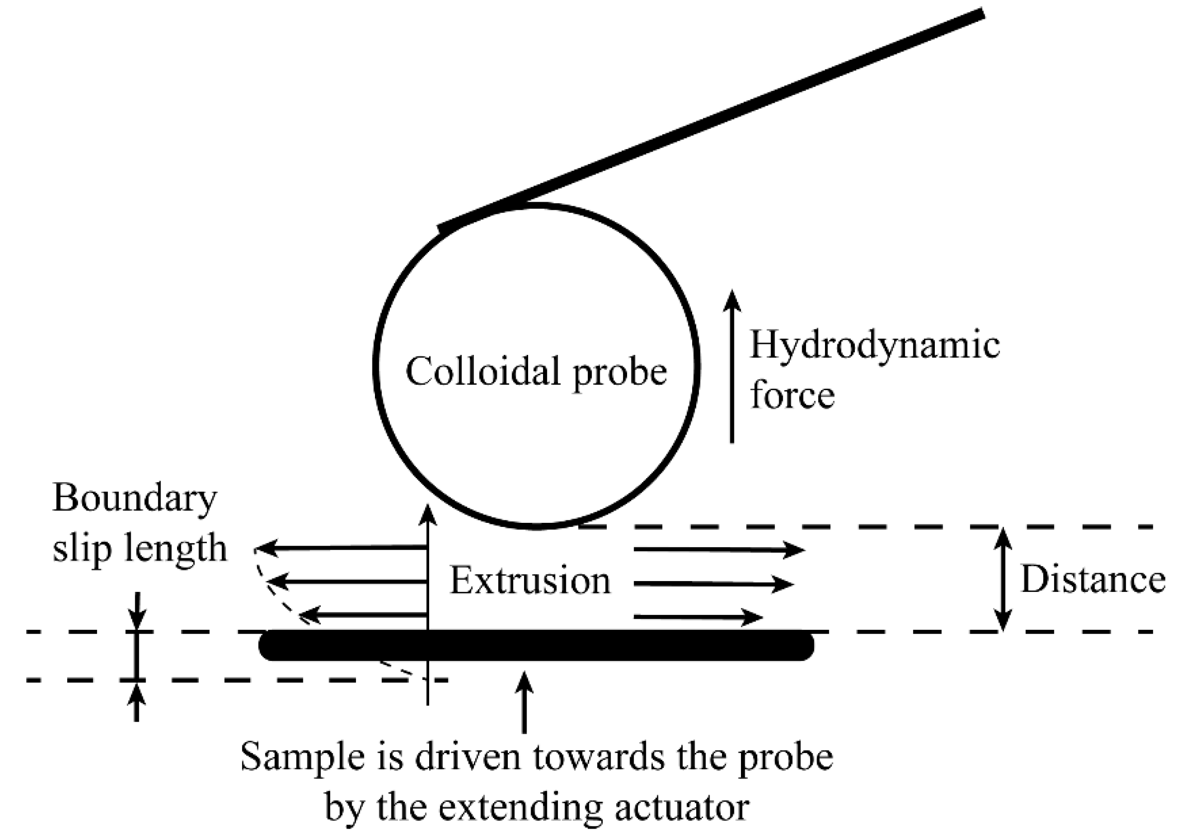
2. Measurement Model and Application Scope

When the boundary slip is measured using the CP-AFM method, according to the measurement model shown in Figure 1, a colloidal probe will be driven towards the flat solid surface immersed in fluid, and then the deflection of the probe induced by the interaction between the probe and the surface in the fluid will be recorded as laser feedback signal offset on the PSD. The interaction between the probe and the surface is mainly hydrodynamic force, which can be affected by the boundary slip. Note here, if there are colloidal particles close to the substrate, the interaction between the probe and the surface will be significantly affected [27,28]. Here, we only focused on the situation for pure liquid, which means there should be no colloidal particles close to the surfaces.

The measuring principle is shown in Figure 1. When the surface is an ideally smooth plane while the sphere is also smooth, the relationship between the hydrodynamic force on the sphere and the separation distance is shown as [15,29]:

$$F_H=f^{*}\frac{6\pi \mu R^2}{D}V$$

(1)

where R is the radius of the sphere, V is the velocity, F_H is hydrodynamic force, $\mu$ is liquid viscosity and D is separation distance between the colloidal probe and the solid surface.

$f^{*}$ is the correction coefficient associated with the existence of boundary slip. The sphere and the ideal plane fulfill no-slip boundary condition when $f^{*}=1$; and, when the ideal plane is subject to a slip length of b while the sphere has no slip, the correction factor $f^{*}$ is expressed as [15,29]:

$$f^{*}=\frac{1}{4}\left\{1+\frac{6D}{4b}\left[(1+\frac{D}{4b})\ln (1+\frac{4b}{D})-1\right]\right\}$$

(2)

Additionally, when slip length of both the sphere and ideal plane is b, the correction factor is defined as [15,29]

$$f^{*}=\frac{D}{3b}\left[(1+\frac{D}{6b})\ln (1+\frac{D}{6b})-1\right]$$

(3)

The measurement should be based on this theoretical model, thus three important demands for the measurement method are proposed as follows:

1. Smooth borosilicate glass sphere should be used for the colloidal probe, which is widely considered fulfilling no-slip boundary condition [13,16,17,18].

2. The measuring surface of the sample is required to be flat and smooth, as obvious errors will occur on the surface with large roughness and curvature. Thus, surface roughness should meet: b >> R_z.

3. The measurement is localized since it based on point-contact model. In other words, the surface of sample is required to be homogenic, and several points should be taken on the measured surface to obtain the average value.

When separation distance is far greater than the slip length (D >> b), the relationship between the hydrodynamic force and condition of solid–liquid interface boundary slip can be simplified as:

$$\frac{V}{F_H}=\frac{1}{6\pi \mu R^2}(D+b)$$

(4)

It can be defined from Equation (4) that the relationship between V/F_H and the separation distance is linear. Thus, the experimental results of V/F_H can be fitted and the linear regression line-intercept on the separation distance D is boundary slip length b. The advantage of this method is that the calculation of boundary slip b is no longer dependent on the parameters including radius of the sphere R and fluid viscosity μ. Eventually, the linearity of the curve needs to be checked, to see whether different data fitting segments would result in similar boundary slip length with little deviation.

3. Standard Process of Measuring Boundary Slip

3.1. Experimental Process

3.1.1. Sample and Condition

Deionized water made by Milli-QA10 system, a polished wafer covered by silicon dioxide (direction 1-0-0), borosilicate glass spheres (BSGMS, Cospheric LLC, Santa Barbara, USA), AFM probe (ORC-8, SNL, Bruker, Santa Barbara, USA), AFM (Dimension 3000, Bruker, Santa Barbara, USA), epoxy resin (Ergo 7200, Kisling, Zurich, Switzerland) and drop volume meter (MAIST, Vision, Beijing, China) were used in the experiment. The nominal spring constant of ORC8-10 was 0.1 N/m, the resonant frequency was 19 kHz, typical width and length were 40 μm and 200 μm, and the rectangular cantilever was coated by reflective gold. Although there were tips (around 3μm high) on the cantilever, they were covered when the spheres were stuck to the end of cantilever.

During the experiments, to realize the measurement of liquid environments, a colloidal probe was installed in a poly vinyl chloride liquid holder (DTFML-DD, Bruker, Santa Barbara, USA). In the holder, there were piezoelectric ceramics components, which drove the colloid probe movement in the liquid environment. Before measurement, a certain volume of liquid was dropped in between the liquid holder and the sample. The liquid formed a half-moon-shaped droplet. The liquid holder made volume of droplet greater as well as prevented pollution caused by evaporation.

Experiments were operated on the hydrophilic silica surface. First, the silicon wafers were placed into configured Piranha solution (H₂O₂ and H₂SO₄ 3:1 mix) for about 30 min, and then a large amount of ionic solution was used to clean the wafer. Next, acetone and ethanol were used for ultrasonic cleaning of silicon wafers for at least 5 min each, which were then dried with clean compressed air.

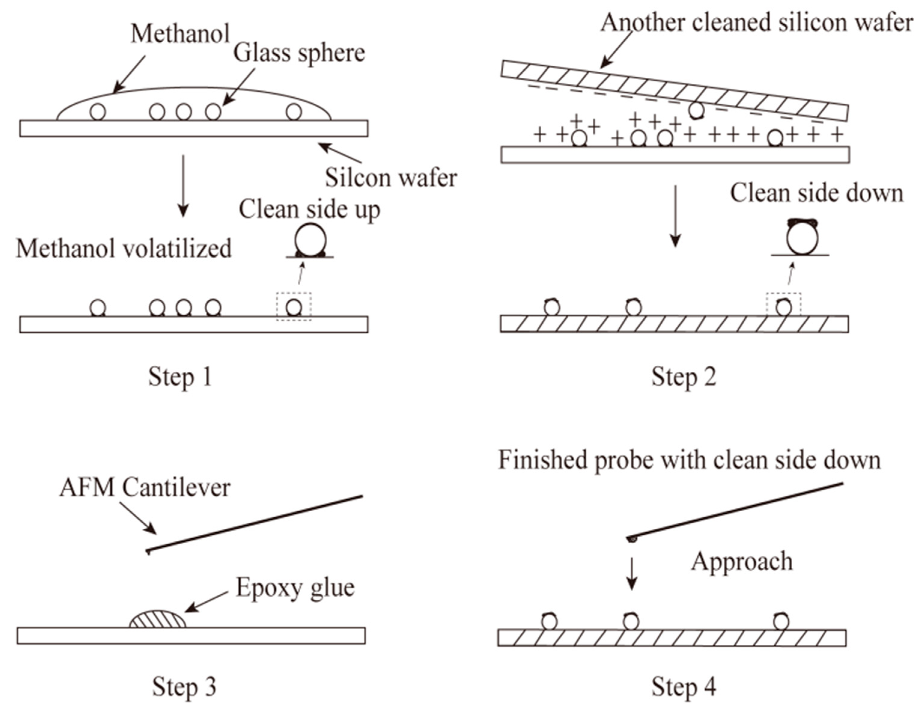
3.1.2. Probe Preparation

The preparation of the colloid probe was to make different radii borosilicate glass spheres (radius: 26–34 µm) stick to the end of AFM probe cantilever. It was necessary to ensure that probe surface was smooth and free from impurities when measuring. First, several borosilicate glass spheres were soaked in acetone solution and ultrasonically cleaned for 10 min, and then the acetone soaking solution was filtered out. A methanol solution was used to soak and filter repeatedly to remove residual acetone. Finally, the mixture of methanol solution and glass spheres was obtained. The process of probe preparation is shown in Figure 2, showing the six steps to prepare the colloidal probe.

The mixture of sphere and methanol was dropped on a silicon wafer. After the alcohol completely was completely volatized as the cleaner, the left side of the spheres faced up, as shown in Step 1. Electrostatic guns were used to “Jet” cations onto the silicon wafer, which contained spheres and “Jet” anions on another clean wafer. Then, the clean wafer was placed close to the wafer containing spheres, face to face. After the two wafers were separated, some spheres were stuck to the surface of the clean silicon wafer as the cleaning side face down, as shown in Step 2. Through a microscope, the tip of the probe was made to touch epoxy glue (Araldite, Bostik, Coubert) placed on the microslide gently, as shown in Step 3. When the probe touched the epoxy glue, it was lifted away from the glue to minimize the glue amount on the probe, as too much glue may contaminate the working side of the sphere. The clean wafer containing spheres was placed under the microscope, and the sphere was stuck in the center of the probe tip so that the sphere’s cleaning side faced down as the working side of the colloid probe, as shown in Step 4.

The working surface of the sphere was clean because the probe was prepared in a clean environment. Because of the gravity force and electrostatic adsorption, the dust and particles were moved to the non-working surface of the sphere or silicon wafer. As a result, the probe preparation method improved the experimental success rate and data validation.

3.1.3. AFM Scan Mode

AFM scan mode consists of contact mode and tapping mode. When using AFM, it is necessary to choose suitable scan mode in different conditions. We chose AFM contact mode to measure boundary slip in this study. Although the tapping mode is more sensitive to smaller force and it can improve the accuracy of boundary slip measurements, the model does not consider that the higher-order vibrations influence the measurement accuracy. Especially when the slip length is small, the tapping mode will produce errors because the high-order vibration cannot be ignored when closer to the surface. That is, the tapping mode is applicable to super hydrophobic surfaces whose boundary slip is more obvious. As for the hydrophobic surface whose slip length is smaller, it is better to use the contact mode.

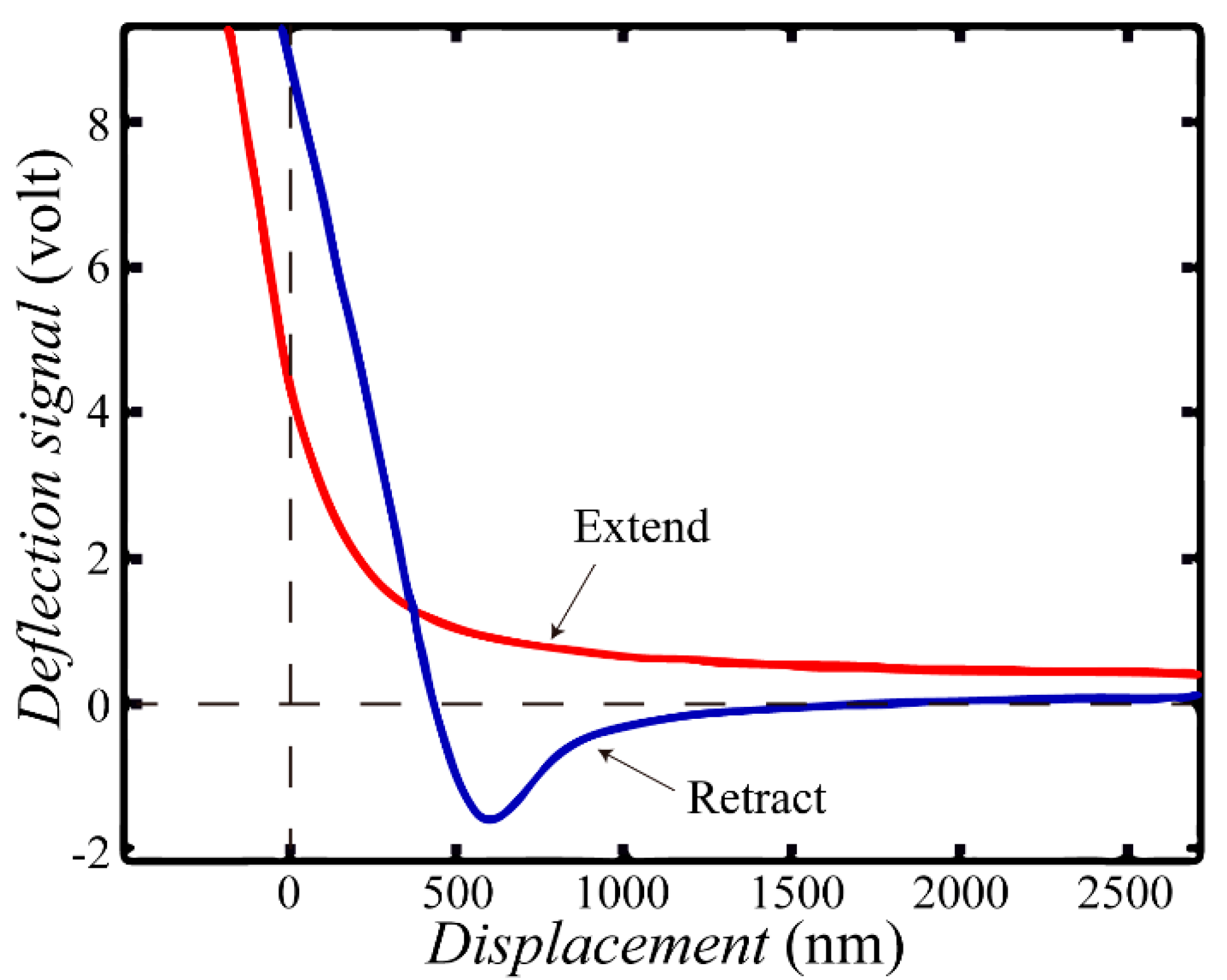
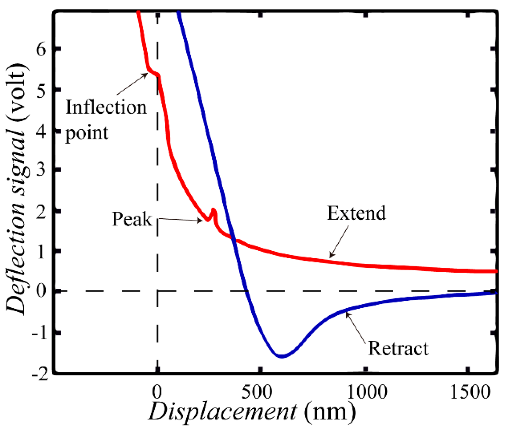
3.2. Data Processing

According to Equation (1), the data processing is to obtain the relationship between the hydrodynamic force and separation distance. The linear relationship between $V/F_H$ and separation distance can be calculated using Equation (4), based on which we study the boundary slip more intuitively.

The original data consisted of extend and retract curves, which recorded data when the z-axis actuator of the AFM extended and retracted, resulting in the sphere approaching and moving away from the surface. As shown in Figure 3, the latter presented negative peaks due to adhesion. The ordinate of the two curves is the voltage signal, which is the feedback based on photodiode detection system collecting cantilever deflection signals. The abscissa is the driving displacement, obtained by ultimate driving displacement minus the real-time driving displacement. A smaller value of the abscissa indicates that the probe moved closer to the surface.

There are two linear regions on each curve in Figure 3. When farther away from the surface, the probe was not affected by hydrodynamic force. Thus, both curves are almost horizontal lines, as shown by the linear area on the right side of Figure 3. As the value of driving displacement decreased to a certain extent, the probe contacted the surface of the sample. From this moment on, the probe deflection changed linearly with the driving displacement, as shown by the left area of Figure 3.

Although these two linear regions had nothing to do with the hydrodynamic force, they were used to finalize the data calibration, which directly affected the slip measurement results. For example, to remove the virtual deflection of AFM, i.e., the “fake” deflection when the z-actuator extended or retracted, even though there was no force applied on the probe [1]. Thus, before data processing, curve verification should be carried out as follows.

1. To facilitate the follow-up process of virtual deflection removing, as a matter of experience, the right-side length of the linear curve must be at least 500 nm based on the width of fitting area.

2. To accurately get the position where probe and the surface of the sample contacted each other, the left side of the curve must have good linearity and range. Thus, the zero-point offset should be avoided.

3. During the measurement, if the probe contacts roughness peaks or contaminants on the sample surface, there will be some inflection points on the curv, which will result in deviations. Thus, before the data processing, a curve with good smoothness should be selected.

For example, when obtaining the curve of the original data, as shown in Figure 4, inflection points and peaks caused uncontrollable bias to linear fit and made it difficult to accurately determine the position where probe and the surface of the sample contacted each other (the coordinate origin). In addition, due to the lack of information on the remote side, we could not remove the virtual deflection of the cantilever, which affected the processing of the subsequent linear fitting of the curve.

(1) Pre-treatment of the curves

Extend and retract curves are theoretically coincident on the left side. However, there were deviations of contact ratio between two original data curves due to the piezoelectric ceramic. Thus, the curves in Figure 3 had to be shifted closer and their coordinates were normalized. The result is shown in Figure 5. In most cases, the extend and retract curves are not coincide with each other at the liner part on the left because of the return error of AFM.

(2) Remove the virtual deflection

During the process of application of colloid probe technology, virtual deflection can make a large impact on measurement of hydrodynamic resistance. The virtual deflection increases as the separation distance between the probe and surface increases, which impacts the hydrodynamic resistance signal. Honig and Ducker [1] found that there is relative movement between the cantilever and the detector because of the piezoelectric ceramic. Thus, even without force, a certain amount of virtual deflection is generated. Thus, when measuring, the impact of this resistance should be excluded in the process. Zhu [15] reported that the pressure produced by the piezoelectric ceramic transducer generates a vertical elastic deformation, resulting in a virtual deflection. Their research indicated that the virtual deflection can be removed from the measuring process by subtracting the same slope’s linear part from the curve.

The extend curve is denoted as $De{f}_{ex}$, while the retract curve as $De{f}_{re}$. Then, the average curve of extend and retract curves can be calculated as:

$$De{f}_{average}=(De{f}_{ex}+De{f}_{re})/2$$

(5)

The remote linear portion of the average curve can be fitted linearly. Denoting the fitting curve as $De{f}_{average}^{\prime }$, the corrected extend curve can be obtained as:

$$De{f_{ex}}^{corrected}=De{f}_{ex}-De{f}_{average}^{\prime }$$

(6)

The corrected extend curve no longer had the extra slope of the curve caused by deflection of the instrument, as shown in Figure 6b.

The extend curve without virtual deflection is shown in Figure 7. The ordinate of the curve is the probe deflection measured in volts, and the abscissa is still the driving displacement.

(3) Transform of the abscissa to separation distance

After the steps above, the abscissa still did not represent the position of the surface. It was necessary to transform the abscissa (driving displacement) into the separation distance, and remove the instrument sensitivity so that the ordinate measured in volts could be transformed into the probe deflection in nm. There are several methods to calibrate the deflection [30,31,32]; here, the defection of the cantilever was obtained by the following process:

The linear region on the left was fit to obtain the intercept m and the slope of the linear part $k_i$. As noted above, the linear part on the left was where the hard contact occurred, so the change of the deflection should be equal to the change of the driving displacement. Thus, -$k_i$ is the cantilever sensitivity. The curve was divided by -$k_i$ to transform the ordinate into nanoprobe deflection. The curve is denoted as $De{f_{ex}}^{nm}$.

The origin point of the abscissa should be located at the contact position of probe and surface to make the abscissa associated with surface. It was necessary to shift the original abscissa, that is, subtract m from the original abscissa to obtain the new abscissa defined as Displacement, which is the driving position. The relationship among driving position, deflection of the probe and Distance (Distance is separation distance between the probe and surface simplified as D) is:

D = Displacement + Deflection

(7)

The separation distance (D) can be obtained based on Equation (7).

The relationship between separation distance and deflection of the probe is shown in Figure 8. After this procedure, the abscissa is the separation distance and ordinate is the deflection of the probe.

To confirm the validation of the deflection calibration, the data shown in Figure 8 were checked. When the sphere contacted the surface, the separation distance should be 0 nm, the data with high deflection value (in Figure 8, for example, the checking range is above 120 nm) should always be close to the deflection axis (D = 0 nm), and the error should smaller than 5 nm.

(4) Calculation of the probe spring constant

After obtaining the corrected probe deflections, the spring constant of the probe was calculated to obtain the total force on the probe.

As a colloidal probe in deionized water at a certain speed approaching the hydrophilic surface in non-slip condition, the deflection of cantilever can be expressed as [29]:

$$Def=\frac{F_H}{k}=\frac{6\pi \mu R^2}{kD}V$$

(8)

where V is the approximation rate between the sphere and sample surface, and k is spring constant of the colloid probe.

In fact, many studies present methods to calibrate the spring constant of the probe [33,34,35]. However, according to Equation (4), the slip length b is the linear regression line-intercept. As a scale factor, the spring constant does not affect b. Thus, it was not necessary to use the most accuracy way to obtain the spring constant. Thus, the spring constant of the colloid probe combined with the calibration of the cantilever deflection was obtained by the fitting method. The AFM colloidal probe approached a smooth flat hydrophilic surface in non-slip condition with a certain velocity, and then the deflection of the probe was measured. Finally, the deflection value of $k/6\pi \mu R^2$ was obtained using Equation (8). Then, the spring constant was calculated with the known values of $\mu$ and R (the sphere radius R could be measured by the light microscope).

For example, the probe was driven approaching a cleaned silicon wafer, which was assumed to be in non-slip condition with a velocity of 77 μm/s in deionized water. With such velocity, the electrostatic force was far less than the hydrodynamic force on the sphere. Then, the curve in the range of 1000–5000 nm was fitted to further reduce the effect of electrostatic force and van der Waals force. During the experiment, the radius of sphere was measured to be 29.3 μm, and the viscosity of deionized water in room temperature was $9.8\times {10}^{-4}\mathrm{kg}/\mathrm{m}\cdot \mathrm{s}$ [36]. The value of $k/6\pi \mu R^2$ fitted as 19 $\mathrm{nm}\cdot \mathrm{s}$, and the value of k was calculated as 0.3 N/m.

After obtaining the spring constant, the deflection was transformed into force on the probe. Then, the relationship between total force of the probe and separation was obtained, as shown in Figure 9.

(5) The treatment of electrostatic force, van der Waals force and Stokes force

When the probe approached the solid surface in the liquid, the force acting on the probe included electrostatic force F_E, van der Waals force F_van, Stokes F_S and hydrodynamic force F_H: F_total = F_E + F_van + F_S + F_H. Thus, to obtain the hydrodynamic force acting on the AFM colloidal probe, it was necessary to exclude the influence of van der Waals force, electrostatic force and Stokes force.

There are two methods for measuring electrostatic force: double-speed and low-speed methods. Hydrodynamic force acting on the colloidal probe (F_H) can be expressed as Equation (1), where hydrodynamic force is proportional to the velocity of the probe while electrostatic force does not influence the velocity of the probe. The double-speed method uses two different speeds for the probe approaching the surface. The low-speed method is based on the principle that, when the speed is low enough, hydrodynamic force is much smaller than electrostatic force, thus the former can be ignored. In this study, the low-speed method was used to measure the electrostatic force, and the driving speed of colloidal probe was chosen as 0.22 µm/s.

The van der Waals force between the sphere and flat can be expressed as [37,38]:

$$F_{van}=-\frac{\mathrm{A}R}{6D^2}$$

(9)

where A is Hamaker constant, R is radius of sphere and D is the separation distance.

When ignoring hydrodynamic force, the experimental data measured by AFM minus the van der Waals force is the electrostatic force. Since the slip length was calculated based on Equation (4) with fitting range as D ≥ 100 nm, and this distance was much larger than the scope of van der Waals force (0.5 nm), the van der Waals force can be ignored.

Since the cantilever always stayed away from solid surface (the distance was greater than or equal to the diameter of the sphere; in this example, the closest distance was 58.6 μm), the Stokes force on cantilever was not affected by the separation distance. It can be expressed as [18]:

$$F_S=-6\pi \eta l\dot{z}$$

(10)

where F_S is Stokes force, l is effective length of the cantilever and $\dot{z}$ is drive speed of piezoelectric ceramics.

As the Stokes force was obtained by fitting method, the parameters in Equation (10) were not measured.

When the sphere was moving far away from the surface, the force acting on the probe consisted of hydrodynamic force and Stokes force.

Based on Equation (1), hydrodynamic force is a function of separation distance, denoted as $f(D)$. Based on Equation (10), Stokes force was not affected by separation distance, thus the force acting on the probe can be expressed as:

$$F=F_H+F_S=f(D)+F_S=f^{*}\frac{6\pi \mu R^2}{kD}V+F_S$$

(11)

When the sphere was moving far away from the surface, V can be considered as constant and the Stokes force is also constant. Then, the force on the sphere can be expressed as follows, where C is a constant:

$$F=\frac{\mathrm{C}}{D}+F_S$$

(12)

Then, the Stokes force can be obtained by fitting the curve with Equation (12).

Finally, the influences including electrostatic force and Stokes force can be removed from the curve.

(6) Access to slip length

It should be noted that the driving velocity was not equal to approaching velocity due to the force on the sphere. As a result, the approaching velocity was obtained from the experimental data.

The relative value of time for each data point was obtained, and then the approaching velocity of the sphere was obtained by taking the derivative of separation distance of each data point. Finally, the curve of V/F_H was obtained, as shown in Figure 10. Eventually, b was obtained by fitting the certain distance of the curve. The slip length was the intersection coordinate value of the horizontal axis and curve. The two different curves in Figure 10 are the results of boundary slip measurements on two kinds of surfaces: surfaces of octadecyltrichlorosilane (OTS) and mica. The former is a hydrophobic surface, on which nanobubbles may exist [39,40] that lead to a finite slip length, while the latter is a hydrophilic surface in non-slip condition. Their original data were so similar to the data in Figure 3 that the slip length could only be calculated using the data in Figure 10, which were processed.

3.3. Roughness Correction of the Results

As mentioned above, the method in this study is only applicable to boundary slip length measurements on smooth and flat surfaces whose roughness meets b >> R_z. However, the ideal smooth surface does not actually exist. As a result, the roughness will influence the measuring result.

Thus, the data processing contained the method to correct the effects of roughness [23,26]. The majority of surfaces can be corrected by $B_{eff}=b-R_z$. As for some special surfaces, the reference surface position needs to be determined first. For two-dimensional sawtooth wave model, the reference surface height is $\frac{1}{2}{R}_z$ The correction methods of this model is $b_{eff}=b-R_z+\frac{1}{2}{R}_z$. For three-dimensional cone model, the reference surface height is $\frac{1}{4}{R}_z$. The correction methods of this model is $b_{eff}=b-R_z+\frac{1}{4}{R}_z$.

If the surface is almost ideal smooth, this step can be ignored.

4. Conclusions

Based on the model of measuring boundary slip by AFM in contact mode, this study developed a standard experimental procedure for the slip including data processing. The factors that can influence the measurements were analyzed and methods developed to minimize the effects, which include the effect of electrostatic force and Stokes force as well as the virtual deflection induced by relative motion between the detector and cantilever on the final result. Finally, the curve of V/F_H was obtained, based on which, the boundary slip was easily obtained. The developed standard procedure is general and practical for the measurement of boundary slip.

References

1. Honig, C.D.F.; Ducker, W.A. Thin film lubrication for large colloidal particles: Experimental test of the no-slip boundary condition. J. Phys. Chem C 2007, 111, 16300–16312. [Google Scholar] [CrossRef]
2. Nosonovsky, M.; Bhushan, B. Multiscale Dissipative Mechanisms and Hierarchical Surfaces: Friction, Superhydrophobicity, and Biomimetics; Springer: Heidelberg, Germany, 2008. [Google Scholar]
3. Bhushan, B. Springer Handbook of Nanotechnology, 3rd ed.; Springer: Heidelberg, Germany, 2010. [Google Scholar] [CrossRef]
4. Vinogradova, O.I. Slippage of water over hydrophobic surfaces. Int. J. Miner. Process. 1999, 56, 31–60. [Google Scholar] [CrossRef]
5. Jing, D.; Pan, Y. Electroviscous effect and convective heat transfer of pressure-driven flow through microtubes with surface charge-dependent slip. Int. J. Heat Mass Transf. 2016, 101, 648–655. [Google Scholar] [CrossRef]
6. Jing, D.; Pan, Y.; Wang, X. Joule heating, viscous dissipation and convective heat transfer of pressure-driven flow in a microchannel with surface charge-dependent slip. Int. J. Heat Mass Transf. 2017, 108, 1305–1313. [Google Scholar] [CrossRef]
7. Baudry, J.; Charlaix, E.; Tonck, A.; Mazuyer, D. Experimental evidence for a large slip effect at a nonwetting fluid-solid interface. Langmuir 2001, 17, 5232–5236. [Google Scholar] [CrossRef]
8. Cottin-Bizonne, C.; Cross, B.; Steinberger, A.; Charlaix, E. Boundary slip on smooth hydrophobic surfaces: Intrinsic effects and possible artifacts. Phys. Rev. Lett. 2005, 94, 056102. [Google Scholar] [CrossRef]
9. Xue, Y.H.; Wu, Y.; Pei, X.W.; Duan, H.L.; Xue, Q.J.; Zhou, F. How solid-liquid adhesive property regulates liquid slippage on solid surfaces? Langmuir 2015, 31, 226–232. [Google Scholar] [CrossRef] [PubMed]
10. Tretheway, D.C.; Meinhart, C.D. Apparent fluid slip at hydrophobic microchannel walls. Phys. Fluids 2002, 14, L9–L12. [Google Scholar] [CrossRef]
11. Joseph, P.; Tabeling, P. Direct measurement of the apparent slip length. Phys. Rev. E 2005, 71, 035303. [Google Scholar] [CrossRef]
12. VCraig, S.J.; Neto, C.; Williams, D.R.M. Shear-dependent boundary slip in an aqueous newtonian liquid. Phys. Rev. Lett. 2001, 87, 054504. [Google Scholar]
13. Wang, Y.L.; Bhushan, B.; Maali, A. Atomic force microscopy measurement of boundary slip on hydrophilic, hydrophobic, and superhydrophobic surfaces. J. Vac. Sci. Technol. A 2009, 27, 754–760. [Google Scholar] [CrossRef]
14. Maali, A.; Pan, Y.; Bhushan, B.; Charlaix, E. Hydrodynamic drag-force measurement and slip length on microstructured surfaces. Phys. Rev. E 2012, 85, 066310. [Google Scholar] [CrossRef] [PubMed]
15. Zhu, L.W.; Attard, P.; Neto, C. Reliable measurements of boundary slip by colloid probe atomic force microscopy. II. Hydrodynamic force measurements. Langmuir 2011, 27, 6712–6719. [Google Scholar] [CrossRef]
16. Pan, Y.L.; Bhushan, B.; Zhao, X.Z. The study of surface wetting, nanobubbles and boundary slip with an applied voltage: A review. Beilstein J. Nanotechnol. 2014, 5, 1042–1065. [Google Scholar] [CrossRef] [Green Version]
17. Pan, Y.L.; Bhushan, B. Role of surface charge on boundary slip in fluid flow. J. Colloid Interface Sci. 2013, 392, 117–121. [Google Scholar] [CrossRef]
18. Jing, D.; Bhushan, B. The coupling of surface charge and boundary slip at the solid–liquid interface and their combined effect on fluid drag: A review. J. Colloid Interface Sci. 2015, 454, 152–179. [Google Scholar] [CrossRef]
19. Bowles, A.P.; Ducker, W.A. Flow of water adjacent to smooth hydrophobic solids. J. Phys. Chem C 2013, 117, 14007–14013. [Google Scholar] [CrossRef]
20. Henry, C.L.; Craig, V.S.J. Measurement of no-slip and slip boundary conditions in confined newtonian fluids using atomic force microscopy. Phys. Chem. Chem. Phys. 2009, 11, 9514–9521. [Google Scholar] [CrossRef] [PubMed]
21. Rodrigues, T.S.; Butt, H.J.; Bonaccurso, E. Influence of the spring constant of cantilevers on hydrodynamic force measurements by the colloidal probe technique. Colloids Surf. A-Physicochem. Eng. Asp. 2010, 354, 72–80. [Google Scholar] [CrossRef]
22. Honig, C.D.F.; Ducker, W.A. No-slip hydrodynamic boundary condition for hydrophilic particles. Phys. Rev. Lett. 2007, 98, 028305. [Google Scholar] [CrossRef] [PubMed]
23. Guriyanova, S.; Semin, B.; Rodrigues, T.S.; Butt, H.J.; Bonaccurso, E. Hydrodynamic drainage force in a highly confined geometry: Role of surface roughness on different length scales. Microfluid. Nanofluidics 2010, 8, 653–663. [Google Scholar] [CrossRef]
24. Bonaccurso, E.; Butt, H.J.; Craig, V.S.J. Surface roughness and hydrodynamic boundary slip of a newtonian fluid in a completely wetting system. Phys. Rev. Lett. 2003, 90, 144501. [Google Scholar] [CrossRef] [PubMed]
25. Vinogradova, O.I.; Yakubov, G.E. Surface roughness and hydrodynamic boundary conditions. Phys. Rev. E 2006, 73, 045302. [Google Scholar] [CrossRef]
26. Pan, Y.; Jing, D.; Zhao, X. Effect of Surface Roughness on the Measurement of Boundary Slip Based on Atomic Force Microscope. Sci. Adv. Mater. 2017, 9, 122–127. [Google Scholar] [CrossRef]
27. Amano, K.I.; Iwaki, M.; Hashimoto, K.; Fukami, K.; Nishi, N.; Takahashi, O.; Sakka, T. Number Density Distribution of Small Particles around a Large Particle: Structural Analysis of a Colloidal Suspension. Langmuir 2016, 32, 11063–11070. [Google Scholar] [CrossRef] [PubMed]
28. Amano, K.I.; Ishihara, T.; Hashimoto, K.; Ishida, N.; Fukami, K.; Nishi, N.; Sakka, T. Stratification of Colloidal Particles on a Surface: Study by a Colloidal Probe Atomic Force Microscopy Combined with a Transform Theory. J. Phys. Chem. B 2018, 122, 4592–4599. [Google Scholar] [CrossRef]
29. Vinogradova, O.I. Drainage of a Thin Liquid-Film Confined between Hydrophobic Surfaces. Langmuir 1995, 11, 2213–2220. [Google Scholar] [CrossRef]
30. Slattery, A.D.; Blanch, A.J.; Quinton, J.S.; Gibson, C.T. Accurate measurement of atomic force microscope cantilever deflection excluding tip-surface contact with application to force calibration. Ultramicroscopy 2013, 131, 46–55. [Google Scholar] [CrossRef]
31. Sader, J.E.; Lu, J.; Mulvaney, P. Effect of cantilever geometry on the optical lever sensitivities and thermal noise method of the atomic force microscope. Rev. Sci. Instrum. 2014, 85, 113702. [Google Scholar] [CrossRef]
32. Higgins, M.J.; Proksch, R.; Sader, J.E.; Polcik, M.; Mc Endoo, S.; Cleveland, J.P.; Jarvis, S.P. Noninvasive determination of optical lever sensitivity in atomic force microscopy. Rev. Sci. Instrum. 2016, 77, 013701. [Google Scholar] [CrossRef]
33. Slattery, A.D.; Quinton, J.S.; Gibson, C.T. Atomic force microscope cantilever calibration using a focused ion beam. Nanotechnology 2012, 23, 285704. [Google Scholar] [CrossRef]
34. Slattery, A.D.; Blanch, A.J.; Quinton, J.S.; Gibson, C.T. Calibration of atomic force microscope cantilevers using standard and inverted static methods assisted by FIB-milled spatial markers. Nanotechnology 2013, 24, 015710. [Google Scholar] [CrossRef] [PubMed]
35. Sader, J.E.; Borgani, R.; Gibson, C.T.; Haviland, D.B.; Higgins, M.J.; Kilpatrick, J.I.; Lu, J.; Mulvaney, P.; Shearer, C.J.; Slattery, A.D.; et al. A virtual instrument to standardise the calibration of atomic force microscope cantilevers. Rev. Sci. Instrum. 2016, 87, 093711. [Google Scholar] [CrossRef] [Green Version]
36. Haynes, W.M. Handbook of Chemistry and Physics, 96th ed.; Academic Press: New York, NY, USA, 2015. [Google Scholar]
37. Attard, P.; Parker, J.L. Deformation and adhesion of elastic bodies in contact. Phys. Rev. A 1992, 46, 7959–7971. [Google Scholar] [CrossRef] [PubMed]
38. Zhu, L.; Attard, P.; Neto, C. Reliable measurements of boundary slip by colloid probe atomic force microscopy. I. Mathematical modeling. Langmuir 2011, 27, 6701–6711. [Google Scholar] [CrossRef]
39. Wang, Y.; Bhushan, B. Boundary slip and nanobubble study in micro/nanofluidics using atomic force microscopy. Soft Matter 2010, 6, 29. [Google Scholar] [CrossRef]
40. Ishida, N.; Inoue, T.; Miyahara, M.; Higashitani, K. Nano bubbles on a hydrophobic surface in water observed by tapping-mode atomic force microscopy. Langmuir 2000, 16, 6377. [Google Scholar] [CrossRef]
Figure 1. AFM (Atomic force microscope) contact mode measurement model and principle.
Applsci 09 01453 g001
Figure 2. The preparation principle of colloidal probe.
Applsci 09 01453 g002
Figure 3. The original data of process and return curve at a velocity of 77 μm/s.
Applsci 09 01453 g003
Figure 4. The original data curve unable to process.
Applsci 09 01453 g004
Figure 5. Curves close treatment.
Applsci 09 01453 g005
Figure 6. (a) Virtual deflection due to the relative motion of the detector; and (b) the deflection curve after removal of virtual deflection.
Applsci 09 01453 g006
Figure 7. Process curve after removing virtual deflection.
Applsci 09 01453 g007
Figure 8. The extend curve transformed such that the abscissa is the separation distance.
Applsci 09 01453 g008
Figure 9. Force–distance curve of probe.
Applsci 09 01453 g009
Figure 10. Boundary slip measurements on different surfaces: black, OTS; red, mica.
Applsci 09 01453 g010