On the Performance of Deep Reinforcement Learning-Based Anti-Jamming Method Confronting Intelligent Jammer

Abstract

With the development of access technologies and artificial intelligence, a deep reinforcement learning (DRL) algorithm is proposed into channel accessing and anti-jamming. Assuming the jamming modes are sweeping, comb, dynamic and statistic, the DRL-based method through training can almost perfectly avoid jamming signal and communicate successfully. Instead, in this paper, from the perspective of jammers, we investigate the performance of a DRL-based anti-jamming method. First of all, we design an intelligent jamming method based on reinforcement learning to combat the DRL-based user. Then, we theoretically analyze the condition when the DRL-based anti-jamming algorithm cannot converge, and provide the proof. Finally, in order to investigate the performance of DRL-based method, various scenarios where users with different communicating modes combat jammers with different jamming modes are compared. As the simulation results show, the theoretical analysis is verified, and the proposed RL-based jamming can effectively restrict the performance of DRL-based anti-jamming method.

1. Introduction

With the rapid development of wireless communications, the information security has attracted more and more attention. In sensitive areas such as airports [1] and electronic warfare-type battlefield [2], anti-jamming techniques are needed for against illegal jammers. With the development of artificial intelligence (AI) [3], communication devices are becoming increasingly intelligent [4]. Users are able to learn the jamming modes with the help of AI technologies, the probability of being jammed can be reduced by making the right decision, such as switching to idle communication frequencies [5] or adjusting the communication power [6].

The traditional jamming modes include sweeping jamming, comb jamming, and barrage jamming [7]. Due to the fixed jamming pattern, the traditional jamming can be easily avoided by the users. For example, sweeping jamming could be avoided by selecting communication time [8]. Comb jamming could be avoided by selecting communication frequency. For barrage jamming, as the range of the jammed frequencies grows bigger, the output power of the barrage jamming is reduced proportionally [9]. When the power of jamming is low, the jamming could be invalid by choosing the appropriate communication power [6]. The anti-jamming strategies based on the principle of statistics [10], game theory [11], and the other approaches [12,13] have excellent effects on reducing the probability of being jammed.

In order to improve the jamming effect, anti-jamming methods are needed to take into consideration when we design a jamming method. There are many kinds of anti-jamming methods [14,15,16], such as frequency hopping [14], fixed frequency with a greater communication power [15], direct sequence spread spectrum (DSSS) [16]. In [17], link-layer jamming and the corresponding anti-jamming methods are overviewed. Link-layer jamming can analyze the user’s Media Access Control (MAC) protocol parameters, and releases a high energy-efficiency jamming attack. In addition to the adversarial jamming, we can also utilize the cooperative jamming techniques to improve the physical-layer security [18]. In order to face the developing of anti-jamming, many researchers use optimization, game-theoretic or information theoretic principles to improve the jamming performance [19,20,21,22]. However, these methods require some prior information (the communications protocol, user’s transmission power, etc.) that is difficult to obtain in the actual environment. Other researchers solve the jamming problem with repeatedly interacting with the victim transmitter-receiver pair [23], combining optimization, game-theoretic theories and other theoretical tools. But these only take the situation that the user has a fixed strategy into consideration, or choose a strategy from a strategy set. It is difficult to design the efficient jamming strategy when facing an intelligent user that could change communication strategy by learning [24].

In [24], a dynamic spectrum access anti-jamming method based on a deep reinforcement learning (DRL) algorithm was designed. With a DRL algorithm, intelligent users can learn the jammer’s strategy by trail-and-error channel accessing process and obtain the optimal anti-jamming policy with no need of jammer’s information. As concluded in [24], even the space of spectral states is infinite, the powerful approximation capability of deep neural network can still converge to the optimal policy, and the success rate could get around $95\%$ against sweeping, comb and dynamic jamming, which performs much better than the traditional reinforcement learning algorithm.

The DRL-based anti-jamming method are powerful, but to the best of our knowledge, the efficient jamming approach against the DRL-based communication user has not been researched. What will happen when the jammer is also intelligent which can learn the communication mode of users and adjust its jamming strategy dynamically? Inspired by [25], in this paper, we investigate the performance of DRL-based anti-jamming method in face of different modes of jamming, including traditional jammers and intelligent jammer based on reinforcement learning (RL). RL [26,27] is an intelligent algorithm that gets feedback from the environment which does not need the priori information. Compare to DRL, an RL algorithm needs less calculation and fewer iterations to converge. In the wireless network, communication devices often access the spectrum for a short time, which only provide the jammers with a small amount of data. Due to this reason, we assume that the jammer adopts RL algorithm, instead of DRL.

In this paper, we design an RL-based jamming algorithm and investigate the performance of a DRL-based anti-jamming method. The implementation as well as the theoretical performance are discussed. Different from [28], we take a small possibility of random jamming as a way to against DRL-based user. We theoretically analyze the condition when the DRL-based anti-jamming algorithm does not converge and provide the process of proof. The main contributions are summarized as follows:

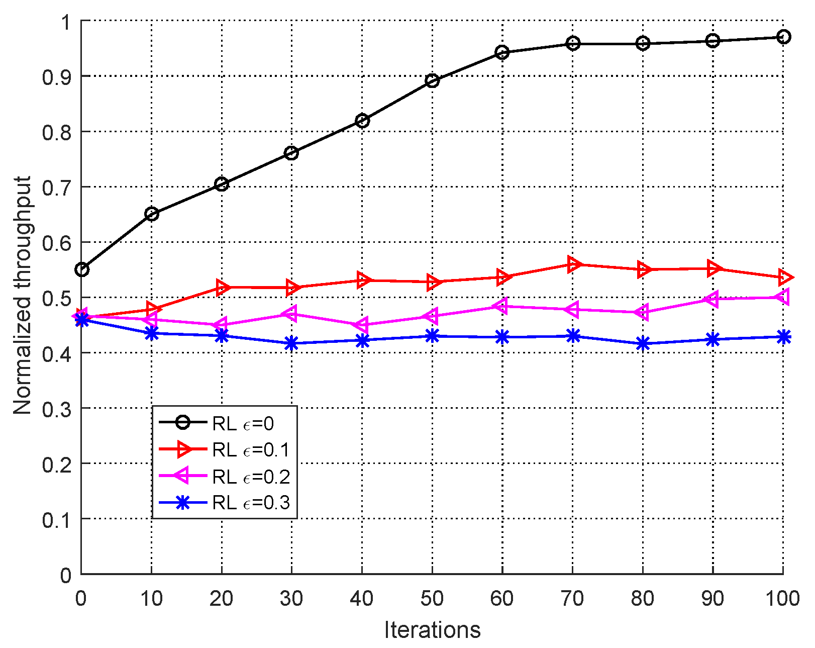
• We investigate the performance of DRL-based anti-jamming method in face of different jamming modes. Without the prior information of users, we designed an RL-based jamming algorithm to against the DRL algorithm, and the simulation results verify the effectiveness of the jamming method.
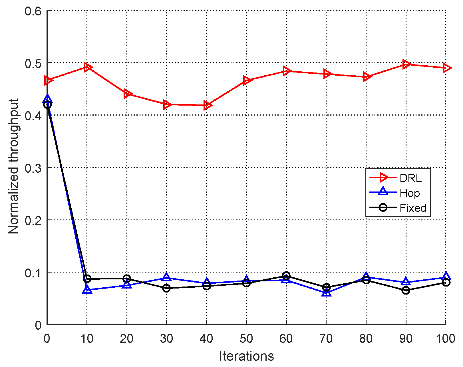
• We theoretically analyze the condition when the DRL-based algorithm cannot converge, and verified it by simulation.

We organize this paper as follows. Section 2 discusses system model. In Section 3, we present the RL-based jamming algorithm. The analysis of DRL algorithm is provided in Section 4, followed by the simulation results in Section 5. Concluding remarks of the paper are in Section 6.

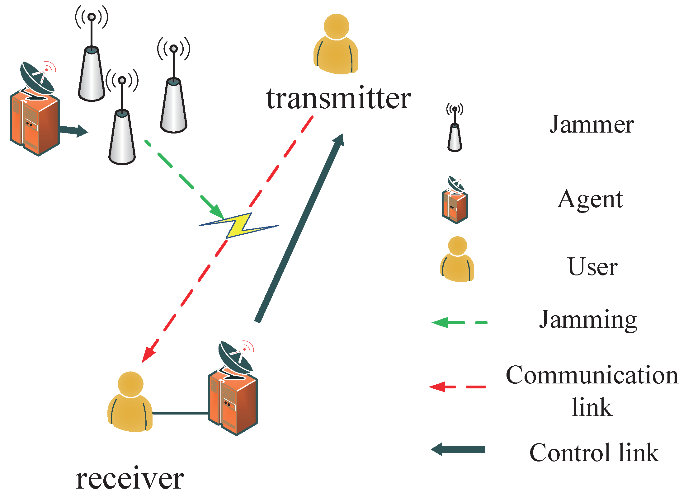
2. System Model and Problem Formulation

As shown in Figure 1, the system model consists of two users (a transmitter-receiver pair), two agents (one for the user, the other for jammer), which can sense the frequency spectrum by performing full-band detection every $t_s$ with step $\Delta f$. According to the sensing, agents guide the frequency choice of jammers or user respectively. The transmitter is equipped with one transmission radio interface that can communicate on one frequency band at one time. The communication frequency range of the transmitter is denoted by $B_u$, and transmission signal bandwidth is $b_u$. Channel selection set for transmitter is marked as ${\mathcal{A}}_u=\{a_1,a_2,\dots ,a_N\}$ ($\left|{\mathcal{A}}_u\right|=N$). The agent senses the whole communication band continuously and selects a communication channel over N ($N=\frac{B_b}{b_u}$) channels for transmitter through control link. The receiver is a full band receiver, it reports to the agent the quality of the received signal through control link or wire link.

For the jammer, we use $b_j$ to denote the jamming band for the jammer at one time, and a jammer can jam several frequency bands. The jamming frequency range is denoted by $B_j$, we set $B_j=B_u$. The number of the jammer’s decision set can be calculated as $M=\frac{B_j}{b_j}$. The action set of jammer can be denoted by ${\mathcal{A}}_j=\{a_1,a_2,\dots ,a_M\}$ ($\left|{\mathcal{A}}_j\right|=M$).

To simplify the analysis, we divide the continuous time into discrete time slots (have shown in Figure 3), and assume that both jammer and user consume the same time $\tau$ for making strategy and Assuming that the decision strategy of users and jammer remains unchanged during the time slot $\tau$.

Agent and Optimized Objective of Jammers

The agent of a jammer can sense the communication channels, analyzes the communication preference of user, and guide deployment of jamming through reliable control link or wire link. The signal-to-interference-plus-noise ratio (SINR) of the user’s receiver can be noted by

$$\beta \left(f_t,f_t^j\right)=\frac{g_u{p}_u}{{\int }_{f_t-b_u/2}^{f_t+b_u/2}\left\{n\left(f\right)+{\displaystyle \sum _{j=1}^n}{g}_j{J}_t^j\left(f-f_t^j\right)\right\}df},$$

(1)

where the center transmission frequency at time t is denoted by $f_t$. The parameter $b_u$ is the user transmission bandwidth. The transmitted power of a user is denoted by $p_u$, $n\left(f\right)$ is the power spectral density (PSD) of noise, $f_t^j$ denotes the selecting jamming center frequency by Jammer j at time t. PSD of one jamming band is denoted by $J\left(f\right)$, $g_j$ is the channel gain from jammer to the user’s receiver. Denoting the channel gain from user’s transmitter to the jammer as $g_u$. Set $\mu \left(f_t\right)$ as an indicator function for successful transmission as follows:

$$\mu (f_t,f_t^j)=\left\{\begin{array}{c}1,\beta (f_t,f_t^j)\ge {\beta }_{th}\hfill \\ 0,\beta (f_t,f_t^j)<{\beta }_{th}\hfill \end{array}\right.,$$

(2)

where ${\beta }_{th}$ is defined as the threshold of SINR. When the SINR is below the threshold, ${\beta }_{th}<\beta \left(f_t\right)$, the transmission is seen as failed. The aim of jammer is to minimize the target function:

$$\underset{f_t^j\in A_j}{min}\mathsf{\Lambda }=\sum _{t=0}^{\infty }{\gamma }^t\mu (f_t,f_t^j),$$

(3)

where $\gamma$ is the discount factor and $\gamma \in (0,1)$.

We set $u_{t,i}$ as discrete spectrum sample value $u_{t,i}=10log(\int {}_{i\Delta f_j}^{(i+1)\Delta f_j}{R}_j\left(f\right)df)$, $\Delta f_j$ is the resolution of spectrum analysis of jammer, and $R_j\left(f\right)$ is denoted by:

$$R_j\left(f\right)=g_{a}U(f-f_t)+\sum _{j=1}^J{g}_{a,j}{J}_t^j(f-f_t^j)+n\left(f\right),$$

(4)

where $g_a$ is the channel gain from user’s transmitter to the agent end, and $g_a,j$ is the channel gain from jammer to jammer’s agent end. With $u_{t,i}$, we can rebuild the spectrum at time t, find the user’s communication frequency, and denote as $u_{t,c}$. The total range of a jammer can jam at one time is $B_j^n={\displaystyle \sum _{i=1}^n}{b}_j^i$, $b_j^i$ is the jamming band for jammer i, note that the $B_u>B_j^n$.

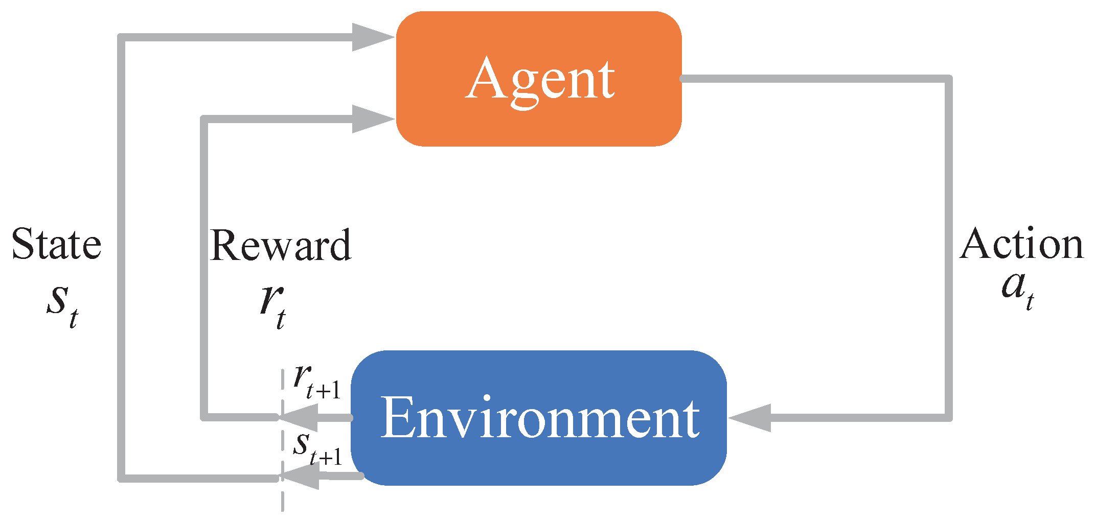
3. RL-Based Jamming Algorithm

The main task of RL is to adjust the strategy according to the feedback information obtained from the environment. In our case, the feedback is the jamming effect. By feedback, the algorithm improves the effectiveness of its decision strategy. Some researchers have applied RL to solve anti-jamming or jamming problems [29,30,31]. However, they assumed the strategy of the opponent is fixed or choosing strategy in a strategy set. The algorithm cannot apply well if the opponent is intelligent which can change the strategy through learning. We explain the essence of RL by four crucial elements, i.e., agent, state, action and reward [32].

• Agent: The agent is responsible for making decisions. It usually has the capability of sensing the environment and taking actions. In our case, the agent could sense the frequency spectrum and guides jammer to choose jamming band.
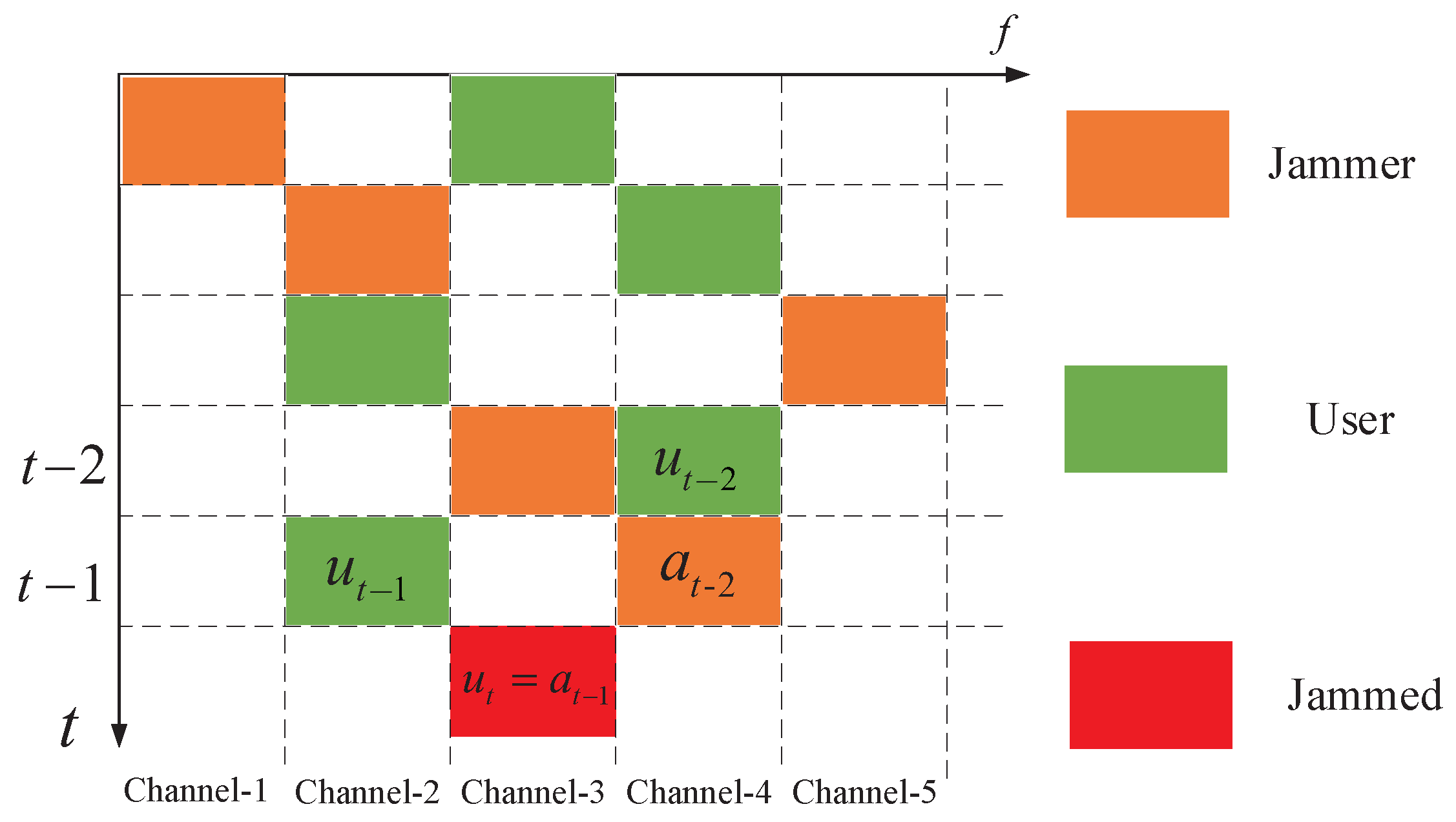
• State: Environment state for the corresponding action. In our case, the state is the frequency spectrum that agent senses.
• Action: All actions can be taken by the agent, or under the guidance of agent. In our case, action is to jam which frequency band.
• Reward: Feedback of the corresponding action in the environment. In our case, reward is the jamming effect.

Figure 2 shows the process of RL algorithm. Agent gets state $s_t$ at time t, makes the action $a_t$, gets the reward at time t, and use the reward $r_t$ to update its value function. Then, the agent repeats the process at time $t+1$.

3.1. Reward

With the setting of reward value, the intelligent agent can know which actions are effective in a given environment and which are not. When jamming successfully, reward R is 1. If not, R should be 0. Then the agent learns to make the more effective decision in the corresponding state. As shown in Figure 3, the horizontal axis represents frequency, and the longitudinal axis represents time. To simplify analysis, we set $b_u=b_j$. In this case, state is the user’s communication frequency band denoted as $u_t$ and action is the jamming frequency band denoted as $a_t$. Note decision $a_{t-1}$ is made at time $t-1$, and execute at time t. Figure 3 shows the relation of state and action, and R can be described as:

$$R=\left\{\begin{array}{c}1u_t=a_{t-1}\hfill \\ 0u_t\ne a_{t-1}\hfill \end{array}\right..$$

(5)

Note that, in an actual situation, it is hard for a jammer to judge if $u_t=a_{t-1}$. In order to know the jamming effect, the following methods can be used.

• Detect negative acknowledgement (NACK). In ref. [33], NACK is used as reward standard. If NACK is detected, we affirm $u_t=a_{t-1}$, $R=1$. Since the communication protocol of civil communication system is public, jammers can easily recognize NACK. However, in the actual situation, the users’ communication protocol is unknown. Auxiliary methods are needed for the jammers.
• Detect change of communication power. In ref. [34], the detection of increasing power is the sign of successful jamming. Many wireless communication devices are designed to increase power when it gets the interference or noise in the environment. Take a cell phone for example, when it can not communicate well to base station, a cell phone increases the communication power. By sensing the changing transmit power of users, we could affirm $u_t=a_{t-1}$, $R=1$.
• Detect users switching channels. In actual communication, switching channels usually requires negotiation between the transmitter and receiver and often consumes more energy. Due to the limited energy, users are more inclined to stay on the current channel to communication. Therefore, detecting the channel switching can also evaluate jammer effect.

3.2. Q-Learning

Q-learning is one of the most popular RL algorithms. The core updated formula [35] is given by:

$$\begin{array}{c}Q({u_t}_{-1},{a_t}_{-1})\leftarrow (1-\alpha )Q(u_{t-1},a_{t-1})+\alpha [R+\gamma \underset{a}{max}Q(u_t,a)],\hfill \end{array}$$

(6)

where $Q(u_{t-1},a_t)$ is the Q-value that evaluates the action $a_t$ at state $u_{t-1}$ (we set $\tau =1$), $\alpha \in (0,1)$ is the learning rate, R is the reward value.

In actual situation, a jammer could select n frequency bands to jam in decision set ${\mathcal{A}}_j$ (under guidance of agent). At time t, the decision is selected from $Q(u_{t,c},{\mathcal{A}}_j)$ (Q is a two-dimensional matrix), note ${\mathcal{A}}_{s,t}$ is the top n values selected from $Q(u_{t,c},{\mathcal{A}}_j)$ at time t, define this operation as $sort{\left[Q(u_{t,c},:)\right]}_{1:n}$. $R_{s,t}$ is the reward vector for corresponding actions. For example, if the actions ${\mathcal{A}}_{s,t}=\{a_{1,t},a_{2,t},a_{4,t}\}$ and if $a_{4,t}$, $R=1$, then $R_{s,t}=\left\{0,0,0,1,0,\dots ,0\right\},(\left|\mathcal{A}{}_j\right|=\left|R_{s,t}\right|=M)$. The update formula of jammer is as follows:

$$\begin{array}{c}Q(u_{t-1,c},{\mathcal{A}}_j)\leftarrow (1-\alpha )Q(u_{t-1,c},{\mathcal{A}}_j)+\alpha [R_{s,t}+\gamma Q(u_{t,c},{\mathcal{A}}_j)].\hfill \end{array}$$

(7)

The reinforcement learning jamming algorithm is repeated until any stop criterion is met (see Algorithm 1).

Algorithm 1 Reinforcement learning jamming algorithm (RLJA).

Initialize: Set learning rate $\alpha \in (0,1)$, discount rate $\gamma \in (0,1)$, $Q=0$, training time T, and probability of random action $\epsilon \in (0,1)$. The number of jamming frequency bands is n. for $t=1,2,\dots ,\infty$ do    Generate random value $\eta \in (0,1)$    if $t<T$ then        Agent chooses n action from ${\mathcal{A}}_j$ randomly ($a_t\in {\mathcal{A}}_j,\mathrm{P}(a_t=a)=\frac{1}{N}$, $N=\left|{\mathcal{A}}_j\right|$) gets reward,        update Q matrix:                 $Q(u_{t-1,c},{\mathcal{A}}_j)\leftarrow (1-\alpha )Q(u_{t-1,c},{\mathcal{A}}_j)+R_{s,t}+\alpha [R+\gamma Q(u_{t,c},{\mathcal{A}}_j)]$        if $\eta >\epsilon$ then         Agent choose action top n action, $sort{\left[Q(u_{t,c},:)\right]}_{1:n}$, ${\mathcal{A}}_{s,t}$, gets reward, updates Q matrix:                 $Q(u_{t-1,c},{\mathcal{A}}_j)\leftarrow (1-\alpha )Q(u_{t-1,c},{\mathcal{A}}_j)+R_{s,t}+\alpha [R+\gamma Q(u_{t,c},{\mathcal{A}}_j)]$        else         Agent chooses n action from ${\mathcal{A}}_j$ randomly, gets reward, updates Q matrix:                 $Q(u_{t-1,c},{\mathcal{A}}_j)\leftarrow (1-\alpha )Q(u_{t-1,c},{\mathcal{A}}_j)+R_{s,t}+\alpha [R+\gamma Q(u_{t,c},{\mathcal{A}}_j)]$        end if    else        Finish training    end if        Agent guides actions based on Q matrix end for

Theorem 1.

The jamming process of RL algorithm can converge with different ε under condition that the communication process is action replay process (ARP).

Proof. 

The proof is given in reference [35], which is divided into two parts. The first part explains what action-replay process (ARP) is. ARP is derived from a particular sequence of episodes observed in the real process, with a finite state space $\mathcal{S}$ and a finite action set $\mathcal{A}$. Second part proves that Q-learning algorithm can converge under condition that the process in real situation is ARP. Exploring conditions are not requirements to the proof, the iterations are. Since the jamming pattern without a random scheme in this case is ARP, iterations are enough. Therefore, the algorithm can converge. □

4. Theoretical Analysis of the Condition When DRL-Based Algorithm Does Not Converge

A DRL algorithm is a combination of a deep learning (DL) algorithm and reinforcement RL algorithm [36], it combines the perception ability of the DL algorithm and decision-making ability of RL. DL is used to extract environmental features from the complex environment, RL learns from features and optimizes itself by trial and error. Neural network is a nonlinear function approximator, through data training, to find the best-optimized function of a certain situation [37], which in this paper is to approximating the Q-function of RL. Motivated by [38], in this paper we prove that the DRL-based algorithm does not converge when facing with certain probability of random actions in steady-state dynamics. Then we verify our proof by simulation.

Theorem 2.

Anti-jamming process of DRL algorithm does not converge when facing with certain probability of random actions.

Proof. 

The following proof follows the lines given in [38]. To start with, note the anti-jamming process of DRL is a Markov process [24], first consider a Markov process with finite states $S=\{s_1,s_2,\dots ,s_n\}$. We assume that the cost of transition between states and the discount factor $\alpha \in (0,1)$. Let the function approximator be parametrized by a single scalar r.

$$\begin{array}{c}\tilde{J}\left(r\right)={(\tilde{J}(1,r),\tilde{J}(2,r),\dots ,\tilde{J}(n,r))}^T.\hfill \end{array}$$

(8)

We let the $\tilde{J}\left(0\right)$ be a nonzero vector that satisfies with $e^T\tilde{J}\left(0\right)=0$, where the $e=(\stackrel{n}{\overbrace{1,1,\dots ,1}}){}^T$. $\tilde{J}\left(r\right)$ is a unique solution to a linear differential equation [38]:

$$\begin{array}{c}\frac{d\tilde{J}}{dr}\left(r\right)=(Q+\sigma I)\tilde{J}\left(r\right)\hfill \end{array},$$

(9)

where I is a unit matrix of $n\times n$, and $\sigma$ is a tiny positive constant. Q matrix is average direction of the consequence of constant probability of random actions. It can be noted by:

$$\begin{array}{c}Q=\left[\begin{array}{cccc}{q}_{1,1}& q_{1,2}& \cdots & q_{1,n}\\ q_{2,1}& \cdots & \cdots & q_{2,n}\\ \cdots & \cdots & \cdots & \cdots \\ q_{n,1}& q_{n,2}& \cdots & q_{n,n}\end{array}\right].\hfill \end{array}$$

(10)

According to our definition of $\tilde{J}$, it is easy to know that all functions represented by $\tilde{J}$ can map to three-dimensional space $\{J\in {\Re }^3\left|e^{T}J=0\right.\}$. Set the Markov chain transition probability matrix is P, and can be denoted as:

$$\begin{array}{c}P=\left[\begin{array}{cccc}{p}_{1,1}& p_{1,2}& \cdots & p_{1,n}\\ p_{2,1}& \cdots & \cdots & \cdots \\ \cdots & \cdots & \cdots & \cdots \\ p_{n,1}& p_{n,2}^{}& \cdots & p_{n,n}\end{array}\right].\hfill \end{array}$$

(11)

Since the transition cost is set to 0, the $TD\left(0\right)$ operator [39] can be defined as $T^{\left(0\right)}=\alpha P$, for any $J\in {\Re }^3$, there is a certain angle $\theta$, and a scalar $\beta \in (0,1)$, for any r, $T^{\left(0\right)}\tilde{J}\left(r\right)$ is equal to the vector $\tilde{J}\left(r\right)$ extends $\beta$ and rotates the $\theta$ angle. Concretely, the update equation of $TD\left(0\right)$ can be addressed as:

$$\begin{array}{c}{r}_{t+1}=r_t+\gamma \frac{d\tilde{J}}{dr}\left(r\right)(\alpha \tilde{J}(i_{t+1},r_t)-\tilde{J}(i_t,r)),\hfill \end{array}$$

(12)

where the $i_t$ is the state at time t. The expectation of the update direction formula as follows:

$$\begin{array}{c}{\displaystyle \sum _{i=1}^n}\frac{d\tilde{J}}{dr}\left(\alpha {\displaystyle \sum _{i=1}^n}{p}_{i,j}\tilde{J}(j,r)-\tilde{J}(i,r)\right),\hfill \end{array}$$

(13)

where j is the state that the i state is going to visit next. $\alpha {\displaystyle \sum _{i=1}^n}{p}_{i,j}\tilde{J}(j,r)-\tilde{J}(i,r)$ is equivalent to $(\alpha P-I)\tilde{J}\left(r\right)$. From Equation (9), and as the $r_{t+1}-r_t$ becoming small enough, the algorithm update process can be approximated by another differential equation. The average direction is given by the parameter, the differential equation describing this process can be:

$$\begin{array}{c}\begin{array}{c}\frac{dr}{dt}={\left((Q+\sigma I)\tilde{J}\left(r\right)\right)}^T(\alpha P-I)\tilde{J}\left(r\right)\hfill \\ ={\tilde{J}}^T\left(r\right)(Q^T+\sigma I)(\alpha P-I)\tilde{J}\left(r\right),\hfill \end{array}\hfill \end{array}$$

(14)

for $\sigma =0$ (the process of neural network convergence is slow, then the $\sigma$ can approximate to 0), then we have:

$$\begin{array}{c}\frac{dr}{dt}={\tilde{J}}^T\left(r\right)Q^T(\alpha P-I)\tilde{J}\left(r\right)\hfill \\ =\alpha {\tilde{J}}^T\left(r\right)Q^{T}P\tilde{J}\left(r\right)\hfill \\ =\frac{\alpha }{2}{\tilde{J}}^T\left(r\right)(Q^{T}P+P^{T}Q)\tilde{J}\left(r\right),\hfill \end{array}$$

(15)

where the first equation comes from that ${\tilde{J}}^T\left(r\right)Q^T\tilde{J}\left(r\right)=0$, because the for large enough n, the $rank\left(Q^T\right)<n$. For example [38], $F=\left[\begin{array}{ccc}1& 1/2& 3/2\\ 3/2& 1& 1/2\\ 1/2& 3/2& 1\end{array}\right]$, then the $rank\left(F^T\right)=2$. For any r, note the Q matrix is average direction under influence constant probability of random actions. Because Q guides $\tilde{J}\left(r\right)$ to the direction of misconvergence, $\frac{Q·P}{∥Q∥∥P∥}=\theta >0$. Therefore, the $Q^{T}P+P^{T}Q$ is positive definite. With the setting of random actions, there exists a positive constant c that:

$$\begin{array}{c}\frac{dr}{dt}\ge c∥\tilde{J}\left(r\right)∥.\hfill \end{array}$$

(16)

when $\sigma$ is positive and sufficient small, the inequality remains true. The combination of this inequality and the fact that:

$$\begin{array}{c}\frac{d}{dr}{∥\tilde{J}\left(r\right)∥}^2={\tilde{J}}^T\left(r\right)(Q+Q^T)\tilde{J}\left(r\right)+2\sigma {∥\tilde{J}\left(r\right)∥}^2\hfill \\ \ge 2\sigma {∥\tilde{J}\left(r\right)∥}^2.\hfill \end{array}$$

(17)

It can be seen that $∥\tilde{J}\left(r\right)∥$ does not converge. The process of approximate approaching (DRL) will never reach the target if the requirements are met.

Remark 1.

According to Theorem 2 we may draw the conclusion that if the jammer’s jamming strategy is random, the DRL-based anti-jamming method will fail to converge. However, in the perspective of jammer, random jamming may receive the low jamming efficiency since it is non-targeted. Reminding that in the Q-learning algorithm the process of “exploration” is random, therefore in the simulation part we investigate how the randomness of RL-based jamming impacts the performance of DRL-based anti-jamming algorithm.

5. Numerical Results and Discussion

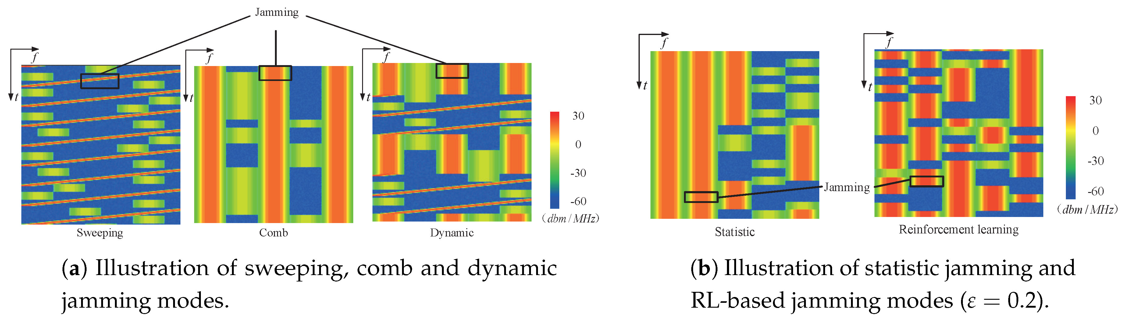
5.1. Simulation Parameters

Consider one transmitter-receiver pair and jammers working in a frequency band of 20 MHz. Both users’ and jammer’s signal were raised cosine waveforms with roll-off factor $\eta =0.6$ and performed full-band detection every $t_s=1$ ms with $\Delta f=100$ kHz. The bandwidth of the jammer and transmitter was 4 MHz. So, the number of actions set $∥{\mathcal{A}}_j∥=5$. The jamming power was 30 dBm. The signal power was 0 dBm. Demodulation threshold ${\beta }_{th}$ was 10 dB. Five kinds of jamming modes were considered against DRL-based user:

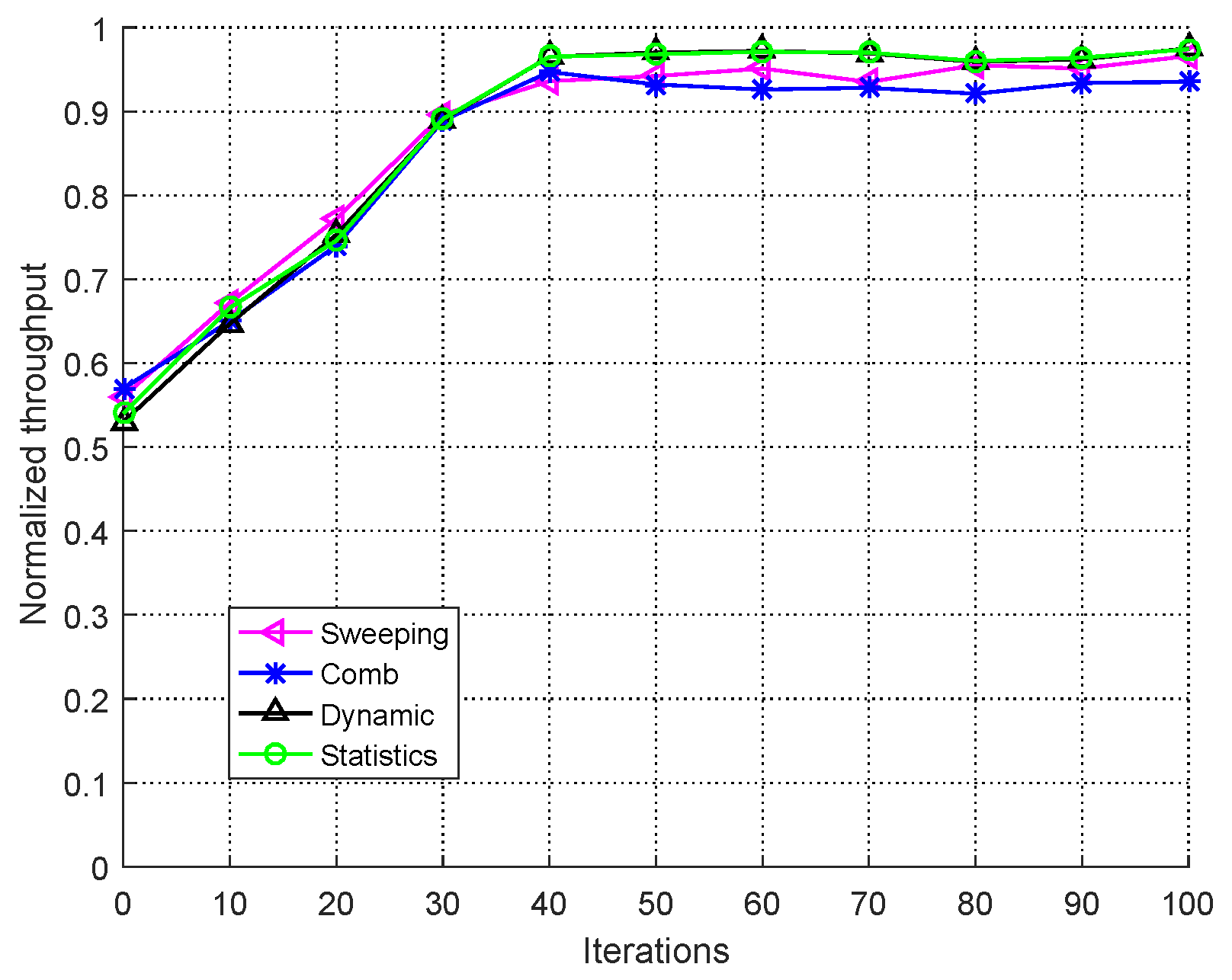
• Sweeping jamming (sweeping speed is 0.8 GHz/s);
• Comb jamming (jamming at 2 MHz, 10 MHz, and 18 MHz simultaneously);
• Dynamic jamming (change the sweeping and comb jamming patterns periodically for every 100 ms);
• Jamming based on statistics (select top three the most frequently used channels by users in 100 ms);
• RL-based jamming method (jamming three bands).

Figure 4a shows the spectrum waterfall of the first three jamming modes where the horizontal axis represents frequency and the longitudinal axis represents time. The simulation results of them combating with a DRL-based anti-jamming method can be seen in [24]. The patterns of jamming based on statistics and RL were dynamically changing according to user’s signal, which can be seen in Figure 4b.

Three kinds of users are taken into consideration against the RL-based jammer:

• Frequency-fixed user;
• Frequency-hopping user with frequency hopping table shown in

  Table 1. Frequency hopping table.

  Current frequency	2 Mhz	6 Mhz	10 Mhz	14 Mhz	18 Mhz
  Next hop	18 Mhz	14 Mhz	2 Mhz	10 Mhz	6 Mhz

  ;
• DRL-based user [24].

According to paper [40], the floating-point operations per second (FLOPS) of DRL in our simulation test was ${10}^9$, and processing speed magnitude of normal CPU was ${10}^{11}$ FLOPS. By now, the embedded neural-network processing unit (NPU) can reach $1.6\times {10}^{13}$ FLOPS. It is likely to run DRL algorithm in many scenarios, such as [41,42], underwater, unmanned aerial vehicle (UAV) systems in future.

5.2. Performance Analysis of User versus Jammers

In order to investigate the performance of DRL-based anti-jamming algorithm and verify the theoretical analysis in Section 4, we let the DRL-based users combat different kind of jammers. In Figure 5, the horizontal axis represents cumulative iterations. Each iteration indicates 2 s (200 times) of the users’ communication. The longitudinal axis is the normalized throughput in one iteration. In Figure 5, four kinds of jammer jam DRL-based user. It can be seen that in the face of four types of jamming, DRL-based user can almost perfectly avoid the jamming signal after training.

In order to illustrate the effect of randomness on the DRL-based anti-jamming algorithm, Figure 6 shows the throughput against RL-based jammer with different $\epsilon$. As we can see in Figure 6, if the RL used a greedy strategy ($\epsilon =0$) completely, after 50 iterations the jammer failed. As $\epsilon$ increased, the performance of DRL anti-jamming dropped dramatically. The deep neural network did not converge due to the randomness, which caused the failure of DRL-based user to learn the pattern of RL-based jamming. From the right of Figure 4b we can see that DRL-based method gets jammed with high probability in face of RL-based jamming.

In Figure 7, the performance of RL-based jammer ($\epsilon =0.2$) combating different modes of users are shown. As we can see, the RL-based jammer can effectively jam the frequency-fixed and frequency-hopping users because the communication process of them are ARP according to the definition in [35]. As expected, since the DRL-based user’s strategy is changing according to the communication effect, the process of user is not ARP, the RL-base jammer can not get its ideal effect because the RL algorithm is not convergent. Note the performance DRL-based mode gets are still unsatisfactory because of $\epsilon =0.2$.

The Figure 8 shows the normalized throughput of different modes of users with different $\epsilon$ after 50 iterations. As we can see, with the $\epsilon$ increasing, the probability to randomly choose actions of RL algorithm increased, which had as a result the jammer overly exploring and the actions with good reward could not be fully exploited. However, as $\epsilon$ increased, the performance of DRL-based user decreased rapidly due to the randomness as explained above.

In

Table 2. Performance comparison of different modes of user and jammer.

	Jammer Mode
	Sweeping		Comb		Dynamic		Statistic		RL ($\mathit{\epsilon }$ = 0.2)
User Mode	Iteration	Normalized Throughput	Iteration	Normalized Throughput	Iteration	Normalized Throughput	Iteration	Normalized Throughput	Iteration	Normalized Throughput
Hopping frequency	\	0.4	\	0.4	\	0.5	\	0.4	10	0.08
Fixed frequency	\	0.4	\	0 or 1	\	0.2 or 0.7	\	0	10	0.08
DRL	50	0.97	50	0.95	50	0.95	50	0.95	∞	0.46

, the performance that different kinds of jammers combat with different kinds of users are summarized. The numbers in the iteration column are the number of iterations that the RL or DRL algorithm needed to converge. The RL-based jamming was used with the setting of $\epsilon =0.2$ in simulation. In the normalized throughput column, the average normalized throughput that is calculated after 50 iterations is shown. As we can see in Table 2, the throughput of DRL-based anti-jamming method was restricted by the RL-based jamming with $\epsilon =0.2$. Due to the good convergent speed and jamming effect of the RL-based jammer, the effective anti-jamming method needs to be further studied.

6. Conclusions

In this paper, we investigated the performance of DRL-based anti-jamming method. We first designed a RL-based jammer. In order to find when the DRL-based method would fail, we first theoretically analyzed the condition when the DRL algorithm couldn’t converge, then we verified the analysis in the simulation part. As the simulation results showed, with the small number of $\epsilon$, the performance of DRL-based user could be effectively restricted by the RL-based jammer with the small $\epsilon$, while RL-based jammer could achieve an excellent jamming effect against common users. In future work, we will study the situations where a user can work on multiple channels simultaneously.

References

1. Pärlin, K.; Alam, M.M.; Le Moullec, Y. Jamming of UAV remote control systems using software defined radio. In Proceedings of the 2018 International Conference on Military Communications and Information Systems (ICMCIS), Warsaw, Poland, 22–23 May 2018; Volume 1, pp. 1–6. [Google Scholar] [CrossRef]
2. Vardhan, S.; Garg, A. Information jamming in Electronic warfare: Operational requirements and techniques. In Proceedings of the 2014 International Conference on Electronics, Communication and Computational Engineering (ICECCE), Hosur, India, 17–18 November 2014; pp. 49–54. [Google Scholar] [CrossRef]
3. Kumar, N.; Kharkwal, N.; Kohli, R.; Choudhary, S. Ethical aspects and future of artificial intelligence. In Proceedings of the 2016 International Conference on Innovation and Challenges in Cyber Security (ICICCS-INBUSH), Noida, India, 3–5 February 2016; pp. 111–114. [Google Scholar] [CrossRef]
4. Zou, Y.; Zhu, J.; Wang, X.; Hanzo, L. A Survey on Wireless Security: Technical Challenges, Recent Advances, and Future Trends. Proc. IEEE 2016, 104, 1727–1765. [Google Scholar] [CrossRef] [Green Version]
5. Liu, X.; Xu, Y.; Cheng, Y.; Li, Y.; Zhao, L.; Zhang, X. A heterogeneous information fusion deep reinforcement learning for intelligent frequency selection of HF communication. China Commun. 2018, 15, 73–84. [Google Scholar] [CrossRef]
6. Jia, L.; Yao, F.; Sun, Y.; Xu, Y.; Feng, S.; Anpalagan, A. A Hierarchical Learning Solution for Anti-Jamming Stackelberg Game With Discrete Power Strategies. IEEE Wirel. Commun. Lett. 2017, 6, 818–821. [Google Scholar] [CrossRef]
7. Jaitly, S.; Malhotra, H.; Bhushan, B. Security vulnerabilities and countermeasures against jamming attacks in Wireless Sensor Networks: A survey. In Proceedings of the International Conference on Computer, Communications and Electronics, Jaipur, India, 1–2 July 2017; pp. 559–564. [Google Scholar]
8. Machuzak, S.; Jayaweera, S.K. Reinforcement learning based anti-jamming with wideband autonomous cognitive radios. In Proceedings of the 2016 IEEE/CIC International Conference on Communications in China (ICCC), Chengdu, China, 27–29 July 2016; pp. 1–5. [Google Scholar] [CrossRef]
9. Mpitziopoulos, A.; Gavalas, D.; Konstantopoulos, C.; Pantziou, G. A survey on jamming attacks and countermeasures in WSNs. IEEE Commun. Surv. Tutor. 2009, 11, 42–56. [Google Scholar] [CrossRef]
10. Du, Y.; Gao, Y.; Liu, J.; Xi, X. Frequency-Space Domain Anti-Jamming Algorithm Assisted with Probability Statistics. In Proceedings of the 2013 International Conference on Information Technology and Applications, Chengdu, China, 16–17 November 2013; pp. 5–8. [Google Scholar] [CrossRef]
11. Jia, L.; Xu, Y.; Sun, Y.; Feng, S.; Yu, L.; Anpalagan, A. A Multi-Domain Anti-Jamming Defense Scheme in Heterogeneous Wireless Networks. IEEE Access 2018, 6, 40177–40188. [Google Scholar] [CrossRef]
12. Liu, Y.; Ning, P.; Dai, H.; Liu, A. Randomized Differential DSSS: Jamming-Resistant Wireless Broadcast Communication. In Proceedings of the 2010 Proceedings IEEE INFOCOM, San Diego, CA, USA, 14–19 March 2010; pp. 1–9. [Google Scholar] [CrossRef]
13. Li, H.; Han, Z. Dogfight in Spectrum: Jamming and Anti-Jamming in Multichannel Cognitive Radio Systems. In Proceedings of the GLOBECOM 2009—2009 IEEE Global Telecommunications Conference, Honolulu, HI, USA, 30 November–4 December 2009; pp. 1–6. [Google Scholar] [CrossRef]
14. Yao, F.; Jia, L.; Sun, Y.; Xu, Y.; Feng, S.; Zhu, Y. A hierarchical learning approach to anti-jamming channel selection strategies. Wirel. Netw. 2019, 25, 201–213. [Google Scholar] [CrossRef]
15. Yu, L.; Li, Y.; Pan, C.; Jia, L. Anti-jamming power control game for data packets transmission. In Proceedings of the 2017 IEEE 17th International Conference on Communication Technology (ICCT), Chengdu, China, 27–30 October 2017; pp. 1255–1259. [Google Scholar] [CrossRef]
16. Popper, C.; Strasser, M.; Capkun, S. Anti-jamming broadcast communication using uncoordinated spread spectrum techniques. IEEE J. Sel. Areas Commun. 2010, 28, 703–715. [Google Scholar] [CrossRef]
17. Hamza, T.; Kaddoum, G.; Meddeb, A.; Matar, G. A survey on intelligent MAC layer jamming attacks and countermeasures in WSNs. In Proceedings of the 2016 IEEE 84th Vehicular Technology Conference (VTC-Fall), Montreal, QC, Canada, 18–21 September 2016; pp. 1–5. [Google Scholar]
18. Jameel, F.; Wyne, S.; Kaddoum, G.; Duong, T.Q. A comprehensive survey on cooperative relaying and jamming strategies for physical layer security. IEEE Commun. Surv. Tutor. 2018. [Google Scholar] [CrossRef]
19. Bayram, S.; Vanli, N.D.; Dulek, B.; Sezer, I.; Gezici, S. Optimum Power Allocation for Average Power Constrained Jammers in the Presence of Non-Gaussian Noise. IEEE Commun. Lett. 2012, 16, 1153–1156. [Google Scholar] [CrossRef] [Green Version]
20. Sagduyu, Y.E.; Berry, R.A.; Ephremides, A. Jamming games in wireless networks with incomplete information. IEEE Commun. Mag. 2011, 49, 112–118. [Google Scholar] [CrossRef]
21. Shamai, S.; Verdu, S. Worst-case power-constrained noise for binary-input channels. IEEE Trans. Inf. Theory 1992, 38, 1494–1511. [Google Scholar] [CrossRef] [Green Version]
22. McEliece, R.; Stark, W. An information theoretic study of communication in the presence of jamming. In Proceedings of the ICC’81: International Conference on Communications, Denver, CO, USA, 14–18 June 1981; Volume 3, pp. 45–3. [Google Scholar]
23. Amuru, S.; Tekin, C.; Van der Schaar, M.; Buehrer, R.M. A systematic learning method for optimal jamming. In Proceedings of the IEEE International Conference on Communications, London, UK, 8–12 June 2015; pp. 2822–2827. [Google Scholar]
24. Liu, X.; Xu, Y.; Jia, L.; Wu, Q.; Anpalagan, A. Anti-Jamming Communications Using Spectrum Waterfall: A Deep Reinforcement Learning Approach. IEEE Commun. Lett. 2018, 22, 998–1001. [Google Scholar] [CrossRef] [Green Version]
25. Henderson, P.; Islam, R.; Bachman, P.; Pineau, J.; Precup, D.; Meger, D. Deep reinforcement learning that matters. arXiv, 2017; arXiv:1709.06560. [Google Scholar]
26. Wang, Q.; Zhan, Z. Reinforcement learning model, algorithms and its application. In Proceedings of the 2011 International Conference on Mechatronic Science, Electric Engineering and Computer (MEC), Jilin, China, 19–22 August 2011; pp. 1143–1146. [Google Scholar] [CrossRef]
27. Xu, Y.; Wang, J.; Wu, Q.; Zheng, J.; Shen, L.; Anpalagan, A. Dynamic Spectrum Access in Time-Varying Environment: Distributed Learning Beyond Expectation Optimization. IEEE Trans. Commun. 2017, 65, 5305–5318. [Google Scholar] [CrossRef] [Green Version]
28. Gwon, Y.; Dastangoo, S.; Fossa, C.; Kung, H.T. Competing Mobile Network Game: Embracing antijamming and jamming strategies with reinforcement learning. In Proceedings of the 2013 IEEE Conference on Communications and Network Security (CNS), National Harbor, MD, USA, 14–16 October 2013; pp. 28–36. [Google Scholar] [CrossRef]
29. Fan, Y.; Xiao, X.; Feng, W. An Anti-Jamming Game in VANET Platoon with Reinforcement Learning. In Proceedings of the 2018 IEEE International Conference on Consumer Electronics-Taiwan (ICCE-TW), Taichung, Taiwan, 19–21 May 2018; pp. 1–2. [Google Scholar] [CrossRef]
30. Singh, S.; Trivedi, A. Anti-jamming in cognitive radio networks using reinforcement learning algorithms. In Proceedings of the 2012 Ninth International Conference on Wireless and Optical Communications Networks (WOCN), Indore, India, 20–22 September 2012; pp. 1–5. [Google Scholar] [CrossRef]
31. Aref, M.A.; Jayaweera, S.K. A novel cognitive anti-jamming stochastic game. In Proceedings of the 2017 Cognitive Communications for Aerospace Applications Workshop (CCAA), Cleveland, OH, USA, 27–28 June 2017; pp. 1–4. [Google Scholar] [CrossRef]
32. Kiumarsi, B.; Vamvoudakis, K.G.; Modares, H.; Lewis, F.L. Optimal and Autonomous Control Using Reinforcement Learning: A Survey. IEEE Trans. Neural Netw. Learn. Syst. 2018, 29, 2042–2062. [Google Scholar] [CrossRef]
33. ZhuanSun, S.; Yang, J.; Liu, H.; Huang, K. A novel jamming strategy-greedy bandit. In Proceedings of the 2017 IEEE 9th International Conference on Communication Software and Networks (ICCSN), Guangzhou, China, 6–8 May 2017; pp. 1142–1146. [Google Scholar] [CrossRef]
34. Amuru, S.; Tekin, C.; van der Schaar, M.; Buehrer, R.M. Jamming Bandits: A Novel Learning Method for Optimal Jamming. IEEE Trans. Wirel. Commun. 2016, 15, 2792–2808. [Google Scholar] [CrossRef]
35. Watkins, C.J.C.H.; Dayan, P. Q-learning. Mach. Learn. 1992, 8, 279–292. [Google Scholar] [CrossRef] [Green Version]
36. Mnih, V.; Kavukcuoglu, K.; Silver, D.; Rusu, A.A.; Veness, J.; Bellemare, M.G.; Graves, A.; Riedmiller, M.; Fidjeland, A.K.; Ostrovski, G. Human-level control through deep reinforcement learning. Nature 2015, 518, 529. [Google Scholar] [CrossRef]
37. Lippmann, R. An introduction to computing with neural nets. IEEE ASSP Mag. 1987, 4, 4–22. [Google Scholar] [CrossRef]
38. Tsitsiklis, J.N.; Roy, B.V. An analysis of temporal-difference learning with function approximation. IEEE Trans. Autom. Control 1997, 42, 674–690. [Google Scholar] [CrossRef] [Green Version]
39. Dayan, P. The convergence of TD (λ) for general λ. Mach. Learn. 1992, 8, 341–362. [Google Scholar] [CrossRef]
40. He, K.; Sun, J. Convolutional neural networks at constrained time cost. In Proceedings of the IEEE conference on computer vision and pattern recognition, Boston, MA, USA, 7–12 June 2015; pp. 5353–5360. [Google Scholar]
41. Xiao, L.; Wan, X.; Su, W.; Tang, Y. Anti-jamming underwater transmission with mobility and learning. IEEE Commun. Lett. 2018, 22, 542–545. [Google Scholar] [CrossRef]
42. Lu, X.; Xiao, L.; Dai, C. Uav-aided 5g communications with deep reinforcement learning against jamming. arXiv, 2018; arXiv:1805.06628. [Google Scholar]
Figure 1. System model.
Applsci 09 01361 g001
Figure 2. Mechanism of reinforcement learning.
Applsci 09 01361 g002
Figure 3. Time-frequency two-dimensional diagram of jammer and user.
Applsci 09 01361 g003
Figure 4. Illustration of jamming modes.
Applsci 09 01361 g004
Figure 5. Performance of deep reinforcement learning (DRL)-based user versus different kind of jammers.
Applsci 09 01361 g005
Figure 6. Performance of DRL-based user versus RL-based jammer with different ε .
Applsci 09 01361 g006
Figure 7. Performance of reinforcement learning (RL)-based jammer with ε = 0 . 2 versus different modes of user.
Applsci 09 01361 g007
Figure 8. Performance of RL-based jammer with different ε versus DRL-based user.
Applsci 09 01361 g008