Abstract
This paper introduces the working principle of the inductive power transfer (IPT) system from the perspective of the electromagnetic field. Using Maxwell’s equations, the analytical solution for the electromagnetic field, synthesized by the primary and secondary circular coils in an IPT system, is deduced in detail to obtain the electric field in the IPT system, and the derivation process is easy to understand for researchers engaged in IPT. The final solutions are obtained by combining analytical derivation and the numerical integration method to find the induced voltage in the secondary coil. Finally, by comparison, the simulation results from the finite element software are in a good agreement with those from the analytical analysis. Moreover, an IPT system is set up to validate the analytical and simulation results, and the maximal relative error is under 6% in different working conditions, which shows that it is feasible to understand the working principle of IPT systems from the viewpoint of the electromagnetic field.
1. Introduction
Inductive power transfer (IPT) technology is a new type of energy transfer method by which energy is transferred from source to load wirelessly, according to the electromagnetic induction theory. In recent years, IPT has developed rapidly and been used for electric vehicles [1,2], biomedical implantable devices [3,4] and wireless charging in intelligent mobile phones [5]. An adaptive four-coil structure was used to improve the power transfer efficiency of the whole system [3]. A square coil was utilized to maximize the power received by the load and the resonant frequency was adjusted to maximize the coil’s quality factor [4]. A mobile phone shell and the coil in the secondary side were used as the resonance bodies, which proposed a novel way to provide electrical energy for a mobile phone [5].
There are many applications for IPT systems, but the power transfer mechanism in between the coupled coils in an IPT system is indistinct. Therefore, research on the mechanism of energy transfer of the coil coupler is very important for IPT technology. Currently, research methods for IPT systems can mainly be classified into two categories: The coupled-mode theory and the equivalent circuit method. These have been proven to be equivalent through analysis with a 4-coil IPT system [6]. In 2007, the team led by Soljačić in MIT (Massachusetts Institute of Technology) elaborated on the analysis and modelling method of the system from the perspective of the coupled-mode theory, which laid a theoretical foundation for the further development and popularization of IPT technology [7]. Coupled-mode theory is used to study the coupling principle of power transmission. The power transfer process from one resonant body to another can be expressed as a first-order partial differential equation according to it. This equation provides an accurate and effective modelling method for IPT systems, as well as an analytical tool to understand the power transfer mechanism in strongly coupled systems. In IPT systems, when the two resonant coils are close, strong coupling exists between them. Under these conditions, with the help of coupled-mode theory, it was found that the energy loss in the primary coil was much slower than the power transferred from the primary coil to the secondary coil [8], thus, the energy transmission was quite efficient. From the perspective of circuit theory and practical applications, the mutual inductance model was used to obtain the relationship between system transfer efficiency and parameters. The mutual inductance model can also be utilized to analyze the power transfer capability as well [9,10].
Although the mutual inductance model is mature, its accuracy depends on the accurate acquisition of the coil parameters. In high-frequency cases, the coil impedance characteristic varies greatly with the operating frequency. Coupled-mode theory has been widely adopted in recent years, but in the analysis process, the state quantities are employed instead of electrical parameters. In addition, the coupled-mode theory model is relatively abstract, and it is difficult to build the mathematical model with lumped circuit parameters. By using the Biot–Savart law, the analytical solution of the electromagnetic field in the IPT system was calculated through the magnetic vector potential. However, the derivation process of the analytical solution of the electric field and magnetic field in IPT systems and the experimental verification were not introduced [11].
In [12], the derivation of the magnetic field, based on the analysis of a current-carrying conductor, is accurately calculated and a good approximation has been done when the far-field is calculated. The mutual inductance and self-inductance of two coaxial coils in a multilayer media have been introduced, and the frequency limitations of magnetic substrates are also established [13]. The far-field solution of a loop of any size is deduced in [14], and the far-field of a square loop is also discussed, finally proving that when the circular and square loops are the same in area and small in size with respect to wavelength, their far-field solutions are identical, but they are different when the size is large in terms of wavelength. From [15], it can be seen that the far-field approximation solution of the electromagnetic field cannot be used in near-field systems because of the large relative percent error. The exact integration of vector potentials of thin circular loop antennas is then introduced to solve this problem.
In this paper, using Maxwell’s equations, the analytical solution for the synthesized electric and magnetic field, both by the primary and secondary circular coil in an IPT system, are deduced in this paper, and the electric field is analyzed in detail. The numerical integration method is used to find the induced voltage in the secondary coil. Finite element software is utilized to compare with the analytical results, and an IPT system is set up to validate the analytical results experimentally.
2. Mutual-Inductance Model of the IPT System
The system structure is given in Figure 1. The alternating current from the source is first converted into a direct current through an AC/DC converter and then into a high-frequency alternating current through another AC/DC converter. Simultaneously, the transmitting coil CoilP converts the electrical energy into electromagnetic energy, and the receiving coil CoilS absorbs the energy from the near-zone electromagnetic field, converting it into electrical energy. The electrical energy is then conveyed through a rectifier to charge the battery. The coupling between the primary and secondary systems is defined as mutual inductance M.
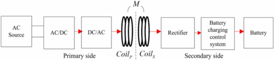
Figure 1.
Inductive power transfer (IPT) system structure.
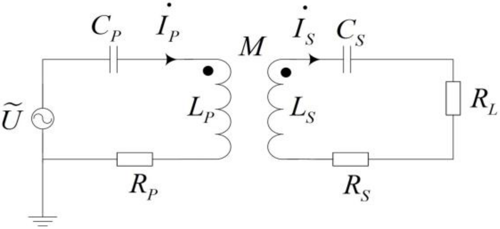
The mutual inductance model is shown in Figure 2. The equivalent series impedances on CoilP and CoilS are RP and RS, respectively. The load impedance is RL. In this paper, the series-series compensation network is used in the IPT system, and compensating capacitors in the primary and secondary side are CP and CS, respectively. The primary side is powered by a voltage source U and the primary circuit current and the secondary circuit current are IP and IS, respectively. According to the KVL equation, the following equations can be obtained:
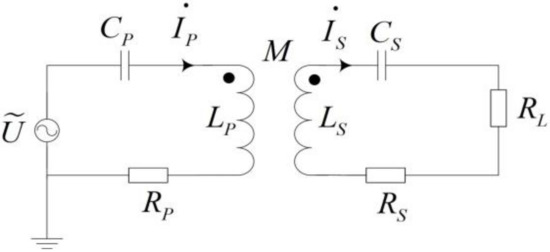
Figure 2.
An IPT system model by mutual inductance.
When the primary and secondary circuits are resonant, . The system efficiency and load power are derived as follows [16]:
Figure 3 shows a schematic of the electromagnetic field around the primary and secondary coil. The sine alternating current in the primary side coil generates the time-harmonic electromagnetic field. We assume that the time-harmonic electric field induced at the position of CoilS is . Then, the integral of on the secondary loop is equal to the induced voltage US. Combined with Figure 2 and Figure 3, the following expression is obtained:
where dlS is a directional micro-element on the secondary side coil. In this paper, the bold symbols represent space vectors.
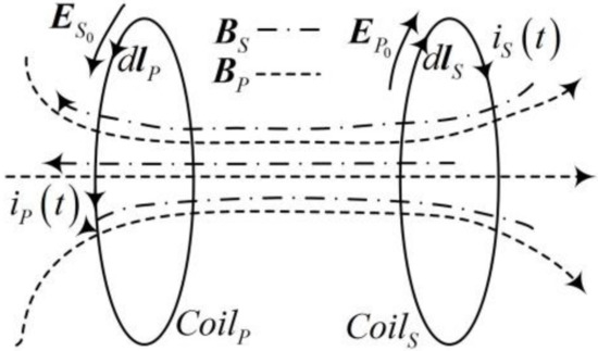
Figure 3.
Schematic of field distribution around the primary and secondary coil.
Similarly, the corresponding time-harmonic electric field will be generated around CoilP by the induced current in the secondary coil. The corresponding induced voltage is . Therefore, the working principles of an IPT system can be understood from the perspective of an electromagnetic field. In Section 3, Maxwell’s equations are used to calculate the electric fields generated by the primary and secondary coil in detail, and the derivation process is easy to understand for researchers engaged in IPT.
3. Analytical Solution of the Time-Harmonic Electromagnetic Field around One Current-Carrying Coil
In this section, the electromagnetic field generated by the primary and secondary coil in an IPT system is deduced in detail by Maxwell’s equations.
3.1. Maxwell’s Equations in the Complex Domain
Maxwell’s equations in the complex domain can be written as follows:
where H, B, E, D, J, JS, ρ and are the magnetic field strength, magnetic flux density, electric field, electric displacement field, polarization current density, free current density in space and free electric charge density, respectively.
The following relationships exist in an isotropic linear medium:
where ɛ, μ and σ are the permittivity, permeability and conductivity of the medium, respectively. By comparison of Equations (6) and (7), it can be found that the forms of Maxwell’s equations in the complex domain are simpler.
3.2. Current Density of a Current-Carrying Coil
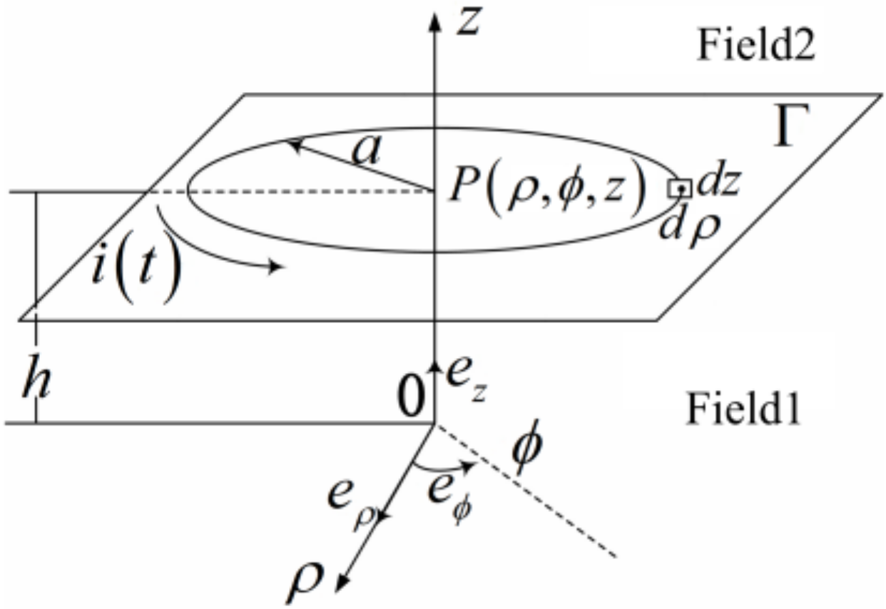
Due to the circular structures of the primary and secondary coils in the IPT system, a cylindrical coordinate was adopted to analyze the system. The three directions of the cylindrical coordinate system are denoted as eρ, eϕ and ez, as shown in Figure 4. The radius of the coil is a and the height is h. Fields 1 and 2 are the regions above and below plane Г, respectively.

Figure 4.
Schematic of a coil.
Because the direction of the free current density is the same as eϕ and current only exists in the coil, the current density at any point P(ρ,ϕ,z) can be expressed as follows:
where C2 is an undetermined coefficient affected by the external current.
Therefore, with a directional micro-section dS = dρdzeϕ as shown in Figure 4, the integral form of current I of the coil is shown as follows:
where S is a hypothetical surface through which the current density of a circular coil passes vertically.
Thus, the current density of the coil is JS = Iδ(ρ − a)δ(z − h)eϕ. When the number of coil turns are N, ignoring the radius of the wire, the current flowing through the directional micro-section dS is NI, and the current density at the corresponding location is JS(P) = NIδ(ρ − a)δ(z − h)eϕ.
3.3. Analytical Solution of the Electric Field
The following relationships exist in the cylindrical coordinate system:
where P represents a space vector and Ψ is a scalar value.
By combining Equations (6), (10)–(12), and by rearranging Equation (7), then
where k2 = −jωμ(σ + jωε).
Meanwhile, JS·eρ = JSρ = JS·ez = JSz = 0 and ∂JSϕ/∂ϕ = 0, so the divergence of the current density is
Therefore, Equation (19) can be written as
If there is no free current density, then Equation (19) can be expressed as
Replacing the space vector P by Ei in Equation (15) yields
where i = 1 and 2, representing fields 1 and 2.
By defining A = , B = , C = , and D = , substituting Equation (23) into Equation (17), the gradient of the divergence of Ei can be expressed as A + B + C + D, where
Replacing the space vector P by Ei in (16) yields
Similarly, can be calculated by applying Equation (16) again.
In cylindrical coordinates,eρ·eϕ = 0, eρ·ez = 0 and eρ·eρ = 0. Thus,
Rearranging Equations (24)–(27) yields
The relationship exists in any orthogonal coordinate system, so in the cylindrical coordinate system,
Taking the dot product between both sides of Equation (31) and applying Equations (29) and (30), the following relationship can be obtained:
According to the symmetry, it is easily derived that the electric field only exists in the ϕ direction, and its intensity is angle independent, which means that E = Eϕ·eϕ and . Thus,
Similarly,
According to Equation (34), Equation (22) can be written as
Defining Eiϕ = R(ρ)Z(z) and using the method of separation of variables in Equation (36) yields
By defining the first and second parts of the left side of Equation (37) as H(ρ) and Z(z), respectively, it can be easily found that H(ρ) and Z(z) are linearly independent. Thus,
where λ is a separation variable [17].
R(ρ) can be calculated because the time-harmonic electromagnetic field is bounded and non-zero:
where J1 is a Bessel function of the first kind.
With the formulas of R(ρ) and Z(z), the expression of Eiϕ can be finally obtained as follows:
Because Eiϕ is zero at infinity, and E2ϕ − E1ϕ = 0 and are satisfied on the plane Г, then:
where
4. Electric and Magnetic Field in the IPT System
In this section, the analytical solutions for the electric and magnetic field, induced both by the primary and secondary coil, are deduced, and the numerical integration method is used to acquire numerical results.
4.1. Analytical Solution of the Electric and Magnetic Field
As shown in Equation (7), there is a one-to-one correspondence between the electric field E and the magnetic flux density B. When the analytical solution of E is obtained, the analytical solution of B can also be uniquely determined. Thus, in this section, the electric field is calculated only.
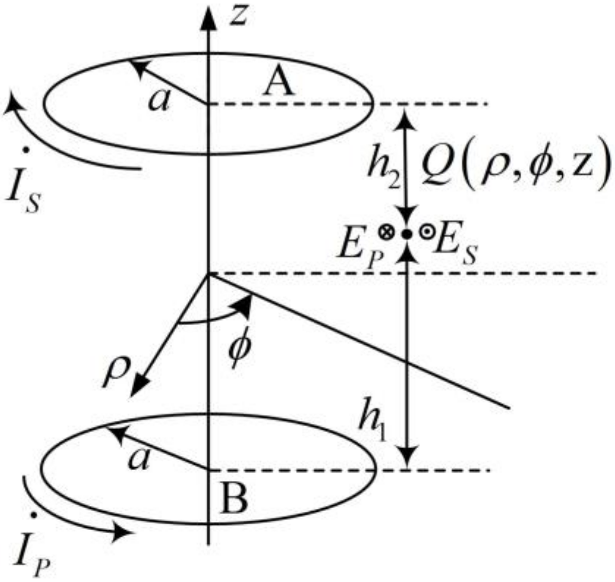
An electric field illustration of the sampling point in the double-coil system is given in Figure 5. The radius of each coil is a. The current in the primary and secondary coil is defined as IP and IS, respectively. NP and NS are the numbers of turns in the two coils, respectively. The distances from CoilP and CoilS to the point Q are denoted as h2 and h1, respectively.
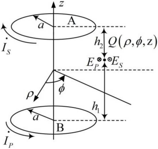
Figure 5.
Illustration of the electric field at a sampling point of the double-coil IPT system.
The electric field only exists along the ϕ direction. Thus, by combining Equations (2) and (5), when the system is operated at its resonant frequency, the following equation can be obtained:
where is the electric field at CoilS produced by the current in CoilP:
The total electric field at point Q is E = EP + ES, and
where EP and ES are the electric fields produced by the current in the primary and secondary coils, respectively. Equations (46) and (47) laid the base for the next step numerical calculations to find the distribution of the E and H field.
4.2. Numerical Integration Method for the Analytical Solution
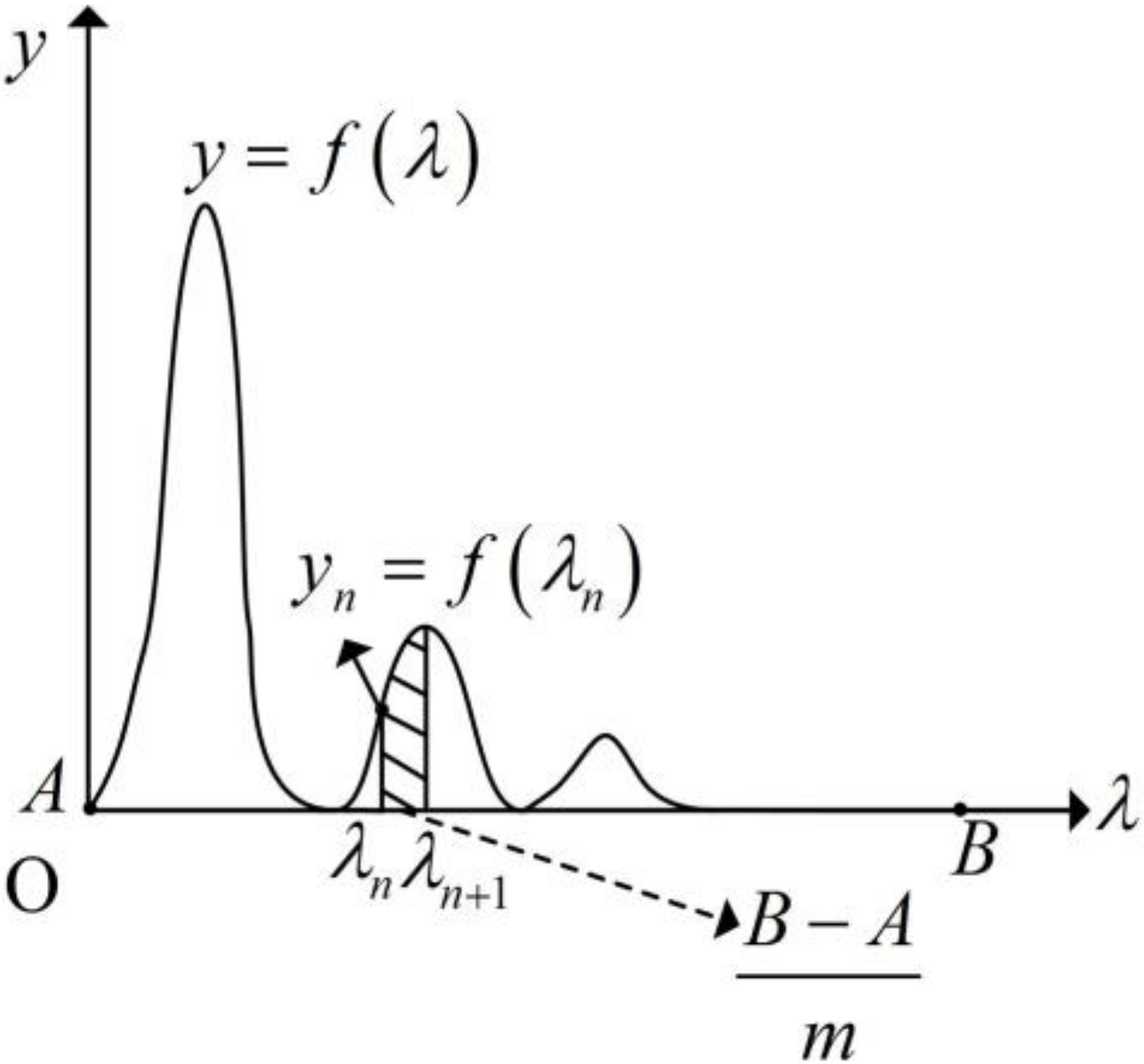
The integral of the function in Equation (46) needs to be calculated and the integration interval is from A to B.
Since it is difficult to determine the primitive function of the integrand f(λ), the integration method is used to acquire an approximation result. In the numerical integration method, the integration interval is divided into parts, and the sum of their areas is the approximation of the integral of the function f(λ) from A to B.

Figure 6.
Numerical integration method for the analytical solution.
If m tends to infinity, then
In Equation (46), A is equal to zero. When a = ρ = 0.1 and λ = 1000, f(λ) tends to zero, so the upper limit of the integral, (i.e., B) can be set to be 1000. To ensure accuracy, the number of tiny intervals was defined as m = 1 × 10⁵.
The final solutions are obtained by combined analytical derivation and numerical calculations. In the next section, the analytical solution is verified by simulation.
5. Simulation Verification
In this section, MATLAB is used to provide the numerical results of analytical solutions and the simulation results are obtained through use of the finite element software COMSOL. The analytical solution is coincident with the simulation results, which shows the accuracy of analytical solution deduced in Section 3.
5.1. Simulation Verification of the Electric Field Produced by a Single-Turn Current-Carrying Coil
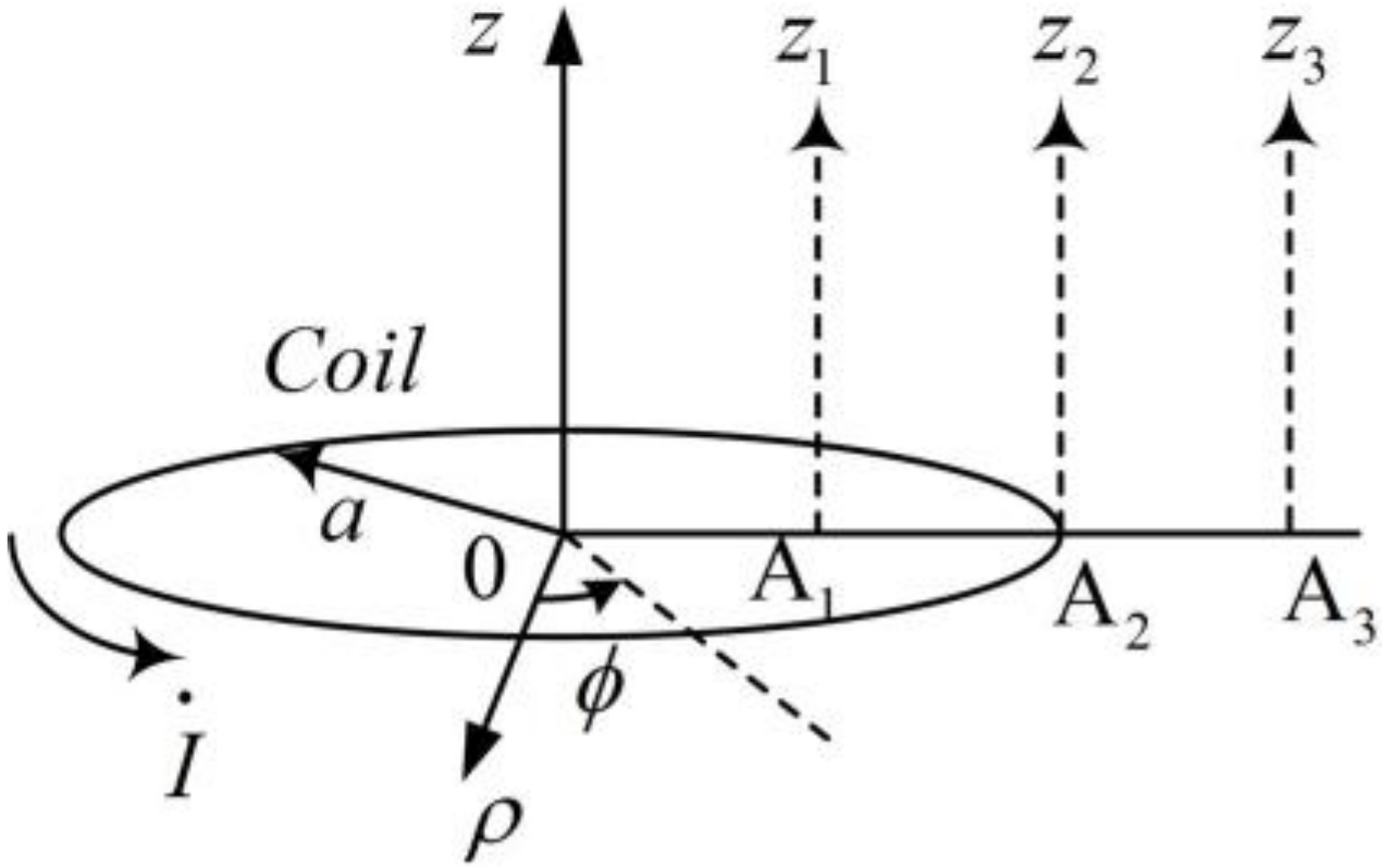
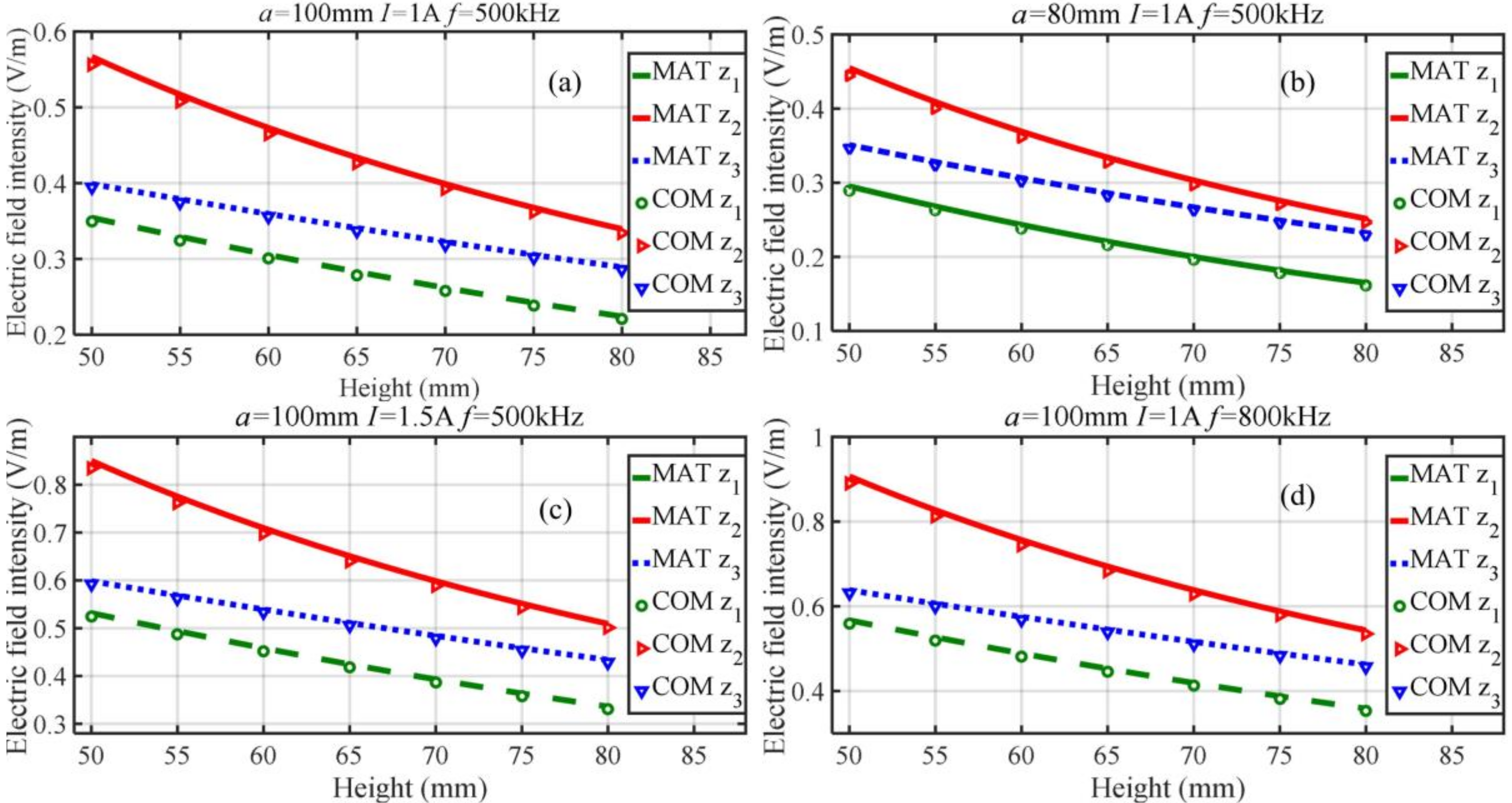
As shown in Figure 7, the radius of the coil is a and the coordinates of points A1, A2 and A3 are (a/2, π/2, 0), (a, π/2, 0) and (3a/2, π/2, 0), respectively. The moduli of the electric field, changing with z at z1, z2 and z3, are given in Figure 8a–d, where I and f denote the effective current value and the frequency in the coil, respectively. In Figure 8, MAT represents the results obtained by the analytical results of electric field using MATLAB, and COM represents the simulation results using the finite element software COMSOL.
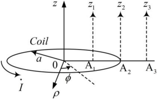
Figure 7.
The three points are in ρ axis.
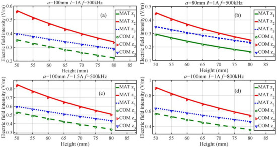
Figure 8.
Electric-field intensity at different positions. (a) is the electric field curve when a = 100 mm, I = 1 A and f = 500 kHz, (b) is the electric field curve when a = 80 mm, I = 1 A and f = 500 kHz, (c) is the electric field curve when a = 100 mm, I = 1.5 A and f = 500 kHz, (d) is the electric field curve when a = 100 mm, I = 1 A and f = 800 kHz.
The analysis results coincide with the simulation results and the maximal relative error is below 1%. This is because the analytical solution was deduced under the assumption that the current-carrying coil is treated as a wire with no cross section. Since the distance from the test point to the current-carrying coil is much longer than the coil diameter, the relative error caused by the coil diameter can be ignored. Similarly, the accuracy of the analytical solution of the magnetic field strength can be verified also.
5.2. Simulation Verification of the Electric Field in the IPT System
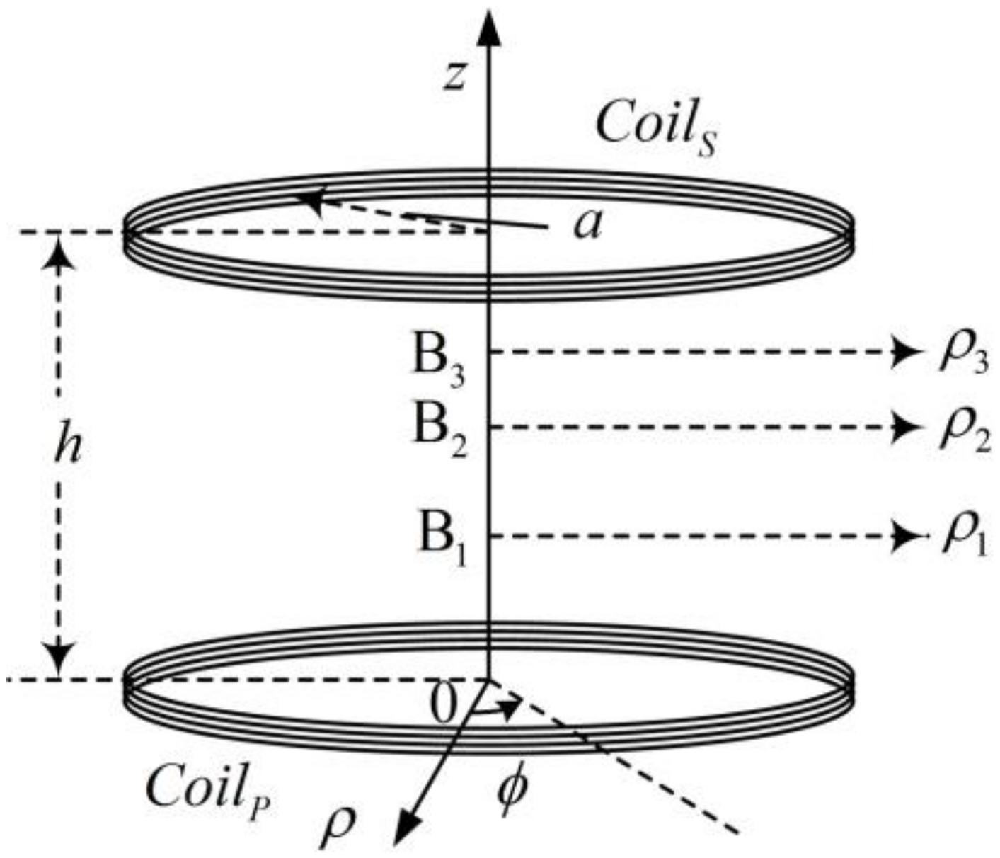
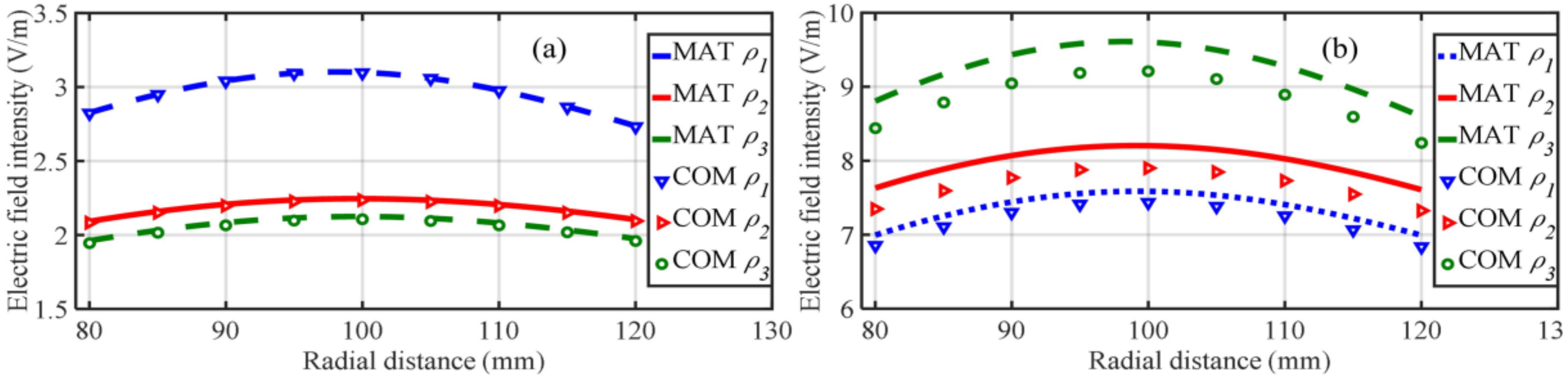
As shown in Figure 9, the radii of the two coils are both a = 100 mm, the distance between them is h = 100 mm, and they both have N turns. The coordinates of points B1, B2 and B3 are (0, 0, h/3), (0, 0, 5h/9), and (0, 0, 2h/3), respectively. The circuit topology is shown in Figure 2, and in the circuit, RL = 5 Ω and the system resonant frequency is f0 = 500 kHz when the effective value of the current IP in the primary coil is 1 A. The obtained moduli of the electric field, changing with ρ at ρ1, ρ2 and ρ3, are given in Figure 10a,b.

Figure 9.
The three points are located in the z-axis.
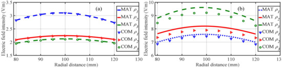
Figure 10.
Analytical and simulated synthesized electric-field intensity with different N values. (a) is the electric field curve when the number of coil turns on both sides is 4, (b) is the electric field curve when the number of coil turns on both sides is 8.
The symbols MAT and COM have the same meanings as those in Figure 8. The maximum deviation between the results obtained with these two methods is 4.3% under the condition that the number of turns of both coils is 8 and that the test point on ρ3 is the closest point to the secondary coil. When the number of coils turns increases, the total height of the coil becomes larger compared with the results when N = 4, and the current distribution in the coil becomes much more complex, where the relative error turns out to be larger when the test point is nearer to the coil. However, it is still an acceptable relative error. Hence, Figure 10 verifies that the formula E = EP + ES can be used for the calculation of total electric field between coupled coils in an IPT system. Similarly, for the magnetic field strength, H = HP + HS can also be verified. In the next section, an IPT experimental system is set up to further validate the analytical solution.
6. Experimental Verification
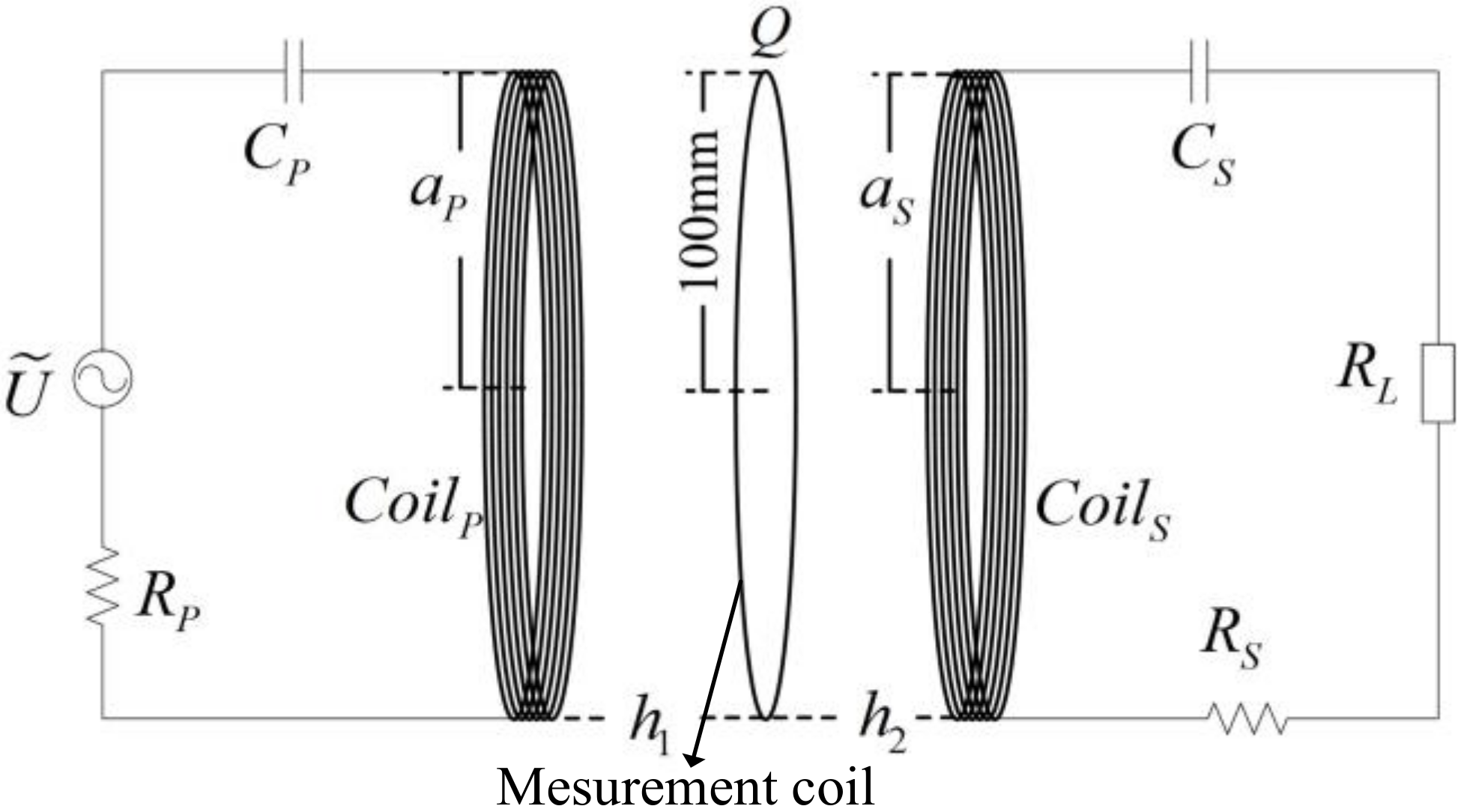
The electric field intensity cannot be measured directly. According to Equation (42), the electric field generated by the coil is along the ϕ direction, but the electric field intensity is independent of ϕ. For a single-turn measurement coil, when its plane is oriented parallel to the plane of the current-carrying coil, the electric field intensity can be measured using the relationship U = ∮l|E|dl. When current flows in the source coil and the measurement coil is opened, the relationship between the open-circuit voltage and the circular electric-field strength at the measurement coil can be expressed as |E| = U/(2πa), in which a is the radius of the measurement coil. The experimental configuration is shown in Figure 11.

Figure 11.
Experimental configuration.
By changing the position and size of the measurement coil, the variation of the electric-field strength at different positions can be measured, where Q is an arbitrary point on the measurement coil. To facilitate the experiment, the radius of the measurement coil was set equal to the radius of the primary and secondary coils.
When the secondary side is at resonant state, the reflected impedance from the secondary side to the primary side is purely resistive, while the resonant frequency of the primary side is independent of the secondary side. The experimental steps were as follows [18]:
Firstly, a compensation capacitor with CS = 1000 pF, a load with RL = 20 Ω and an adjustable current source were connected in series with the primary coil. The current source frequency was adjusted to a specific value so that the load current and voltage were in the same phase, which is the resonant frequency. In the experiment, the measured resonant frequency was set at f0 = 486.7 kHz. Then, the current source was removed and the secondary side of the circuit was connected as shown in Figure 11.
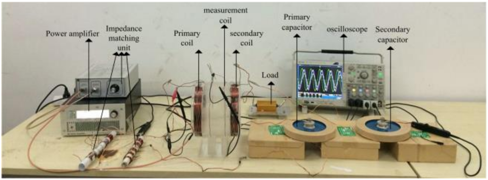
Secondly, to achieve full resonance (i.e., the primary side and secondary side are both resonant), a compensation capacitor must be connected in series with the primary coil. The experimental circuit configuration is shown in Figure 11. The experimental set up is shown in Figure 12, and the frequency of the power amplifier shown in Figure 12 was maintained at f0 = 486.7 kHz, and the compensation capacitance CP was adjusted until the voltage and current of the power source were in the same phase, at which point the circuit achieves full resonance.

Figure 12.
Experimental set-up.
The relevant parameters are listed in Table 1.

Table 1.
Experimental parameters.
Finally, different values of h1 in Figure 11 were chosen, and the output current of the power amplifier was changed. The corresponding induced voltages of the measurement coil at different positions were measured. The voltage was divided by the perimeter of the measurement coil to obtain the electric field intensity at that point.
Figure 13 shows waveforms of the experiment result, measured by Tektromix DPO4104B when the effective current on the primary side was 0.499 A and h1 = 52 mm. The purple line is the primary side current ip, the dark blue line is the output voltage of the power amplifier up, the green line is the induced current in the secondary side coil is and the light blue line is the induced voltage of the measurement coil um.
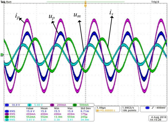
Figure 13.
Waveforms of primary voltage up, primary current ip, secondary current is and induced voltage um of the measurement coil.
The experimental results of electric field intensity at different h values are shown in Figure 14. H1, H2 and H3 represent values of h1 at 27 mm, 52 mm and 80 mm, respectively. The largest relative error, which is below 6%, happens under the experimental condition that h1 = 80 mm, and the maximal relative error is below 2% at the other two positions. The reason why the analytical solution is always larger than the experiment data is that during the numerical integration, the coil resistance is not considered. It can be found that near the primary side, the analytical solution is just a little higher than the experiment data, the reason for this is that near the primary side the electric field intensity is determined dominatingly by the current in primary side. It is reasonable to believe that the experiment has validated the analytical solution.
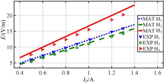
Figure 14.
Electric field intensity at different h1 values.
7. Conclusions
To reveal the energy transfer mechanism in the IPT system, it is important to study the distribution of the time-harmonic electric and magnetic fields in the IPT system. In this paper, the analytical solution of the time-harmonic electric and magnetic fields in an IPT system was deduced in detail, and the numerical integration method was used to find the distribution of the E and H fields on the basis of the analytical solution.
Firstly, based on the Maxwell’s equations, the Laplacian of the electric field and the magnetic field strength around the current-carrying coil were derived theoretically. The analytical expression of the electric field was calculated in an integral form, and the result can be obtained by the simple trapezoidal integration method. The final solutions were obtained by combined analytical derivation and numerical calculations.
Secondly, the correctness of the analytical results for the electromagnetic field in the IPT system was verified utilizing the finite element software COMSOL.
Finally, an IPT system was set up, and the electric-field strength between the primary and secondary coils was measured. The experimental results further verify the correctness of the analytical solution. The analytical solution developed in this paper can be applied to analyze electric and magnetic fields in any uniform medium.
Author Contributions
K.Z. proposed the idea, obtained the results and wrote the paper. K.Z. and X.R. built the experiment setup. All authors together contributed by drafting and critical revisions.
Funding
This work was supported by the Seed Foundation of Innovation and Creation for Graduate Students in Northwestern Polytechnical University.
Conflicts of Interest
The authors declare no conflict of interest.
References
- Siqi, L.; Mi, C. Wireless Power Transfer for Electric Vehicle Applications. IEEE J. Emerg. Sel. Top. Power Electron. 2015, 3, 4–17. [Google Scholar] [CrossRef]
- Shin, J.; Shin, S.; Kim, Y.; Ahn, S.; Lee, S. Design and Implementation of Shaped Magnetic-Resonance-Based Wireless Power Transfer System for Roadway-Powered Moving Electric Vehicles. IEEE Trans. Ind. Electron. 2014, 61, 1179–1192. [Google Scholar] [CrossRef]
- Kyungmin, N.; Heedon, J.; Sai, K.O.; Franklin, B. An improved wireless power transfer system with adaptive technique for Implantable Biomedical Devices. In Proceedings of the 2013 IEEE MTT-S International Microwave Workshop Series on RF and Wireless Technologies for Biomedical and Healthcare Applications (IMWS-BIO), Singapore, 9–11 December 2013. [Google Scholar]
- Guilin, S.; Badar, M.; Ying, L.; Qi, Z. Ultracompact Implantable Design with Integrated Wireless Power Transfer and RF Transmission Capabilities. IEEE Trans. Biomed. Circuits Syst. 2018, 12, 281–291. [Google Scholar]
- Nathan, S.J.; Francesco, C. Enabling wireless power transfer though a metal encased handheld device. In Proceedings of the 2016 IEEE Wireless Power Transfer Conference (IPTC), Aveiro, Portugal, 5–6 May 2016. [Google Scholar]
- Shou, W.; Dawei, G. Power transfer efficiency analysis of the 4-coil wireless power transfer system based on circuit theory and coupled-mode theory. In Proceedings of the 2016 IEEE 11th Conference on Industrial Electronics and Applications (ICIEA), Hefei, China, 5–7 June 2016; pp. 1230–1234. [Google Scholar]
- Rafif, E.H.; Aristeidis, K.; Joannopoulos, J.D.; Marin, S. Efficient weakly-radiative wireless energy transfer: An EIT-like approach. Ann. Phys. (N. Y). 2009, 324, 1783–1795. [Google Scholar]
- Manasi, B.; Vikaram, S.; Chirag, W. Transmission of Wireless Power in two-coil and four-coil systems using coupled mode theory. In Proceedings of the 2015 IEEE Aerospace Conference, Big Sky, MT, USA, 7–14 March 2015. [Google Scholar]
- Mihai, D.R.; Robin, T.; Rard, A.; Tan, Y.K.; Jan, K.S. Numerical and experimental study of the effects of load and distance variation on wireless power transfer systems using magnetically coupled resonators. In Proceedings of the 9th IET International Conference on Computation in Electromagnetics (CEM 2014), London, UK, 31 March–1 April 2014. [Google Scholar]
- Hiroshi, H.; Yuki, O.; Nobuyoshi, K.; Kunio, S. Equivalent circuit of induction fed magnetic resonant IPT system. In Proceedings of the 2011 IEEE MTT-S International Microwave Workshop Series on Innovative Wireless Power Transmission: Technologies, Systems, and Applications, Kyoto, Japan, 12–13 May 2011; pp. 239–242. [Google Scholar]
- Song, X.; Liu, G.; Li, Y.; Zhang, C.; Xu, X. Analyses and experiments of field-circuit coupling equations for wireless power transfer using solenoidal coils. In Proceedings of the 2015 IEEE International Wireless Symposium (IWS 2015), Shenzhen, China, 30 March–1 April 2015. [Google Scholar]
- Scholz, P. Analysis and Numerical Modeling of Inductively Coupled Antenna Systems. Ph.D. Thesis, Technique University Darmstadt, Darmstadt, Germany, 2010. [Google Scholar]
- Hurley, G.H.; Duffy, M.C. Calculation of self- and mutual impedances in planar sandwich inductors. IEEE Trans. Magn. 1997, 33, 2282–2290. [Google Scholar] [CrossRef]
- Kraus, J.D. The Loop Antenna. In Antennas, 2nd ed.; McGRAW-Hill International Publishing Company: New York, NY, USA, 1988; Chapter 6. [Google Scholar]
- Douglas, H.W. An exact integration procedure for vector potentials of thin circular loop antennas. IEEE Trans. Antennas Propag. 1996, 44, 157–165. [Google Scholar]
- Marinus, P.; Friedrich, W.F. Development of a 5 kW Inductive Power Transfer System Including Control Strategy for Electric Vehicles. In Proceedings of the International Exhibition and Conference for Power Electronics, Intelligent Motion, Renewable Energy and Energy Management, Nuremberg, Germany, 20–22 May 2014. [Google Scholar]
- Frank, O. Boundary integral equation technique defined on a spherical surface with different applications in electromagnetics and acoustics. In Proceedings of the IEEE Antennas and Propagation Society International Symposium and URSI National Radio Science Meeting, Seattle, WA, USA, 20–24 June 1994. [Google Scholar]
- Yabiao, G.; Zion, T.H.T.; Antonio, G. Analytical method for mutual inductance and optimum frequency calculation in a series-series compensated inductive power transfer system. In Proceedings of the 2017 IEEE Applied Power Electronics Conference and Exposition (APEC), Tampa, FL, USA, 26–30 March 2017. [Google Scholar]


© 2019 by the authors. Licensee MDPI, Basel, Switzerland. This article is an open access article distributed under the terms and conditions of the Creative Commons Attribution (CC BY) license (http://creativecommons.org/licenses/by/4.0/).