Abstract
To test the nonlinearity and non-stationarity of measured dynamic signals from a bridge structure with high-level noise and dense modal characteristics, a method that combines the adaptive signal decomposition with the recurrence analysis is proposed to solve the difficulty of testing nonlinearity and non-stationarity of bridge structure signals. A novel white noise assistance and cluster analysis are introduced to the ensemble empirical mode decomposition to alleviate mode-mixing issues and generate single-mode intrinsic mode functions. Combining the hypothesis-testing scheme of nonstationary and nonlinear synchronization and surrogate techniques, a data-driven recurrence quantification analysis method is proposed and a novel recurrence quantification measure pairs are set up. To demonstrate the efficacy of the proposed methodology, complex signals, which are collected from a carefully instrumented model of a cable-stayed bridge, are utilized as the basis for comparing with traditional nonlinear and non-stationary test methods. Results show that the proposed multiscale recurrence method is feasible and effective for applications to a nonlinear and non-stationary test for real complex civil structures.
1. Introduction
With the fast advancement of microprocessors, miniature sensors, wired and wireless digital transmission networks, and contemporary monitoring devices are able to collect an enormous amount of signals exhibited from bridge structures. However, it is well known that complex bridge structures show high-level nonlinear and non-stationary behaviors due to a variety of causes such as continuous ambient vibrations, vehicle-bridge coupling effect, cumulative crack growth, and degradation of columns, joints, and beams [1]. This brings considerable challenges for civil engineers to inspect the time-varying performance of complex bridge structures. It is of great significance to consider the characteristics of bridge structure signals for detecting the inherent non-stationary and nonlinear nature of signals.
Conventional stationary analysis methodologies and linear statistical approaches tend to have limitations to capture the nonlinear and nonstationary variations in the signals [2]. For example, the fast Fourier transformation cannot provide the temporal localization of the frequency components and assumes that spectral components are stationary. Furthermore, linear statistical methods, e.g., regression models or the analysis of variance, have certain difficulties to capture the nonlinearity and non-stationarity of signals. As a result, linear and stationary methods lead to less realistic characterization and estimation of time series from real-world bridge structures.
In recent decades, the recurrence plot (RP) and the recurrence quantification analysis (RQA) has already become a commonly powerful tool for its better understanding and interpretation of complex dynamic behaviors [3]. RP is usually utilized to give a qualitative visual impression of the dynamics of a given system. It is essentially a global probabilistic autocorrelation function that consider the relative frequencies at which a system returns to a given dynamic state [4]. Based on the recurrence point density, the diagonal and vertical line distribution in RP [4], RQA [5] is proposed to quantify the structures displayed by RP. Compared with many classical signal-processing methods, e.g., Fourier transform-based methods, RP and RQA have the distinct advantage of sensitivity to some varying dynamic properties and is relatively immune to noise [5].
In recent years, RP and RQA or their variations, like cross recurrence plot [6], the ordinal patterns recurrence plot [7], the multivariate recurrence plot [8], and the recurrence network [9] have been widely and successfully applied to test the nonlinearity and non-stationarity of the signal from the real world in various branches of science and technology, such as in physiology [9,10,11,12], economy [13,14], chemistry [15,16], and engineering [17,18]. Marwan et al. [1] and Zbilut et al. [19] presented excellent reviews of the earlier studies on RP and RQA. In addition, recent reviews by Catone et al. and Webber et al., covering detailed and extensive theories and various application, are available in References [6,20].
Although powerful in testing the properties of nonlinear and nonstationary signals, the success of RP and RQA application is mainly on the signal from the numerical simulation or small-scale and controlled laboratory experiments [6,20]. In these research studies, the influencing factors of the experiments are controllable and RP patterns of the signals are simple. However, when being used in the measured signals from bridge structures, RP and RQA faces several requirements of the bridge dynamic signal processing [21]: (1) high-level noise, (2) multi-mode and closely spaced mode, and (3) data-driven. On one hand, as summarized above, RP and RQA are usually effective when dealing with the signal with a single recurrence mode and low-level noise. However, bridge structures are generally large and complex systems. The signals from bridge structures are influenced by intrinsic and extrinsic factors (e.g., the rich structural information, the existence of high-level noise effect), which lead to inaccurate and spurious results by using RP and RQA. On the other hand, the choice of parameters of RP, especially the crucial recurrence threshold, mainly depends on the goal of the analysis [22,23], which seriously restrict the application of RP and RQA in civil engineering.
Recently, Xiong et al. [24] and Gao et al. [25] made some worthy contributions in this area where the complex traffic flow signals had been dealt with by using a combination of empirical mode decomposition (EMD) and the RP method. The multiscale framework has been considered a promising solution to explore recurrence dynamics in complex systems [1]. However, an undesirable disadvantage of EMD is the mode mixing effect when applied in the field of signal processing [21,26]. This means that oscillations or frequencies with the same time scale are assigned to different decomposed modes or the oscillations of disparate amplitudes that appear in one mode [27]. In order to lessen this problem, the ensemble EMD (EEMD) [28] has been proposed as an adaptive noise-assisted method capable of providing a partial solution to the mode-mixing problem. However, this method may produce spurious frequencies due to the added white noise and has difficulties estimating closely spaced frequencies [27].
In this regard, two new works have been done in this paper. First, an improved EEMD method is developed to alleviate the mode-mixing problem of EEMD in order to meet the requirements of the previously mentioned high-level noise and dense modal characteristics. By taking advantage of the uniform distribution of the probability density function of the added white noise in the full frequency domain, a new white noise assistance way is introduced to the EMD in order to ensure the single-mode characteristic of intrinsic mode functions (IMF). Second, by combining the method of “surrogate data” [29] and the hypothesis testing scheme of nonstationary and nonlinear synchronization, a data-driven RQA method is proposed in this paper to meet the requirements of the previously mentioned data. The data-driven RQA method is applied to a single-mode signal, which is corresponding to each IMF, the true recurrence mode, and the recurrence quantification values are obtained. Then, verification is carried out based on a 1:20 scale model of the cable-stayed bridge experiment. The results associated with the proposed method in this paper are compared with that of conventional non-stationary and nonlinear test methods.
The structure of the paper is organized as follows: Section 2 provides the background of EEMD and introduces the improved EEMD. Section 3 introduces the method of data-driven RQA. In Section 4, a real scale model of cable-stayed bridge is utilized, the comparison between the conventional method, and the proposed method is performed. Section 5 discusses and concludes the present study.
2. Improved Ensemble Empirical Mode Decomposition
2.1. Ensemble Empirical Mode Decomposition
The EEMD method is an empirical mode decomposition method assisted by noise. By adding N times of random white noise to the signal, the new signal is decomposed by N times of EMD, and the integrated average of each order IMF is achieved to improve the effect of mode mixing in IMF. The EEMD algorithm can be described [28]:
- Generate , where is the original signal and are different realizations of added white noise.
- Each is fully decomposed by EMD and get their modes , where indicates the modes.
- Assign as the k-th mode of , obtained as the average of the corresponding :
2.2. Improved Ensemble Empirical Mode Decomposition
It should, however, be noted that, in the EEMD method, each is decomposed independently from the other realizations and, for each one residue, is obtained. In the so-called improved ensemble empirical mode decomposition (IEEMD) method presented, the decomposition modes will be noted as and the first residue and is obtained by the EEMD method. Then the added Gaussian white noise is decomposed by the EMD method and the of the is obtained first. Taking the other residue as the signal to be decomposed, add the corresponding of and perform EMD.
Let us define the operator which, given a signal, produces the j-th mode obtained by EMD. Let be the zero mean unit variance Gaussian white noise. stands for the averaging j-th mode of the signal and is the signal noise ratio (SNR) coefficients at each stage. The IEEMD algorithm can be described using the information below.
- Add N Gaussian white noise in signal :
- Obtain the first residue and the first mode by EEMD:
- Perform EMD on Gaussian white noise and generate the IMFs and residue of :where is the j-th mode of decomposed by the EMD method and the total number is m. is the residue of decomposed by the EMD method.
- Take as the signal to be decomposed, add and generate .
- Perform EMD on and obtain the of signal by averaging the N IMFs.
- For , calculate the k-th residue.
- Decompose , , until their first EMD mode and define the (k+1)-th mode using the equation below.
- Go to step 6 for the next k.
- Step 6 to 8 are performed until the obtained residue is no longer feasible to be decomposed (the residue does not have at least two extrema). The final residue is expressed using the equation below.where K is the total number of modes.
- Let us define that each IMF contains two parts (i.e., the useful characteristic signal and noise signal), and set which stands for the characteristic signal component, and stands for the noise component. The cross-correlation function between different IMFs is shown below.
- It is known that corresponding IMFs of different series of noise have no correlation with each other. Then, we can set and Equation (11) can be expressed by the formula below.
- Normalized cross correlation coefficient is introduced to quantify the correlation between two different IMFs, which can be expressed by the equation below.
In general, when the two IMFs are considered to have a strong correlation and the two IMFs are merged [30]. Therefore, the given signal can be expressed by the formula below.
where M is the total number of modes after cluster analysis, and .
Observe that can be a different value at each decomposition stage. Concerning the amplitude of the added white noise, Huang [31] suggested using small amplitude values for data dominated by high frequency signals, and vice versa. Following the IEEMD method, we fixed the same SNR for all stages. This value might depend on the level of noise contained in the given signal.
The flow chart of the EEMD method and the IEEMD method is shown in Figure 1.
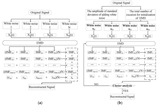
Figure 1.
The flow chart of ensemble empirical mode decomposition (EEMD) and improved ensemble empirical mode decomposition (IEEMD): (a) EEMD and (b) IEEMD.
Figure 1 has shown that the crucial point for EEMD to lessen the mode-mixing problem is that the number of IMF of different signal decomposed by EMD must be equal. However, it is difficult to ensure the same IMF number when the signal with different series of noise is decomposed by EMD in each period. For the proposed IEEMD method, the mode-mixing problem that the oscillations of very disparate amplitude appear in a mode is improved by taking advantage of the uniformity of the white noise probability density function. The other mode-mixing problem where oscillations or frequencies with the same time scale are assigned to different estimated modes, is improved by the cluster analysis.
2.3. Testing and Verification
In this section, a synthetic signal will be used to test and verify the advantage of the IEEMD method when compared with the EEMD method. The noisy signal from the bridge structures is simulated as follows.
where two cosine signals with center frequency 1 Hz and 5 Hz stand for the “true” signals, which contain the structural dynamical information. models the monitoring noise with a signal-to-noise ration [32] 2.66, and a peak signal to noise ration [32] 15.95. The sampling frequency is 256 Hz and the sampling period is 10 s.
The decomposition results are shown in Figure 2.
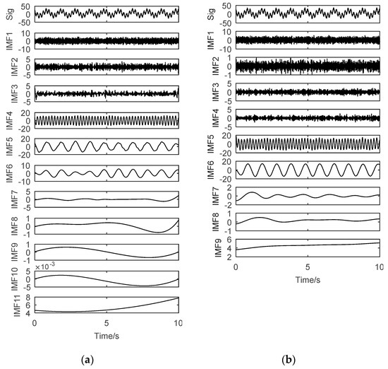
Figure 2.
Intrinsic mode functions (IMFs) decomposed by EEMD and IEEMD. (a) EEMD. (b) IEEMD.
Figure 2 has clearly shown that the number of IMFs decomposed by EEMD is 11, which is two more than the IEEMD. By using EEMD, the frequency of IMF4 is 1 Hz. However, the IMF5 and IMF6 both have 5 Hz frequency components, which indicates that different IMFs contain the same frequency components, and the mode mixing problem still exists. By contrast, by using IEEMD presented in this paper, it can be seen clearly that IMF5 and IMF6 are the main frequency components. The frequency of IMF5 is 1 Hz, and the frequency of IMF6 is 5 Hz. The IEEMD method effectively alleviates the mode-mixing issues.
The decomposition error is compared by superimposing all the decomposed IMFs and comparing them with the original signal. The reconstruction error of the two methods is shown in Figure 3. From Figure 3, it can be seen clearly that the error of IEEMD is in the order of 10−13 and that EEMD is in the order of 1. Clearly, the decomposition accuracy of IEEMD is much higher than that of the original EEMD method.

Figure 3.
Reconstruction error of the simulation signal.
3. Data-Driven Recurrence Quantification Analysis (RQA)
3.1. Brief Description on Recurrence Plot (RP) and RQA
Recurrence plot (RP) measure recurrences of a trajectory in its m-dimensional phase space by the recurrence matrix R, which is defined as the equation below [33].
where N is the number of measured points, is a recurrence threshold distance, is the Heaviside function, and is a norm. Then, if the states of the system at time and that at time are in an -neighborhood, and otherwise. The phase space trajectory is reconstructed from a time series by time delay embedding [33].
where m is the embedding dimension and is the time delay.
The RP is obtained by plotting the recurrence matrix R in its binary entries: a black dot if (recurrence) and a white dot if (no recurrence). Thus, by the definition of R, the RP has a black main diagonal line and is symmetric with respect to the main diagonal [33].
Since the initial purpose of RP was to visualize trajectories in the phase space, the interpretation of RP is qualitative and subjective. Therefore, it lacks quantitative standards [1]. Hence, a quantification of the obtained structures of RP is necessary for a more objective investigation of the considered system. To this end, the recurrence quantification analysis (RQA) was proposed as a quantitative description of RP by Marwan et al. [34], Zbilut et al. [35], and Webber et al. [36] whose diagonal and vertical lines are the base [37]. Furthermore, the RQA can provide information about different characteristics of the RP and can be used to detect transitions in dynamical systems. The RQA measures, which are adopted in this paper, are as follows:
Recurrence rate, RR, is a measure of the density of recurrence points in the RP [37].
where is the recurrence matrix defined in Equation (13) and the main diagonal (i = j) is usually excluded. The RR can be used to reveal changes in dynamic systems.
Determinism, DET, is the ratio of recurrence points that form diagonal structures of at least length to all recurrence points [37].
where is the histogram of diagonal lines of length l given the threshold . Processes with uncorrelated or weakly correlated, stochastic or chaotic behavior cause none or very short diagonals, whereas deterministic processes cause longer diagonals and less single, isolated recurrence points. Therefore, the DET provides a measure for determinism or predictability of the system.
Average diagonal line length, L, is the average time that two segments of the trajectory are close to each other [37].
This can be interpreted as the mean prediction time.
Longest diagonal line, , is related to the exponential divergence of the phase space trajectory [37].
where is the total number of diagonal lines. The faster the trajectory segments diverge, the lower the will be. Analogously to , the maximal length of the vertical lines, , in the RP can be regarded as [37] the following equation.
where is the absolute number of vertical lines.
Entropy, ENTR, refers to the Shannon entropy of the probability to find a diagonal line of exactly length l in the RP [37].
ENTR reflects the complexity of the RP with respect to the diagonal lines. Therefore, for uncorrelated noise, the value of ENTR is rather small, which indicates its low complexity.
Laminarity, LAM, is the ratio between the recurrence points forming the vertical structures and the entire set of recurrence points [37].
Its definition is analogous to the DET in Equation (19), which represents the occurrence of laminar states in the system without describing the length of these laminar phases.
Analogously to ENTR, a new RQA measure, the Entropy of vertical lines (VENTR) is defined in this paper.
where . is the histogram of vertical lines of length v given the threshold .
3.2. Data-Driven RQA
The synchronization analysis is usually used to detect the transitions of different complex systems. The basic types of synchronization in coupled complex systems may be broadly divided into three categories [38]: completely synchronization, generalized synchronization, and phase synchronization. In this section, the relationship between recurrences and phase synchronization of complex systems will be adopted. If two systems synchronize in the same way, their recurrences in phase space are not independent from each other. Hence, by comparing the recurrences of each single system with RQA, some statistical indications about their synchronization type and degree will be set up and tested.
3.2.1. Improved RQA Method
RQA is very sensitive in detecting any dynamic change. However, it can be easily influenced by the value of the setup parameters. One crucial parameter of an RP is the Euclidean distance threshold ε. Too small value of ε may result in quantification of much noise and a very low recurrence rate, which leads to the loss of recurrence information of the underlying system. While, on the other hand, too large values of ε may produce false recurrences or saturate the measurement, which leads to many artefacts [1]. Inspired by the DVV method [39] and the DVRQA method [40], an improved RQA method is proposed here to solve the difficulty of adaptive determination of the Euclidean distance threshold. The basic process is as follows.
- Set the initial value of recurrence threshold and target recurrence rate vector , the value of can be set up based on the equation [39]: , where is a delay matrix consisting of embedding the dimension and delay time.
- Set and construct a recurrence matrix based on Equation (16). Obtain the value based on Equation (18).
- If and satisfy the set tolerance, record the target threshold value . If not, the solution process is performed iteratively until the allowable error is satisfied.
- Repeat step 2 and step 3 until the threshold vector corresponding to is obtained.
- According to every value of , the RQA is performed to obtain the RQA measure vector .
The flow chart of the previously mentioned Improved-RQA method is shown in Figure 4.

Figure 4.
Flow chart of improved - recurrence quantification analysis (RQA) method.
3.2.2. Selection of Other RQA Parameters and Surrogate Techniques
Generally, the mutual information (MI) function [41] and false nearest neighbors (FNN) [41] method are common and robust tools to, respectively, decide the appropriate time delay and embedding dimension . In this paper, the reasonable value for is decided based on the first local minimum of the time-delayed mutual information and the selection of the minimum embedding dimension m, which is based on the false nearest neighbor algorithm proposed in Reference [42].
Theiler et al. [43] introduced the concept of “surrogate data,” which has been extensively used in the context of statistical non-stationary and non-linearity testing. A surrogate time series is generated as a realization of the null hypothesis under study. Thus, given an original signal, realizations of this data must be generated by modifying only the desired characteristic of the signal that is being tested while the rest of the characteristics remain the same. In this paper, the classic Fourier-based technique [44] and the iAAFT (Iterative Amplitude Adjusted Fourier Transform, iAAFT) technique [44] for the nonstationary and nonlinearity generation of surrogates that will be used later in a statistical analysis based on RQA.
3.2.3. The Statistical RQA Measures
The statistical RQA measures proposed in this case are based on the computation of an ensemble of surrogates, which are representative stationary and linear realizations of the null hypothesis. A statistical measure is computed for the original given time series and the surrogates. If the statistic is significantly different from the values obtained for the surrogate set, the null hypothesis can be rejected. The details of the analysis process is as follows.
- The stationary surrogate technique and linear surrogate technique are adopted separately to generate N groups of stationary and linear surrogate signals.
- Improved-RQA is carried out for each group of stationary and linear signals and the RQA measure matrix corresponding to the target recurrence rate are obtained. Each column of the RQA measure matrix represents a set of index vectors of the surrogate signals.
- Calculate the mean and the variance of the RQA measures to obtain the non-stationarity testing and nonlinearity testing confidence interval , .
- Improved-RQA analysis is carried out for the original given signal. Considering the strong noise test environment of the bridge structure, the noise influence factor is introduced to avoid the strong noise submerging the signal and cover up of the real recursive topology of the signal. The mathematical expression of the RQA measures is as follows.where is the noise influence factor. if the given signal is pure. Otherwise, is selected according to the SNR level.
- If each element of the given signal is within the confidence interval, the null hypothesis will be accepted. The nonstationary element and the nonlinear element . Otherwise, , . Let the total size of the RQAs be N , the number of the nonstationary elements and nonlinear elements, which are within the confidence interval, be ,. When the ratios of , are greater than the threshold , the null hypothesis is accepted. Otherwise, the null hypothesis is rejected. Let the binary non-stationarity statistical RQA measure be SNS and nonlinearity statistical RQA measure index be SNL. SNS and SNL can be calculated as follows.
- Let the median value of RQAs be RQAm, then the element pair (RQAm,SNS) and (RQAm,SNL) will be set up as the statistical nonstationary and nonlinear test measures.
The flow chart of the data-driven RQA algorithm is shown in Figure 5.
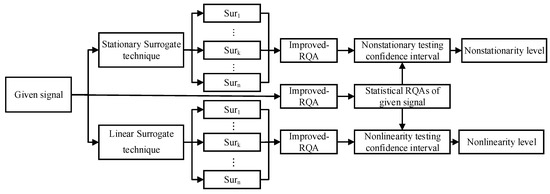
Figure 5.
A data-driven RQA framework for nonstationary and nonlinear signal testing.
4. Multiscale Recurrence Analysis of a Model Cable-Stayed Bridge
Test Description
A 1:20 scale model cable-stayed bridge subjected to dynamic tests will be taken as the case study for the validation of the proposed algorithm in this section. The model bridge, which is shown in Figure 6, may consist of five spans based on the arrangement of the location of towers and piers. The span lengths in this context are: 2.45 m + 4.05 m + 14.24 m + 4.05 m + 2.45 m, which gives the bridge a total length of 27.24 m.
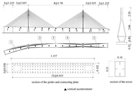
Figure 6.
A model cable-stayed bridge (unit: m).
The superstructure of the model bridge is constructed of a steel -shaped girder with box cross-section on both sides of the girder. The width of the girder is 1.1 m and the height of the girder is 0.081 m. The superstructure is divided into six sections, which are made separately and connected by connecting plates which are numbered inside a circle in the figure, e.g., ①, ②, etc. The superstructure is supported by 60 pairs (or 120 in total) of stay-cables, which are fabricated from wire-ropes of 10 mm diameter and are anchored to the top of the tower. The tower is constructed of two rectangular (0.21 m × 0.14 m) hollow steel columns with wall thickness of 8 mm, which stands 5.95 m in height above the footing. Three cross-beams connect the columns at each tower. The two upper cross-beams are at spacing of 0.34 m center-to-center at the top, and the lower cross-beam is at spacing of 1.397 m center-to-center at the columns. The end spans of the superstructure are supported by four piers. The towers and superstructure are constructed of steel plate, with a yield strength of MPa. The piers are constructed of concrete, with a compressive strength of MPa.
Dynamic properties of the model cable-stayed bridge are characterized by uni-directional piezoelectric accelerometers, which have a sensitivity of 2500 mv/g and an operating frequency in the range of 0.05 to 300 Hz. The arrangement of accelerometers is shown in Figure 6, where 13 solid triangles have been used to denote the location of the vertical accelerometers mounted on the girders. Pulse excitation at the location of the middle span is used to characterize the dynamic properties of the bridge. The damped acceleration attenuation responses of the girder are measured by 13 vertical accelerometers. Different damage locations of the girder is modeled by loosening the bottom bolts of the connecting plate, as shown in Figure 7b. The cable damage is modeled by uninstalling the stay cable, as shown in Figure 7c. In this paper, the responses measured from the girder corresponding to the damage of the connecting plate ② are used to verify the proposed algorithm.
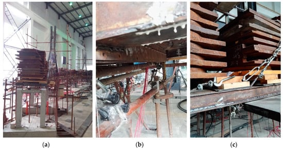
Figure 7.
Photographs of the model cable-stayed bridge: (a) general view of the model bridge, (b) damage of the connecting plate, and (c) damage of the stay-cable.
5. Results and Discussions
The response measured from the number 6 accelerometer under damage conditions of the connecting plate ② is used as an example to show the analysis process. The acceleration waveform in the time domain is shown in Figure 8.
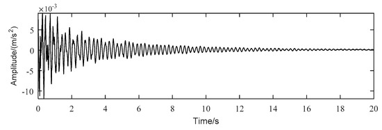
Figure 8.
The measured acceleration waveform.
The IMFs of the given signal can be obtained by using the IEEMD method proposed in Section 2.2, which is shown in Figure 9.
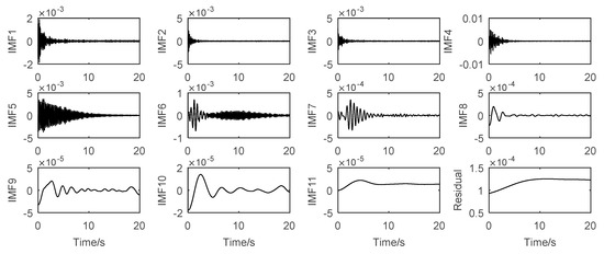
Figure 9.
The extracted IMFs and residual of the selected signal.
The stationary and linear surrogate signals of each IMF can be generated by using the method in Section 3.2.2, which are shown in Figure 10 and Figure 11.
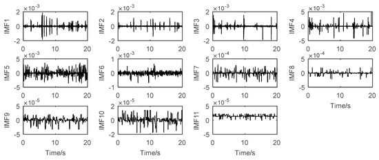
Figure 10.
The stationary surrogate signals of each IMF.
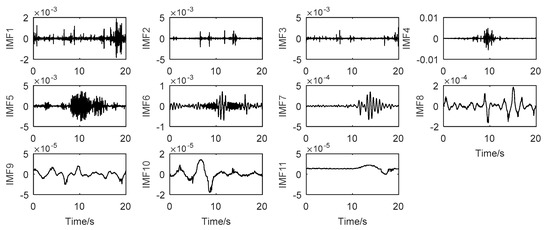
Figure 11.
The linear surrogate signals of each IMF.
The appropriate time delay and embedding dimension of each IMF can be obtained by using the method explained in Section 3.2.2. The mutual information, false nearest neighbors, and phase-space figures of IMF1 are shown in Figure 12. From the figure, we can see that the first local minimum of the time-delayed mutual information is ( is the Sampling interval) and the false nearest neighbors equal zero when the embedding dimension is 7. The appropriate time delay and embedding dimension of other IMFs is similar to the analysis process of the IMF1. The appropriate time delay and embedding dimension parameters of all IMFs are listed in Table 1.
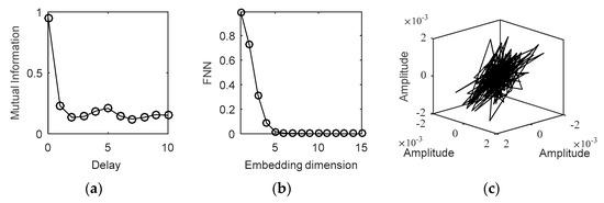
Figure 12.
The time delay, embedding dimension, and phase space of IMF1: (a) Time delay. (b) Embedding dimension. (c) Phase space.

Table 1.
The appropriate time delay and embedding dimension of IMFs.
Eckmann [33] and Marwan [1] both have stated that the length of the diagonal lines is related to the largest positive Lyapunov exponent, which is usually taken as an indication that the system is chaotic and nonlinear. In addition, the length of vertical lines allows for the investigation of intermittency, even for rather short and non-stationary data series [1]. According to this point, in this paper, the diagonal line-based RQA measures (e.g., Lmax, ENTR, DET) are used as indicators of the nonlinear level. The vertical line-based RQA measures (e.g., Vmax, VENTR, LAM) are used as the indicators of the nonstationary level. The statistical six indicators of each IMF can be calculated by using the method described in Section 3.2.3. Due to the length of the paper, we only select the statistical RQA measures of the IMF1 and IMF7 to compare the results, which are shown in Figure 13.
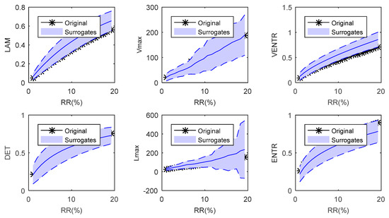
Figure 13.
The statistical RQA index of IMF1.
From Figure 13 and Figure 14, it can be clearly seen that the nonstationary indicators (Vmax, VENTR, LAM) and the nonlinear indicators (Lmax, ENTR, DET) of IMF1 are all in the confidence interval, which indicates that the stationary and linear hypothesis should be accepted. However, the nonstationary indicators and nonlinear indicators of IMF7 all fall outside the confidence interval, which indicates that the stationary and linear hypothesis should be rejected. The conclusion in this case is consistent with the results shown in Figure 9 in which IMF1 mostly contains the stationary and linear white noise, and IMF7 mostly contains the non-stationary and nonlinear structural dynamic information.
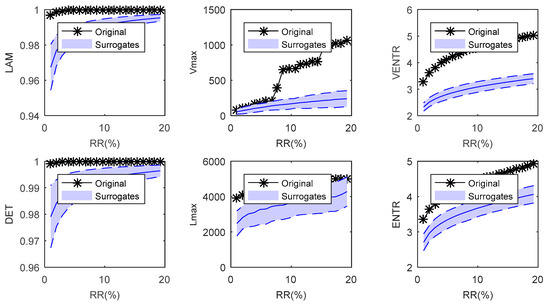
Figure 14.
The statistical RQA index of IMF7.
To further prove the effectiveness of the above nonstationary indicators, the time-frequency analysis of IMF1 and IMF7 is performed by the continuous wavelet transform algorithm [45], which is shown in Figure 15. The figure has shown that the IMF1 has a relatively uniform frequency distribution with time. Unlike the former, the frequency range 1–2 Hz of IMF7 is the major frequency components and the main frequency in IMF7 is steadily decreasing with time. The time-frequency analysis results of IMF1 and IMF7 indicate that the IMF1 is stationary and IMF7 is nonstationary, which are consistent with the results of the proposed nonstationary test indicators in this paper.
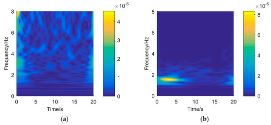
Figure 15.
Time-frequency diagram of IMF1 and IMF7: (a) IMF1. (b) IMF7.
The bispectrum-based method [46] is used to test for linearity of IMF1 and IMF7, which can further prove the effectiveness of the above nonlinear indicators. The bi-spectrum-based test results are shown in Figure 16. The figure has shown that the estimated (full line) and theoretical (dashed line) values of R, the interquartile range of the estimated bi-coherence values, are very close, which indicates that the test of IMF1 show strong evidence of linearity. Contrary to the former, the estimated and theoretical values of R of IMF7 are clearly different and the estimated value is large, which indicates that the test of IMF7 show strong evidence of nonlinearity. The results are consistent with that of the proposed nonlinear test indicators in this paper.

Figure 16.
The interquartile range of the estimated bi-coherence values of IMF1 and IMF7: (a) IMF1. (b) IMF7.
The analysis process has repeated for other IMFs, and the statistical nonstationary and nonlinear RQA measures pairs of all IMFs have been listed in Table 2. In the table, refers to the median value of the statistical RQA measures. refers to the binary statistical RQA measures index.

Table 2.
The statistical RQA measures of IMFs.
From Table 2, it can be clearly seen that the binary statistical RQA measures of IMF1~IMF2 are zero and that of IMF3~IMF11 are one, which indicates that IMF1~IMF2 are linear and stationary and IMF3~IMF11 are nonlinear and non-stationary. To prove the correctness of the conclusion based on binary statistical RQA measures, the energy [47] of each IMF is calculated, which is shown in Figure 17.
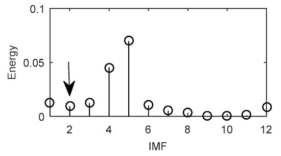
Figure 17.
The IMFs energy of the given signal.
According to References [24,47], the first group of IMFs whose energies are monotonically decreasing can be viewed as white noises. From Figure 17, it can be clearly seen that the first groups of IMFs, which can be regarded as noises are IMF1~IMF2. In addition, it has become a consensus that white Gaussian noise is stationary and linear, which is identical with the conclusion based on the binary statistical RQA measures index proposed in this paper.
The RQA measures median value and statistical RQA measure index of each IMF are shown in Figure 18. The left Y-axis refers to the median value of each RQA measure and the right Y-axis refers to the statistical RQA index. The Y-axis headings have the same meaning as Table 2.
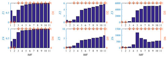
Figure 18.
The statistical RQA measures of each IMF.
Figure 18 shows that the vibration signal monitored from the model bridge has nonstationary and nonlinear components. IMF1 and IMF2 are stationary and linear and IMF3~IMF11 are nonstationary and nonlinear. The median value of statistical RQA measures indicate the nonstationary and nonlinear level of IMF3~IMF11. The nonstationary level and nonlinear level of IMF3~IMF4 are weak, and the nonstationary level and nonlinear level of IMF5~IMF11 are strong. With the increase of IMF, the level of non-linearity and non-stationarity increases, which indicates that apparent dynamics of the considered data are mainly controlled by its medium-frequency and low- frequency components. The conclusion happens to be consistent with that of Reference [19]. It is worth noting that the previously mentioned law cannot be obtained only according to the single RQA measure.
On the basis of the nonlinear and non-stationary test of the model bridge vibration signal, the time-varying dynamical characteristics of the model bridge are studied further. The identification of the time-varying frequency damping ratio has been conducted by using the stochastic subspace identification method with a sliding window technique [48], and the results are shown in Figure 19.
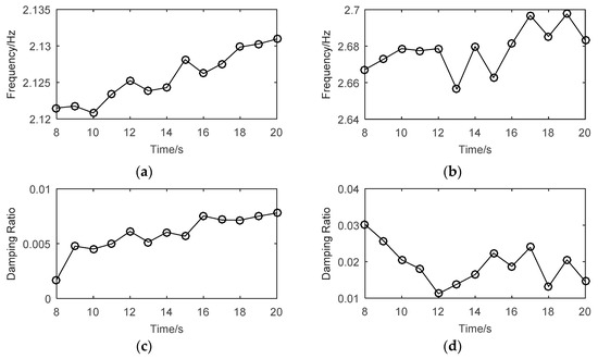
Figure 19.
Time-varying diagram of the first two-order frequency, damping ratio of the curved cable-stayed model bridge: (a) first order, (b) second order, (c) first order, and (d) second order.
Figure 19 has shown that the first two-order frequency and damping ratio of the model bridge are gradually rising with a zigzag line, which indicates obvious time-varying characteristics, and the model bridge system is nonstationary and nonlinear. It is remarkable that the time-varying dynamic information will be lost if the non-stationarity and nonlinearity of the signal is not considered.
6. Conclusions
Nonlinear and non-stationary detection of complex signals is usually a prerequisite for further developing time-varying system identification methods. In this paper, the framework of the combination of signal decomposition methods with statistical RP and RQA is adopted to solve the difficulty of original RP’s application in bridge engineering. The following concluding remarks can be drawn from this study.
1. By introducing a new white noise assistance way by considering the uniformity of white noise probability density function, and cluster analysis to original EEMD, an improved EEMD method is proposed to alleviate the mode mixing issues of the EEMD method. The decomposition and reconstruction of a numerical simulation signal has proven the superiority of IEEMD.
2. By combining the surrogate techniques and hypothesis-testing scheme of nonstationary and nonlinear synchronization, a data-driven RQA method is performed on the single-mode signal components and the true indicator pairs, which contain the statistical RQA measures median and a binary RQA index are set up. The results of the conventional time-frequency analysis method, nonlinear test method, and energy analysis are separately used to prove the effectiveness of the nonstationary, nonlinear RQA measures and binary RQA index. Based on the effective implementation of a model cable-stayed bridge, the frequency-evolving RQA of the given signal indicates that the apparent dynamics are mainly controlled by its medium-frequency and low-frequency components.
Conclusively, although the novel method that combines signal decomposition with statistical RP and RQA was applied to detect the nonlinearity and non-stationarity of signals from a model cable-stayed bridge, this method has the potential to be applied to bridges in real complex operating environment. The difference is that the level of noise contained in those signals is generally high and some effective signal processing technologies such as adaptive noise reduction methods may be needed to improve the SNR.
7. Future Works
In future works, in addition to continuing with the topic, we will: (i) study the method for detecting and repairing the abnormal data in signals, (ii) study the fast RP and RQA algorithm, (iii) try to conduct nonlinear and non-stationary detection on very long time series from the full-scale bridge, and (iv) apply the method proposed in this paper to other structures such as high-rise buildings as well as large and long tunnels.
Author Contributions
Conceptualization, E.Z. and D.S. Funding acquisition, D.S. and Q.L. Investigation, E.Z. Methodology, E.Z. Project administration, D.S. and Q.L. Resources, D.S. Supervision, D.S. and Q.L. Validation, E.Z., D.S., and Q.L. Visualization, E.Z. Writing – original draft, E.Z. Writing – review & editing, E.Z., D.S., and Q.L.
Funding
The National Key R&D Program of China, grant number 2016YFC0802202, the National Science Foundation, grant number 51678489, and the Sichuan Science and Technology Program, grant number 2016JY0130, funded this research.
Conflicts of Interest
The authors declare no conflict of interest.
References
- Chen, Y.; Yang, H. Multiscale recurrence analysis of long-term nonlinear and nonstationary time series. Chaos Solitons Fractals Interdiscip. J. Nonlinear Sci. Nonequilibrium Complex Phenom. 2012, 45, 978–987. [Google Scholar] [CrossRef]
- Nagarajaiah, S.; Erazo, K. Structural monitoring and identification of civil infrastructure in the United States. Struct. Monit. Maint. 2016, 3, 51–69. [Google Scholar] [CrossRef]
- Marwan, N.; Romano, M.C.; Thiel, M.; Kurths, J. Recurrence plots for the analysis of complex systems. Phys. Rep. 2007, 438, 237–329. [Google Scholar] [CrossRef]
- Eckmann, J.P.; Kamphorst, S.O.; Ruelle, D. Recurrence Plots of Dynamical Systems. World Sci. Ser. Nonlinear Sci. Ser. A 1995, 16, 441–446. [Google Scholar]
- Webber, C.L., Jr.; Zbilut, J.P. Recurrence quantifications: Feature extractions from recurrence plots. Int. J. Bifurc. Chaos 2007, 17, 3467–3475. [Google Scholar] [CrossRef]
- Webber, C.L., Jr.; Ioana, C.; Marwan, N. Recurrence Plots and Their Quantifications: Expanding Horizons. In Springer Proceedings in Physics; Springer International Publishing: New York, NY, USA, 2016. [Google Scholar]
- Schinkel, S.; Marwan, N.; Kurths, J. Order patterns recurrence plots in the analysis of ERP data. Cogn. Neurodyn. 2007, 1, 317–325. [Google Scholar] [CrossRef]
- Romano, M.C.; Thiel, M.; Kurths, J.; von Bloh, W. Multivariate recurrence plots. Phys. Lett. A 2004, 330, 214–223. [Google Scholar] [CrossRef]
- Lange, H.; Boese, S. Recurrence Quantification and Recurrence Network Analysis of Global Photosynthetic Activity. In Recurrence Quantification Analysis; Springer International Publishing: New York, NY, USA, 2015; pp. 349–374. [Google Scholar]
- Hoshi, R.A.; Pastre, C.M.; Vanderlei, L.C.M.; Godoy, M.F. Assessment of Heart Rate Complexity Recovery from Maximal Exercise Using Recurrence Quantification Analysis. In Recurrence Plots and Their Quantifications: Expanding Horizons; Springer: Cham, Switzerland, 2016; pp. 157–168. [Google Scholar]
- Hirata, Y.; Oda, A.; Ohta, K.; Aihara, K. Three-dimensional reconstruction of single-cell chromosome structure using recurrence plots. Sci. Rep. 2016, 6, 34982. [Google Scholar] [CrossRef] [PubMed]
- Tibau, E.; Soriano, J. Analysis of spontaneous activity in neuronal cultures through recurrence plots: Impact of varying connectivity. Eur. Phys. J. Spec. Top. 2018, 227, 999–1014. [Google Scholar]
- Bastos, J.A.; Caiado, J. Recurrence quantification analysis of global stock markets. Phys. A Stat. Mech. Appl. 2012, 390, 1315–1325. [Google Scholar] [CrossRef]
- Tzagkarakis, G.; Dionysopoulos, T. Restoring Corrupted Cross-Recurrence Plots Using Matrix Completion: Application on the Time-Synchronization between Market and Volatility Indexes. In Recurrence Plots and Their Quantifications: Expanding Horizons; Springer: Cham, Switzerland, 2016; pp. 241–263. [Google Scholar]
- Garcia-Ochoa, E.; Corvo, F. Using recurrence plot to study the dynamics of reinforcement steel corrosion. Prot. Met. Phys. Chem. Surf. 2015, 51, 716–724. [Google Scholar] [CrossRef]
- Savari, C.; Kulah, G.; Koksal, M.; Sotudeh-Gharebagh, R.; Zarghami, R.; Mostoufi, N. Monitoring of liquid sprayed conical spouted beds by recurrence plots. Powder Technol. 2017, 316, 148–156. [Google Scholar] [CrossRef]
- Yang, D.; Ren, W.X.; Hu, Y.D.; Li, D. Selection of optimal threshold to construct recurrence plot for structural operational vibration measurements. J. Sound Vib. 2015, 349, 361–374. [Google Scholar] [CrossRef]
- Kecik, K.; Ciecielag, K.; Zaleski, K. Damage detection of composite milling process by recurrence plots and quantifications analysis. Int. J. Adv. Manuf. Technol. 2017, 89, 133–144. [Google Scholar] [CrossRef]
- Zbilut, J.P.; Webber, C.L., Jr. Recurrence Quantification Analysis. In Wiley Encyclopedia of Biomedical Engineering; John Wiley & Sons, Inc.: Hoboken, NJ, USA, 2006. [Google Scholar]
- Catone, M.C.; Faggini, M. Recurrence Analysis: Method and Applications. In Data Science and Social Research; Springer International Publishing: New York, NY, USA, ; 2017. [Google Scholar]
- Amezquita-Sanchez, J.P.; Adeli, H. Signal processing techniques for vibration-based health monitoring of smart structures. Arch. Comput. Methods Eng. 2016, 23, 1–15. [Google Scholar] [CrossRef]
- Ding, H.; Crozier, S.; Wilson, S. Optimization of Euclidean distance threshold in the application of recurrence quantification analysis to heart rate variability studies. Chaos Solitons Fractals 2008, 38, 1457–1467. [Google Scholar] [CrossRef]
- Beim Graben, P.; Sellers, K.K.; Fröhlich, F.; Hutt, A. Optimal estimation of recurrence structures from time series. Europhys. Lett. 2016, 114, 38003. [Google Scholar] [CrossRef]
- Xiong, H.; Shang, P.; Bian, S. Detecting intrinsic dynamics of traffic flow with recurrence analysis and empirical mode decomposition. Phys. A Stat. Mech. Appl. 2017, 474, 70–84. [Google Scholar] [CrossRef]
- Gao, Q.; Li, G.X.; Tian, X.; Sun, J. A novel traffic prediction method based on IMF. In Advanced Materials Research; Trans Tech Publications: Zurich, Switzerland, 2012; Volume 490, pp. 1421–1425. [Google Scholar]
- Yan, R.; Chen, X.; Mukhopadhyay, S.C. Advanced Signal Processing for Structural Health Monitoring. In Structural Health Monitoring; Springer: Cham, Switzerland, 2017; pp. 1–11. [Google Scholar]
- Liu, T.; Luo, Z.; Huang, J.; Yan, S. A Comparative Study of Four Kinds of Adaptive Decomposition Algorithms and Their Applications. Sensors 2018, 18, 2120. [Google Scholar] [CrossRef]
- Wu, Z.; Huang, N.E. Ensemble Empirical Mode Decomposition: A Noise-Assisted Data Analysis Method. Adv. Adapt. Data Anal. 2009, 1, 1–41. [Google Scholar] [CrossRef]
- Keylock, C.J. Multifractal surrogate-data generation algorithm that preserves pointwise Hölder regularity structure, with initial applications to turbulence. Phys. Rev. E 2017, 95, 032123. [Google Scholar] [CrossRef]
- SHAN, D.; LI, Q.; KHAN, I. Adaptive Signal Decomposition and Reconstruction for Bridge Structural Dynamic Testing. In IABSE Symposium Report; International Association for Bridge and Structural Engineering: Zurich, Switzerland, 2016; Volume 106, pp. 415–423. [Google Scholar]
- Huang, N.E.; Shen, S.S.P. Hilbert-Huang transform and its applications. In Hilbert-Huang Transform and Its Applications; World Scientific: Singapore city, Singapore, 2005. [Google Scholar]
- Rabie, T. Robust Estimation Approach for Blind Denoising; IEEE Press: Piscataway, NJ, USA, 2005. [Google Scholar]
- Eckmann, J.P.; Kamphorst, S.O.; Ruelle, D. Recurrence Plots of Dynamical Systems. Europhys. Lett. 1987, 4, 973–977. [Google Scholar] [CrossRef]
- Marwan, N.; Wessel, N.; Meyerfeldt, U.; Kurths, J. Recurrence-plot-based measures of complexity and their application to heart-rate-variability data. Phys. Rev. E 2002, 66, 026702. [Google Scholar] [CrossRef] [PubMed]
- Zbilut, J.P.; Webber, C.L., Jr. Embeddings and delays as derived from quantification of recurrence plots. Phys. Lett. A 1992, 171, 199–203. [Google Scholar] [CrossRef]
- Webber, C.L., Jr.; Zbilut, J.P. Dynamical assessment of physiological systems and states using recurrence plot strategies. J. Appl. Physiol. 1994, 76, 965–973. [Google Scholar] [CrossRef] [PubMed]
- Zbilut, J.P.; Giuliani, A.; Webber, C.L., Jr. Recurrence quantification analysis and principal components in the detection of short complex signals. Phys. Lett. A 1998, 237, 131–135. [Google Scholar] [CrossRef]
- Strogatz, S. Synchronization: A Universal Concept in Nonlinear Sciences. Phys. Today 2003, 56, 47. [Google Scholar] [CrossRef]
- Gautama, T.; Mandic, D.P.; Van Hulle, M.M. The delay vector variance method for detecting determinism and nonlinearity in time series. Phys. D Nonlinear Phenom. 2004, 190, 167–176. [Google Scholar] [CrossRef]
- Carrión, A.; Miralles, R. New Insights for Testing Linearity and Complexity with Surrogates: A Recurrence Plot Approach. In Recurrence Plots and Their Quantifications: Expanding Horizons; Springer: Cham, Switzerland, 2016; pp. 91–112. [Google Scholar]
- Tong, H. Non-Linear Time Series Analysis; Cambridge University Press: Oxford, UK, 2011. [Google Scholar]
- Kennel, M.B.; Brown, R.; Abarbanel, H.D.I. Determining embedding dimension for phase-space reconstruction using a geometrical construction. Phys. Rev. A 1992, 45, 3403. [Google Scholar] [CrossRef]
- Theiler, J.; Eubank, S.; Longtin, A.; Farmer, J.D. Testing for nonlinearity in time series: The method of surrogate data. Phys. D Nonlinear Phenom. 1992, 58, 77–94. [Google Scholar] [CrossRef]
- Schreiber, T.; Schmitz, A. Surrogate Time Series. Phys. D Nonlinear Phenom. 1999, 142, 346–382. [Google Scholar] [CrossRef]
- Allen, R.L. Signal Analysis: Time, Frequency, Scale, and Structure; IEEE Xplore: Piscataway, NJ, USA, 2004. [Google Scholar]
- Birkelund, Y.; Hanssen, A. Improved bispectrum based tests for Gaussianity and linearity. Signal Process. 2009, 89, 2537–2546. [Google Scholar] [CrossRef]
- Yin, Y.; Shang, P. Multiscale Detrended Cross-Correlation Analysis of Traffic Time Series Based on Empirical Mode Decomposition. Fluct. Noise Lett. 2015, 14, 1550023. [Google Scholar] [CrossRef]
- Inamullah Khan. Long Term Operational Modal Parameter Identification of Long Span Cable Stayed Bridge; Southwest Jiaotong University: Chengdu City, Sichuan Province, China, 2016. [Google Scholar]
© 2019 by the authors. Licensee MDPI, Basel, Switzerland. This article is an open access article distributed under the terms and conditions of the Creative Commons Attribution (CC BY) license (http://creativecommons.org/licenses/by/4.0/).