Dynamic Parameter Identification of a Long-Span Arch Bridge Based on GNSS-RTK Combined with CEEMDAN-WP Analysis

Abstract

Under the action of wind, traffic, and other influences, long-span bridges are prone to large deformation, resulting in instability and even destruction. To investigate the dynamic characteristics of a long-span concrete-filled steel tubular arch bridge, we chose a global navigation satellite systems-real-time kinematic (GNSS-RTK) to monitor its vibration responses under ambient excitation. A novel approach, the use of complete ensemble empirical mode decomposition with adaptive noise combined with wavelet packet (CEEMDAN-WP) is proposed in this study to increase the accuracy of the signal collected by GNSS-RTK. Fast Fourier transform (FFT) and random decrement technique (RDT) were adopted to calculate structural modal parameters. To verify the combined denoising and modal parameter identification methods proposed in this paper, we established the structural finite element model (FEM) for comparison. Through simulation and comparison, we were able to draw the following conclusions. (1) GNSS-RTK can be used to monitor the dynamic response of long-span bridges under ambient excitation; (2) the CEEMDAN-WP is an efficient method used for the noise reduction of GNSS-RTK signals; (3) after signal filtering and noise reduction, structural modal parameters are successfully derived through RDT and illustrated graphically; and (4) the first-order natural frequency identified by field measurement is slightly higher than the FEM in this work, which may have been caused by bridge damage or the inadequate accuracy of the finite element model.

1. Introduction

Nowadays, with the development of new materials and high-tech solutions, an increasing number of long-span bridges have emerged. Due to the influences of traffic, wind, corrosion, tidal currents, and the combination of these, these bridges easily succumb to large deformation or even destruction. Natural frequency, mode shape, and damping ratio are basic dynamic characteristics of civil engineering structures, which can reflect structures’ security and stability and are worthy of further research. Recent developments in field measurement techniques have provided rapid acquisition of data and highly reliable results for analyzing structural dynamic responses.

Accelerometer monitoring is an effective means with which to monitor the dynamic characteristics of long-span bridges [1,2]. However, it inevitably causes drift errors as it requires a double integral for acquiring deformation displacement [3,4]. Global positioning system (GPS) has been proven a useful means with which to monitor structural dynamic displacement, which is especially suitable for large scale structures with large deformation and low frequency [5,6,7]. The authors of this paper have performed an in-depth study on this topic [8,9,10]. GPS real-time kinematic (RTK) is the primary method used for monitoring structural continuous dynamic deformation [11]. Compared to GPS-RTK, multiconstellation GNSS-RTK can accept GPS, GLONASS, and BeiDou navigation satellite system (BDS) satellite signals at the same time. Its number of visible satellites of the multiconstellation GNSS system is significantly increased, and the position dilution of precision (PDOP) value is clearly decreased [12]. Considering the advantages of the multiconstellation GNSS-RTK system, it was adopted to monitor the dynamic deformation of a long-span concrete filled steel tubular arch bridge in this study.

There are two critical factors in the large-scale structural health monitoring field. One is the selection of sensors and the other is the signal processing method. It has been noted that the positioning accuracies of RTK-GNSS sensors are limited, i.e., in the horizontal direction: ±1 cm; in the vertical direction: ±2 cm. In this paper, we have mainly focused on researching structural vertical vibration, and thus a proper denoising method is needed to ensure monitoring accuracy. Empirical mode decomposition (EMD) [13] is an efficient means of processing nonlinear and nonstationary signals, and decomposes signals into a number of monochromatic intrinsic mode functions (IMFs). After the EMD process, there may be mode mixing in IMFs. A novel method called ensemble empirical mode decomposition (EEMD) has been proposed to alleviate this problem [14]. At the core of the EEMD method is the addition of white noise. In this way, the mode mixing problem is alleviated. However, this creates new problems. The additional white noise is not able to be completely removed, and the interactions between signal and noise will bring different modes. To overcome these situations, the complementary ensemble empirical mode decomposition (CEEMD) method was developed [15]. By adding positive and negative white noise into the signal, the reconstruction error caused by the white noise can be reduced and the computational efficiency is increased. Nevertheless, this method cannot solve the problem of the additional mode caused by adding different noise signals. Thus, the complete ensemble empirical mode decomposition with adaptive noise (CEEMDAN) method was introduced [16]. This method realizes an accurate reconstruction of the decomposed signal and solves the additional mode problem. Additionally, a few novel EMD methods have been proposed in recent years (e.g., the step-by-step EMD method [17,18] and the wavelet-bounded EMD method [19,20]). Just as in EMD, the traditional wavelet is another efficient technique and has been widely applied in signal processing domain [21,22,23,24,25]. The wavelet packet (WP) is a popularization of the traditional wavelet, which can divide the frequency domain adaptively [26]. There has been much research performed on structural vibration response analysis based on the WP technique [27,28,29,30]. Typically, the structural vibration response signal is mixed in with a lot of noise and WP is an efficient way to deal with the white noise. To improve the denoising effects of the GNSS-RTK signal, we propose a two-step denoising method, which integrates the merits of both CEEMDAN and WP and is called CEEMDAN-WP.

Modal parameters identification is an important part of structural health monitoring [31,32]. Structural dynamic deformation monitoring and modal parameter identification under ambient excitation do not need to predict the input signal and do not damage the structure nor affect its normal operation. Simply via the output response can the structural operating modal parameters can be obtained. Cole [33] advanced a modal parameter identification method named the random decrement technique (RDT), which is based on output signals only. In the cases where the ambient excitation is stationary and random, theoretically like white noise, RDT can convert the ambient responses to random decrements [34,35,36]. Recently, RDT has been employed in extracting modal parameters from structural nonstationary response [37,38,39]. Therefore, it may be feasible to employ RDT in structural dynamic characteristics analysis under ambient excitation.

This paper primarily focuses on studying the dynamic response of a long-span concrete-filled steel tubular arch bridge based on the GNSS-RTK technique. Above all, the stability test was conducted to assess the accuracy of GNSS-RTK receivers and, secondly, the FEM of the bridge was established to provide a reference with which to compare the field measurement results. Subsequently, a combined denoising method (CEEMDAN-WP) is proposed in order to process the monitoring signals from the GNSS-RTK receivers. Finally, the structural modal parameters are identified through FFT and RDT.

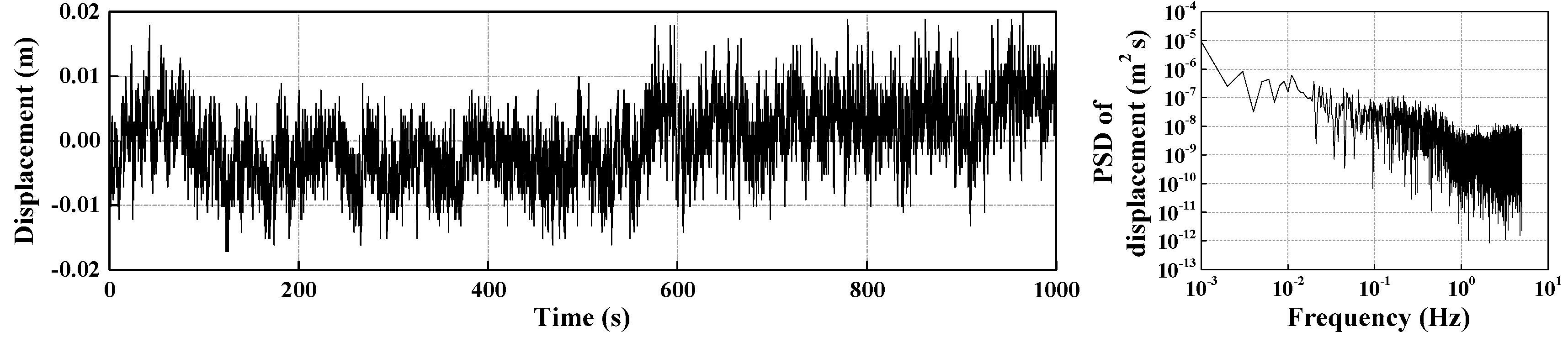
2. Stability Test of GNSS-RTK Receivers

To evaluate the accuracy of the GNSS-RTK receivers, a stability test was implemented in a wide and breezeless site, as shown in Figure 1. There were five Hai-Xingda H32 receivers from Hi-target company in Tianjin, China employed in the experiment. Among those five instruments, one was designed as a reference station, while the other four were rover stations. Each of the rover stations not only received information from the reference station through radio-receiving equipment, but also automatically collected three-dimensional information of measuring points together some systematic errors (e.g., the satellite clock error, receiver clock error, ionospheric and tropospheric refraction errors, etc.). Then, the coordinate values of the measuring points could be obtained through real-time differential processing. This experiment was carried out for three hours without interruption. The sampling rate was set to 10 Hz.

One monitoring point has been selected as an illustrative example; the other points are similar enough to not need repeating. Theoretically, there should not be any amplitude variation of all the monitoring points. However, the monitoring results present violent oscillations due to background noise. Figure 2 presents a captured part of the monitoring data of the vertical displacement. The vibration amplitudes are within ±2 cm, which confirm a standard precision of the GNSS-RTK sensors as mentioned above. The root mean square (RMS) was employed for the assessment of the background noise level of the GNSS-RTK receivers. In this experiment, the RMS result was 0.0058 m, which is small and within a reasonable range. Nevertheless, the structural dynamic deformation in this research was also small. Hence, there should be a further step which considers the background noise mixed in with the GNSS-RTK signal. The power spectral density (PSD) of the monitored data was obtained through FFT. As shown in Figure 2, the low-frequency background noise is less than 0.06 Hz. The spectrum distribution characteristics of high-frequency noise above 0.06 Hz are similar to the characteristics of white noise. The PSD values of high-frequency noise range from 10⁻¹² m² s to 10⁻⁷ m² s. The natural frequency value of the Rainbow Bridge is far greater than 0.06 Hz, and thus the low frequency components less than 0.06 Hz in the measurement signal can be cognized as noise directly. As long as a reasonable threshold value is set, the above cognized noise can be dealt with using traditional denoising algorithms. However, high-frequency random noise, which presents a wide distribution in the frequency domain, is hard to remove. To address this problem, a combined denoising method, which addresses both low-frequency and high-frequency noise, is proposed in the next section.

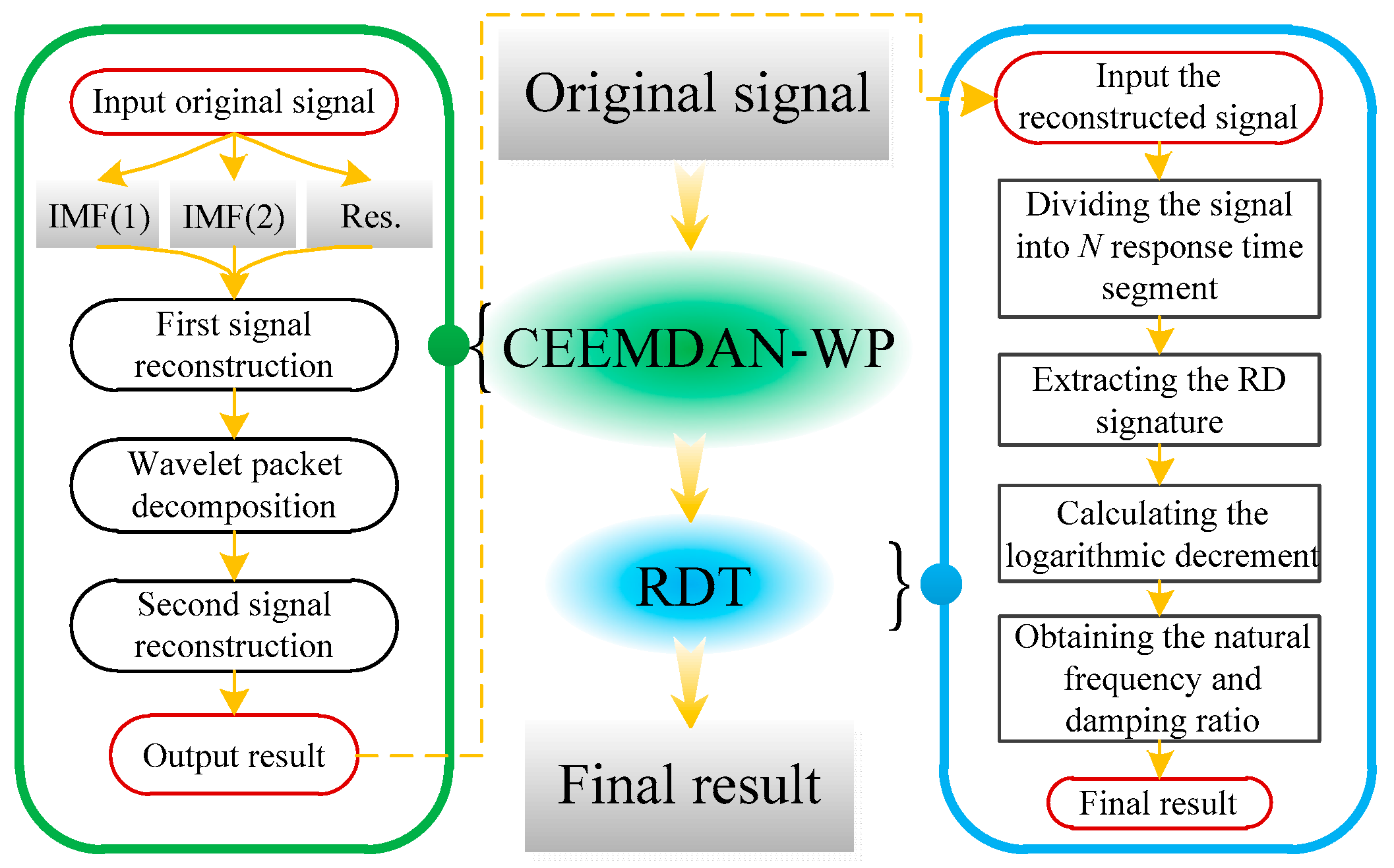
3. The Principle of CEEMDAN-WP and RDT

This section introduces a novel algorithm named CEEMDAN-WP, which integrates the CEEMDAN and wavelet packet decomposition techniques for signal denoising. In addition, RDT and a related technique are proposed for modal identification. A flow chart of signal denoising and modal identification procedures is shown in Figure 3. The specific algorithms of mentioned are introduced in the following subsection.

3.1. EEMD, CEEMD, and CEEMDAN Algorithms

The core of the EMD algorithm is decomposition, through which a number of IMFs can be obtained [13]. The IMF components satisfy two conditions: the number of extreme points and zero-crossing points are equal or at most have a difference of one, and the average of the upper and lower envelopes is zero. Following EMD, EEMD mainly focuses on ameliorating the problem of mode mixing [14]. The EEMD algorithm is presented as follows.

• Add Gauss white noise $\omega \left(t\right)$ into the original signal $x\left(t\right)$ and thus produce a new signal $X\left(t\right)$.

  $$X\left(t\right)=x\left(t\right)+\omega \left(t\right)$$

  (1)
• Using the EMD algorithm, $X\left(t\right)$ is decomposed into a number of IMF components and a residual component $r\left(t\right)$.

  $$X\left(t\right)={\displaystyle \sum _{i=1}^{N}im{f}_i\left(t\right)+r\left(t\right)}$$

  (2)
• By repeating the above two steps, the IMFs $im{f}_{ij}\left(t\right)$ are obtained, where $i$ is the iteration number and $j$ is the mode.
• Compute the average of the IMF components to eliminate the effects of additional white noise.

  $$im{f}_j\left(t\right)=\frac{1}{N}{\displaystyle \sum _{i=1}^{N}im{f}_{ij}\left(t\right)}$$

  (3)

Although EEMD can reduce the influence of mode mixing, the noise remains. To solve this problem, a CEEMD algorithm [15] is introduced, which can be expressed as

• Add positive and negative white noise ${\omega }^{\pm }\left(t\right)$ into the original signal $x\left(t\right)$, and generate two new signals $X^{\pm }\left(t\right)$.

  $$\{\begin{array}{l}{X}^{+}\left(t\right)=x\left(t\right)+{\omega }^{+}\left(t\right)\\ X^{-}\left(t\right)=x\left(t\right)+{\omega }^{-}\left(t\right)\end{array}$$

  (4)
• Repeat the above step, and decompose the new signals using EMD.
• Derive two sets of IMF components for the new signals.
• Calculate decomposition results by averaging multiple components.

  $$im{f}_j\left(t\right)=\frac{1}{2N}{\displaystyle \sum _{i=1}^{2N}im{f}_{ij}\left(t\right)}$$

  (5)

To alleviate the computational load and maintain the ability to eliminate mode mixing, Torres et al. [16] proposed a method (i.e., the CEEMDAN method). This method can be divided into the following steps.

• Define $E_j(\cdot )$ as the operator which produces the $j$-th IMF which has been decomposed based on the EMD algorithm. The first mode $im{f^{\prime }}_1$ is derived by EMD from the signal $x\left(t\right)+{\epsilon }_0{\omega }_i\left(t\right)$.

  $$im{f}_1\left(t\right)=\frac{1}{N}{\displaystyle \sum _{i=1}^{N}im{f}_{i1}\left(t\right)}$$

  (6)

  where ${\epsilon }_0$ is the amplitude of the added white noise and ${\omega }_i\left(t\right)$ is the white noise with unit variance.
• Calculate the first residual signal.

  $$r_1\left(t\right)=x\left(t\right)-im{f^{\prime }}_1\left(t\right)$$

  (7)
• Decompose the signal $r_1\left(t\right)+{\epsilon }_1{E}_1\left({\omega }_i\left(t\right)\right)$ $\left(i=1,\cdots ,N\right)$ to derive the first mode, after which the second mode is defined.

  $$im{f^{\prime }}_2\left(t\right)=\frac{1}{N}{\displaystyle \sum _{i=1}^N{E}_1\left(r_1\left(t\right)+{\epsilon }_1{E}_1\left({\omega }_i\left(t\right)\right)\right)}$$

  (8)
• For $j=2,\cdots ,J$, calculate the $j$-th residual signal.

  $$r_j\left(t\right)=r_{j-1}\left(t\right)-im{f^{\prime }}_j\left(t\right)$$

  (9)
• For $j=2,\cdots ,J$, decompose the signal $r_j\left(t\right)+{\epsilon }_j{E}_j\left({\omega }_i\left(t\right)\right)$ $\left(i=1,\cdots ,N\right)$ to derive the first mode, after which the $\left(j+1\right)$-th mode is defined.

  $$im{f^{\prime }}_{j+1}\left(t\right)=\frac{1}{N}{\displaystyle \sum _{i=1}^N{E}_1\left(r_j\left(t\right)+{\epsilon }_j{E}_j\left({\omega }_i\left(t\right)\right)\right)}$$

  (10)
• Turn to step 4 for the next $j$.

Repeat Steps 4–6 until the residue has no more than two extrema, and satisfy the relationship

$$R\left(t\right)=x\left(t\right)-{\displaystyle \sum _{j=1}^{J}im{f^{\prime }}_j\left(t\right)}$$

(11)

where J is the total number of modes.

Then, the original signal $x\left(t\right)$ is defined as

$$x\left(t\right)={\displaystyle \sum _{j=1}^{J}im{f^{\prime }}_j\left(t\right)}+R\left(t\right)$$

(12)

From Equation (12), the CEEMDAN method can provide a complete and accurate reconstruction signal. Meanwhile, at each stage, noise of different signal noise ratio (SNR) values can be obtained by adjusting the coefficient ${\epsilon }_j$.

3.2. WP Method

WP is a development of the wavelet technique, which can decompose the signal of both low-frequency components and high-frequency components. WP decomposition can be expressed as

$$\{\begin{array}{l}{d}_l^{j,2n}={\displaystyle \sum _k{a}_{k-2l}{d}_k^{j+1,n}}\\ d_l^{j,2n+1}={\displaystyle \sum _k{b}_{k-2l}{d}_k^{j+1,n}}\end{array}$$

(13)

where $d_l^{j,2n}$ and $d_l^{j,2n+1}$ are wavelet packet coefficients and $a_{k-2l}$ and $b_{k-2l}$ are derivatives of filter coefficients.

WP reconstruction can be expressed as

$$d_l^{j+1,n}={\displaystyle \sum _k\left(h_{l-2k}{d}_k^{j,2n}+g_{l-2k}{d}_k^{j,2n+1}\right)}$$

(14)

3.3. The CEEMDAN-WP Model

The combined CEEMDAN-WP model has comprehensive advantages over both the individual CEEMDAN and WP methods. Its specific steps may be presented as follows.

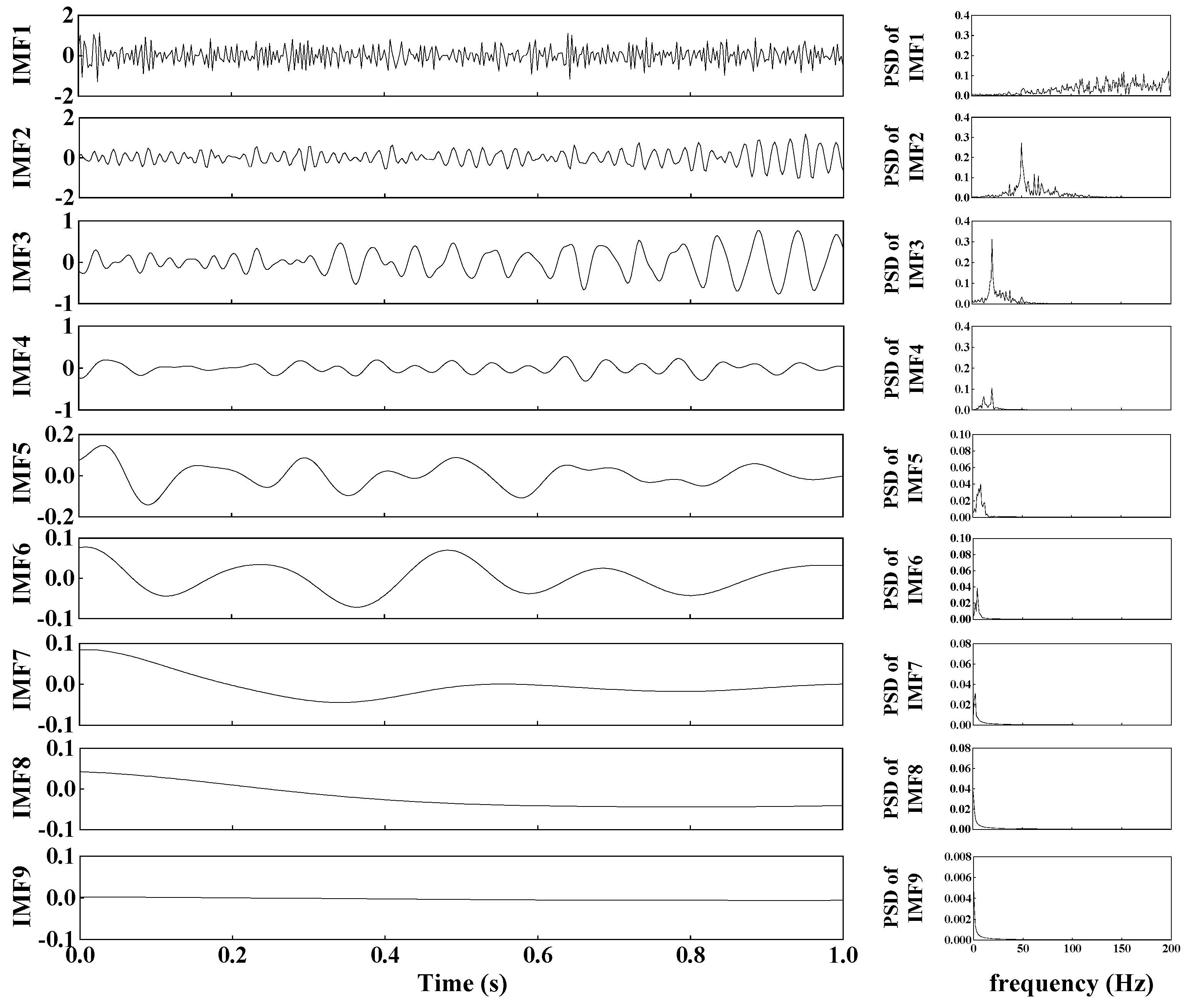
• CEEMDAN is employed for decomposition to obtain a series of IMFs.
• Because of the existence of background noise, some IMF components are noise dominated. Reconstruct signals after removing the components which are noise dominated.
• A three-level WP is used to decompose the signal obtained in Step 2.
• Determine the classic wavelet basis.
• Select proper thresholds and quantify the decomposed coefficients.
• Reconstruct the signal and export.

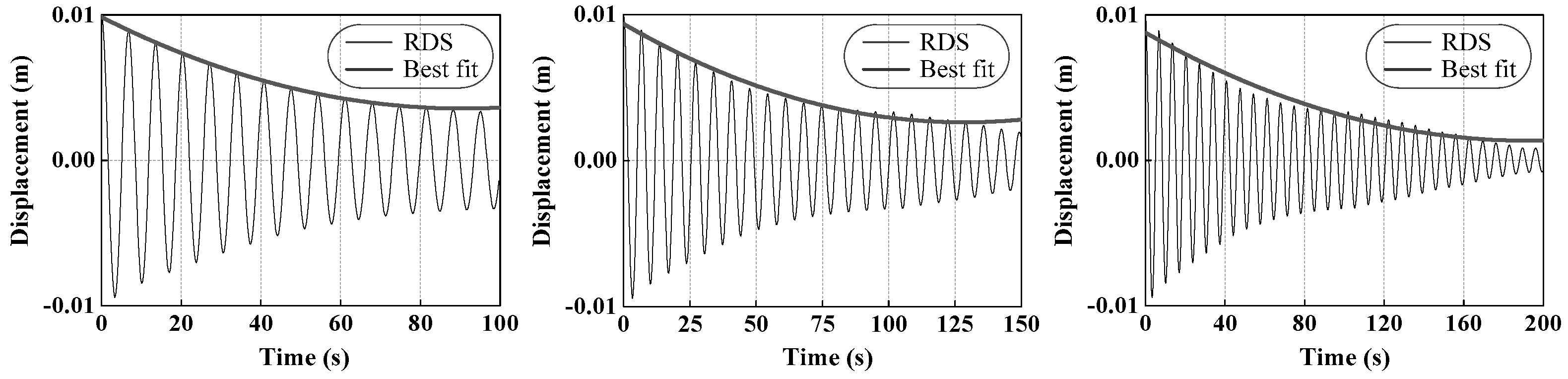
3.4. The RDT Method

RDT is a basic means with which to extract structural free-attenuation vibration signals from random vibration response signals. The extraction is usually regarded as a structural random decrement signature (RDS), which indicates the free vibration of the dynamic system under a supposed stationary random vibration and certain initial conditions [40,41]. In this study, the displacement response signal $x\left(t\right)$ (i.e., Signal R2) is divided into a series of time sample functions $x\left(t_i+\tau \right)$ ($i=1,2,3,\cdot \cdot \cdot ,N$). N is the number of samples and $\tau =t-t_i$. Furthermore, the RDS can be obtained via the average of the time segments $x\left(t_i+\tau \right)$ of the structural response, which can be expressed as

$$R\left(\tau \right)=\frac{1}{N}{\displaystyle \sum _{i=1}^N\left\{x\left(t_i+\tau \right)|x\left(t_i\right)=C\right\}}$$

(15)

where C is the initial condition assumed by $x\left(t\right)$ at time $t_i$.

Based on the RDS, the natural frequency is presented as

$$f=\frac{1}{T}$$

(16)

where T is the measured period of the RDS.

The damping ratio is obtained by a logarithmic decrement approach. The logarithmic decrement $\beta$ can be expressed as

$$\beta =\frac{1}{n}\ln \left|\frac{A_i}{A_{i+n}}\right|$$

(17)

where $A_i$ and $A_{i+n}$ are the amplitudes of cycles $i$ and $i+n$, respectively. Ultimately, the structural damping ratio $\xi$ is derived as

$$\xi =\sqrt{\frac{{\beta }^2}{4{\pi }^2+{\beta }^2}}$$

(18)

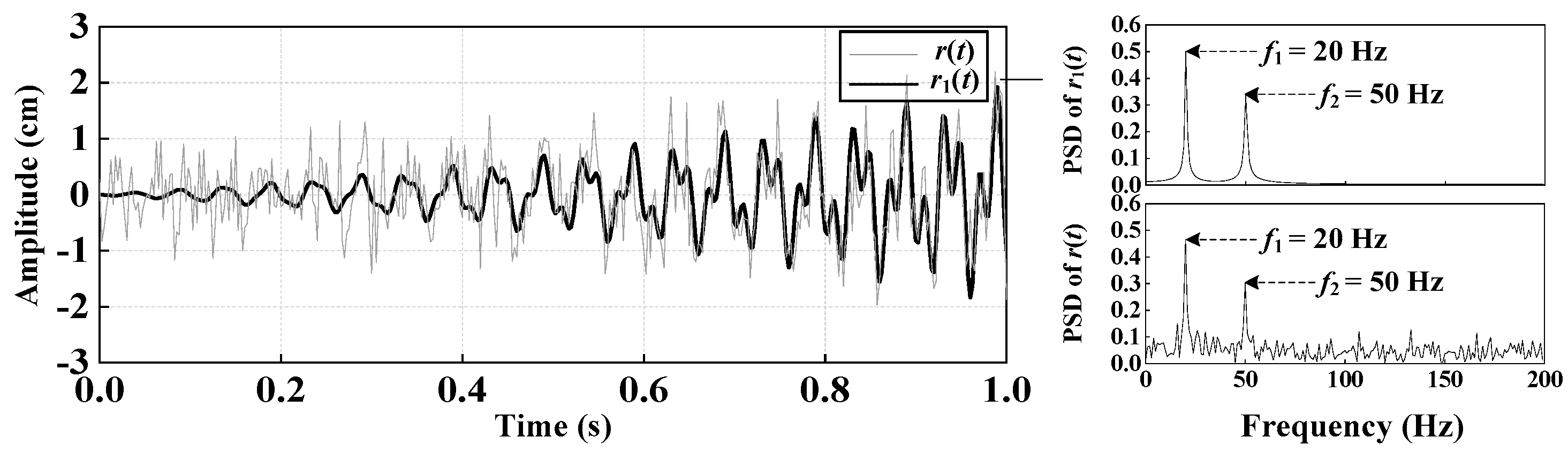
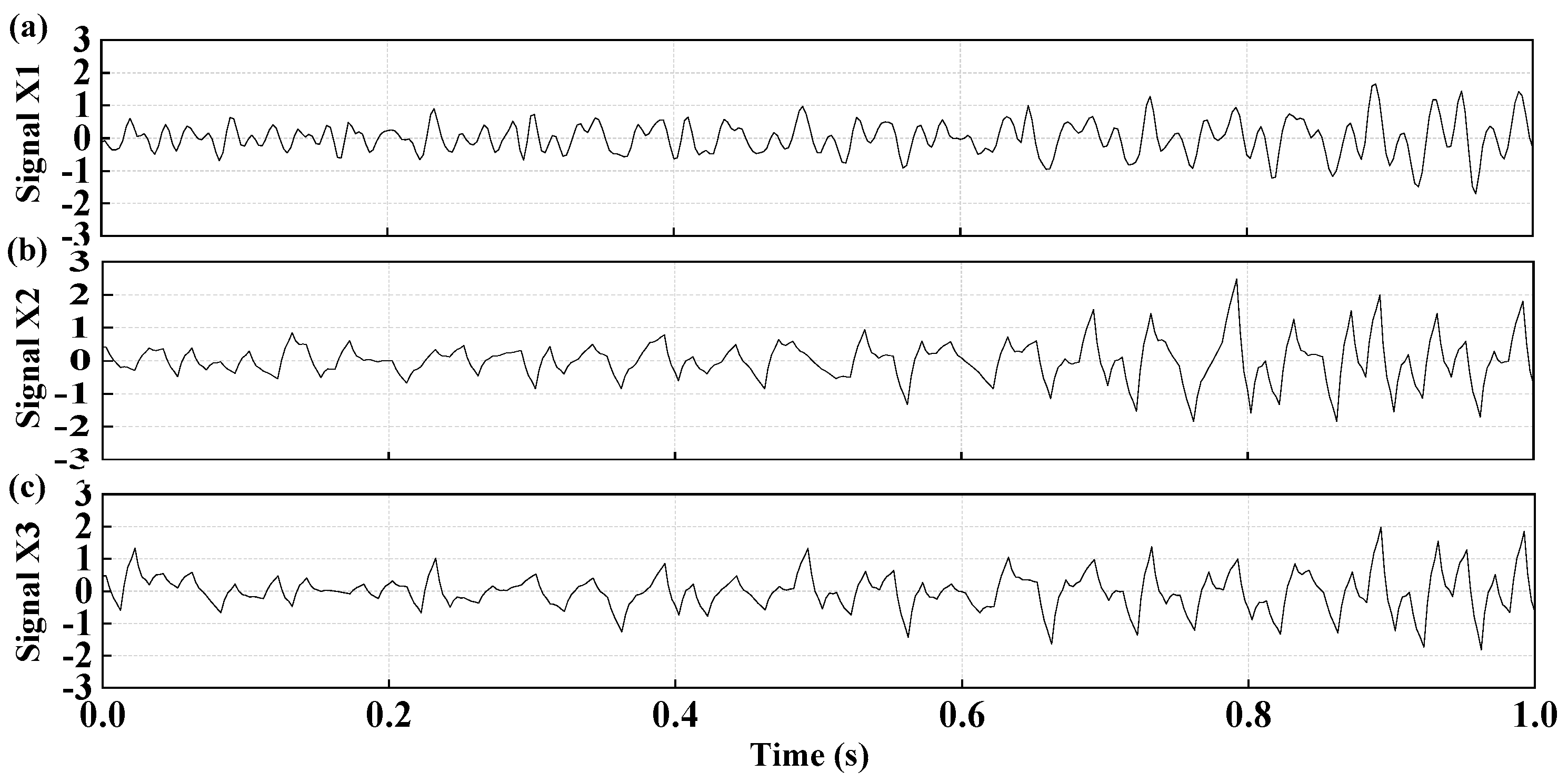
4. Performance Evaluation of the CEEMDAN-WP

In order to evaluate the performance of the CEEMDAN-WP, we consider the nonlinear signal

$$r\left(t\right)=\underset{r_1\left(t\right)}{\underbrace{-t\sin \left(2\pi f_{1}t\right)-t^2\cos \left(2\pi f_{2}t\right)}}+r_2\left(t\right)$$

(19)

where $f_1=20\mathrm{Hz}$, $f_2=50\mathrm{Hz}$, and $r_2\left(t\right)$ are the noise signals with a SNR of 5 dB. The sampling rate is set to 400 Hz and the sampling time is 1 s. Moreover, it is assumed that the unit of signal $r\left(t\right)$ is centimeter (cm). Figure 4 shows the vibration amplitudes of signals $r\left(t\right)$ and $r_1\left(t\right)$, as well as their PSD functions. Following this, the signal $r\left(t\right)$ is processed by employing CEEMDAN, CEEMDAN-WP, and WP, separately.

Based on the CEEMDAN and FFT methods, nine IMF components and their corresponding PSD functions were obtained, as shown in Figure 5. It can be seen that the IMF2–IMF4 components contain the dominate frequency information of the signal. Hence, they were retained, and the other components were removed. This is equivalent to forming a band-pass filter. Figure 6a shows the vibration amplitude of the first-time restructured signal (Signal X1). Following this, a three-level WP technique was applied to denoise the signal X1, and the second-time restructured signal (Signal X2) was obtained, as shown in Figure 6b. Additionally, a single WP technique was employed to denoise the signal $r\left(t\right)$, and the result (Signal X3) is depicted in Figure 6c. In general, SNR and root mean square error (RMSE) play important roles in evaluating the effect of noise reduction. They take the forms

$$\mathrm{SNR}=10{\log }_{10}\left\{\frac{{\displaystyle {\sum }_{i=1}^n{S}_i^2}}{{\displaystyle {\sum }_{i=1}^n{\left(S_i-{S^{\prime }}_i\right)}^2}}\right\}$$

(20)

$$\mathrm{RMSE}=\sqrt{\frac{1}{n}{\displaystyle \sum _{i=1}^n{\left(S_i-{S^{\prime }}_i\right)}^2}}$$

(21)

where $S_i$ and ${S^{\prime }}_i$ represent the real signal and the denoised signal, respectively, and n is the length of the signal. The maximum SNR and minimum RMSE are better with regard to the effect of noise reduction.

Table 1. Statistical results of signal–noise ratio (SNR) and root mean square error (RMSE).

	CEEMDAN	WP	CEEMDAN-WP
SNR	9.7908	9.3499	10.2086
RMSE (cm)	0.3187	0.3258	0.3121

shows the statistical results of SNR and RMSE under the three different denoising methods. In Table 1, it can be seen that the SNR obtained via the CEEMDAN-WP method is higher than that obtained using the other two methods. The RMSE obtained via the CEEMDAN-WP method is lower than that obtained using the other two methods. That is to say, the CEEMDAN-WP outperforms the single CEEMDAN and WP methods. Hence, based on the GNSS-RTK measurement, the vibration signals of a long-span bridge may be denoised by employing the CEEMDAN-WP method.

5. Structural Dynamic Deformation Monitoring of Rainbow Bridge

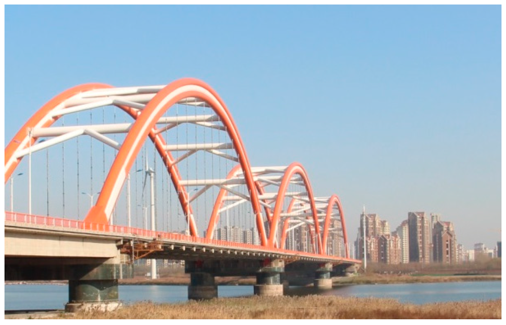
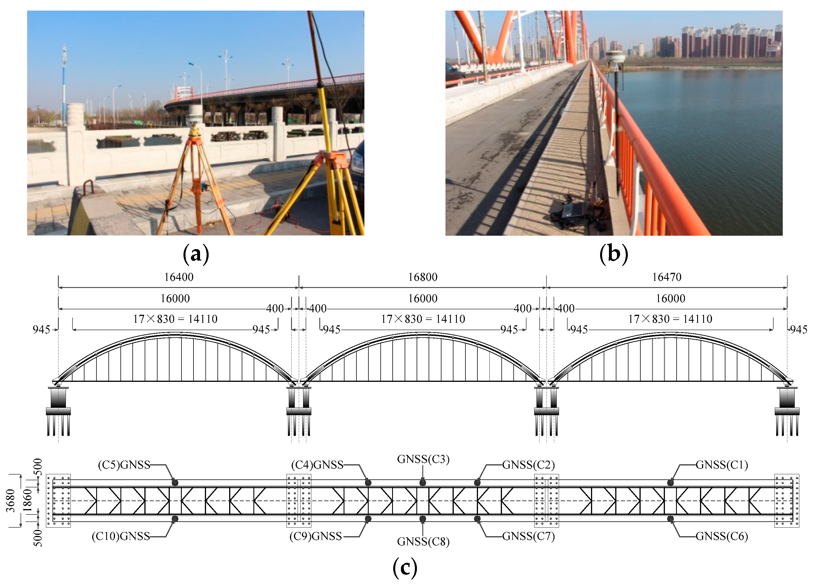
5.1. Bridge Description and Test Plan

We will now consider a long-span concrete-filled steel tubular arch bridge, which is called Rainbow Bridge, as shown in Figure 7. The bridge is located in the east part of Tianjin, China and has a length of 1215.69 m. The main bridge length is 504 m and the width is 29 m. It is a rigid arch system with a simple supported down bearing flexible tie rod, a total of three holes, and a calculation span of 160 m. Its vector height is 32 m and its vector span ratio is 1:5. The arch axis of the bridge adopts catenary with an arch axis coefficient of 1.5. To date, due to the long-term passage of overweight vehicles far exceeding the design load, serious damage has been caused to the safety of Rainbow Bridge. In June 2010, a longitudinal concrete beam of the main bridge cracked, resulting in varying degrees of damage to the two adjacent longitudinal concrete beams. An examining report showed that the bridge contained hidden safety issues. Subsequently, all longitudinal concrete beams were replaced with combined beams. Large trucks are now restricted from using the bridge. Therefore, it is of great importance to study the vibration characteristics of Rainbow Bridge and ensure its safety.

This section introduces a bridge structure monitoring system based on GNSS-RTK sensors. The dynamic deformation of the Rainbow Bridge under ambient excitation, including the influence of vehicular load, was monitored using a 10 Hz sampling frequency. The position of the GNSS-RTK reference station receiver was ~200 m from the Rainbow Bridge. To avoid the influence of ambient excitation on the reference station, the tripod for the fixed reference station receiver was placed on stable ground subject to no traffic interference, as shown in Figure 8a. Ten GNSS-RTK rover stations were employed to monitor the bridge through these vertical vibration response data were collected. The rover stations were symmetrically arranged on both sides of the Rainbow Bridge, as illustrated in Figure 8b. Figure 8c illustrates the schematic locations.

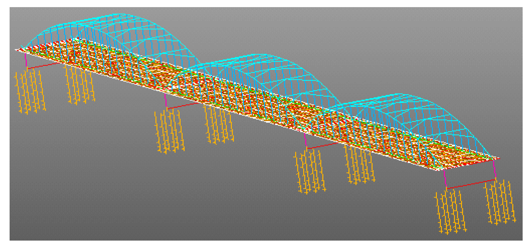
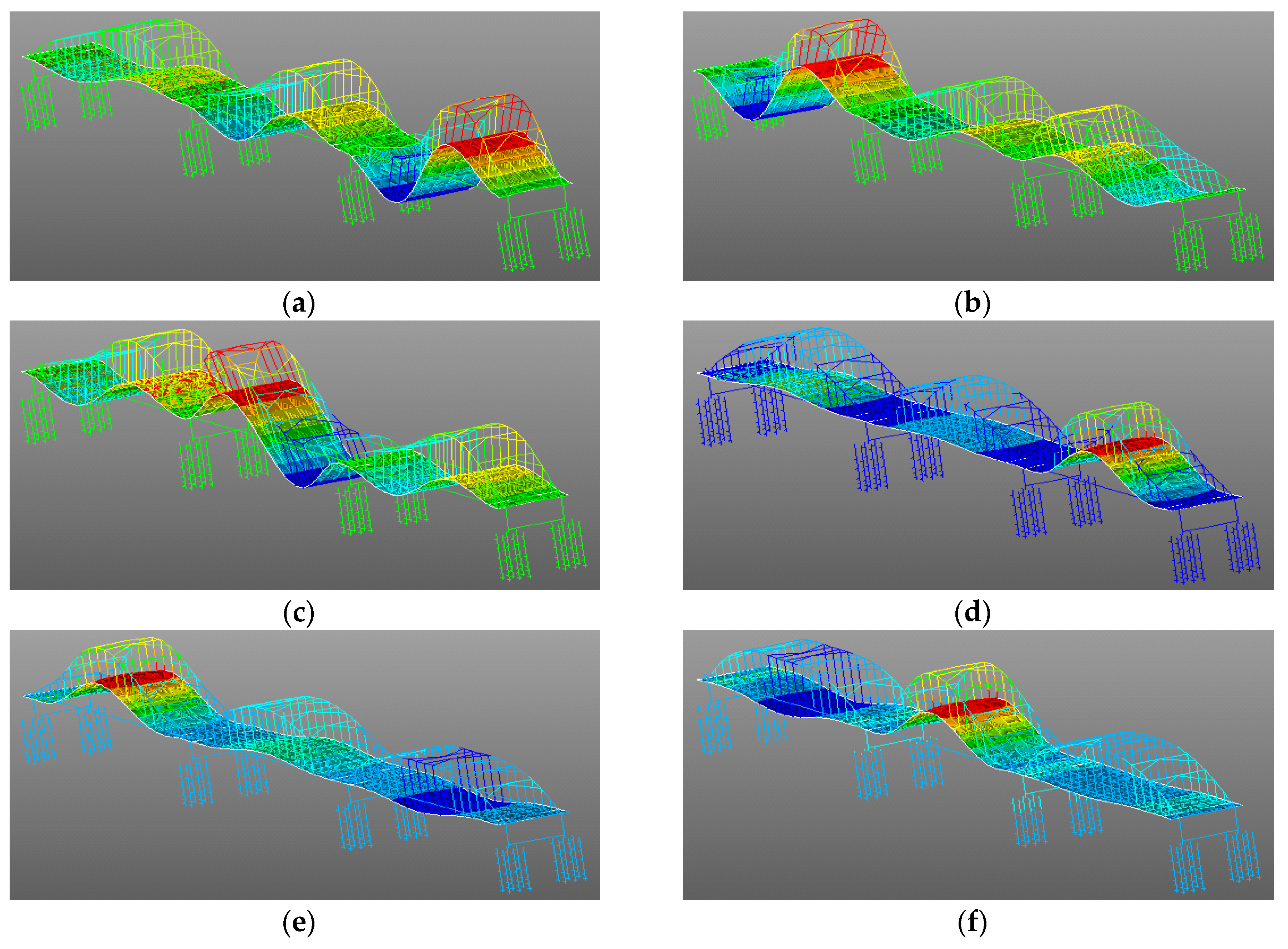
5.2. FEM of the Bridge

Finite element analysis software—ANSYS 14.5—was selected as the tool used to establish FEM of the Rainbow Bridge, and via this software the bridge’s structural dynamic characteristics were evaluated. Figure 9 shows the FEM of Rainbow Bridge. There are 1765 nodes and 2727 elements in this FEM model. The steel pipe, wind brace, crossbeam, stringer, and pier are represented by BEAM44. When considering the plasticity of materials, the BEAM188 element was elected. The link10 and shell63 elements were used to simulate the tie bars and the deck of the bridge, respectively. There were six degrees of freedom (DOF) for every node, including the translational DOF along the x, y, and z directions and the rotational DOF around the x, y, and z axes, individually.

Table 2. Parameters for the structural finite element model (FEM).

	Steel Tube and Wind Brace	Concrete Inside the Steel Tube	Crossbeam and Stringer	Tie Bar	Bridge Deck	Pier Column
Elasticity modulus (Pa)	2.1 × 1011	3.5 × 1010	3.0 × 1010	2.1 × 1011	2.85 × 1010	3.3 × 1010
Density (kg/m3)	7800	2600	2600	7800	2500	2600
Poisson coefficient	0.3	0.1667	0.1667	0.3	0.1667	0.1667

illustrates the relevant parameters for FEM. Finally, we obtained the first six natural frequencies (i.e., 0.1632 Hz, 0.6787 Hz, 0.8171 Hz, 0.8254 Hz, 0.9225 Hz, and 0.9945 Hz) of the structure. The structural mode shapes of the first six orders are shown in Figure 10a–f, which may offer some references for the field monitoring.

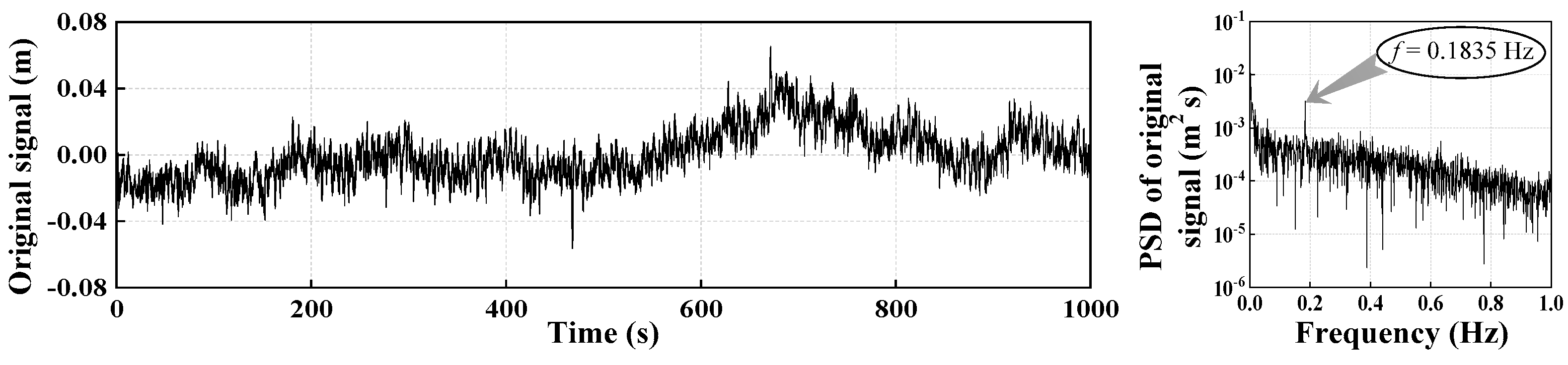
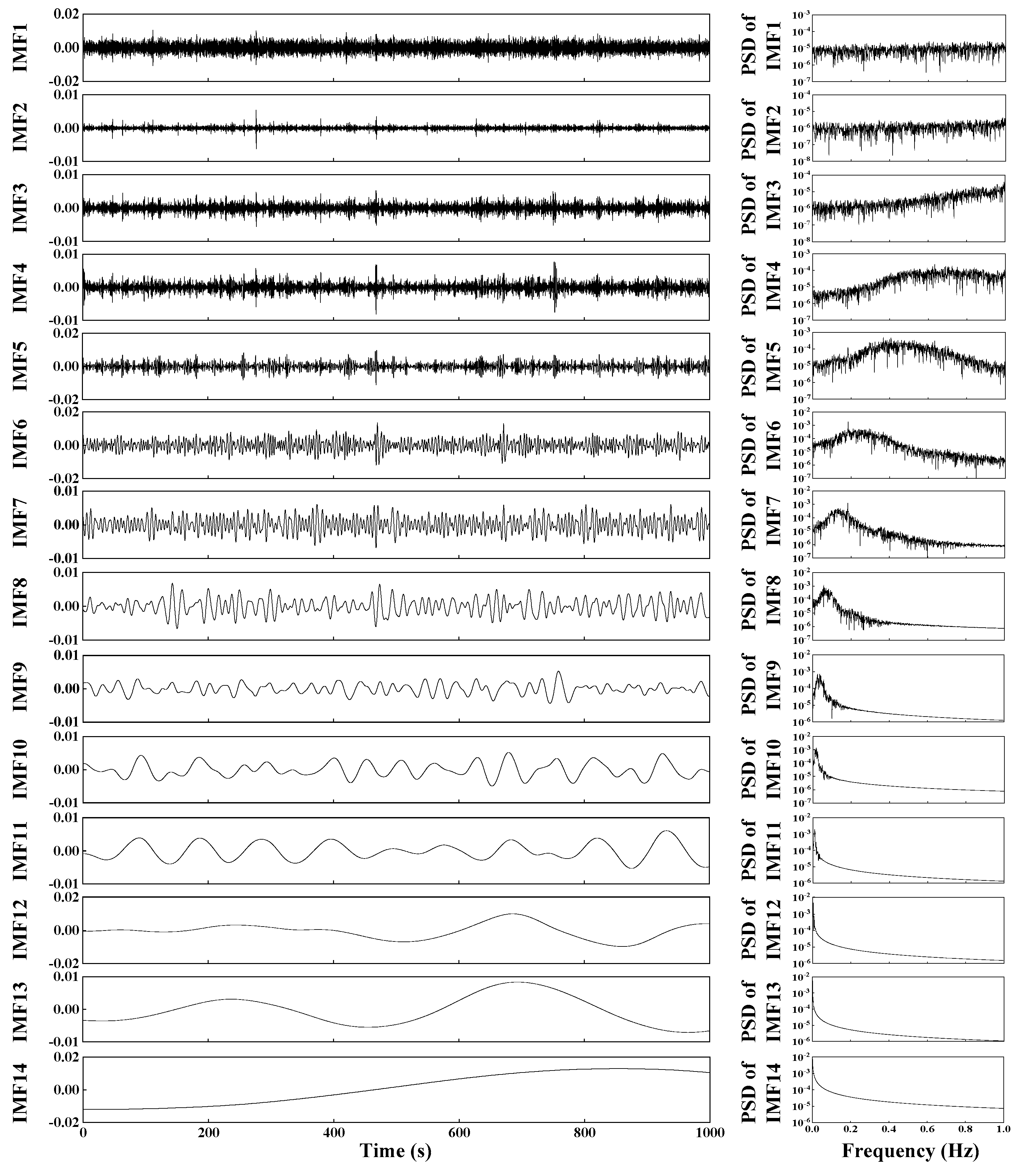
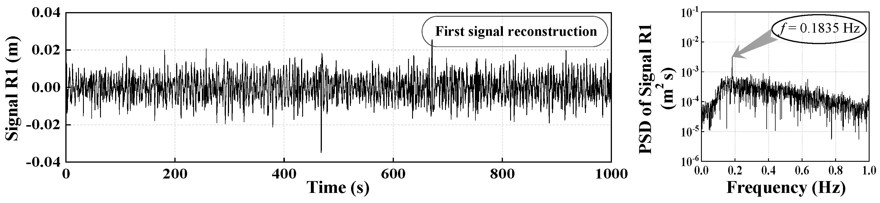
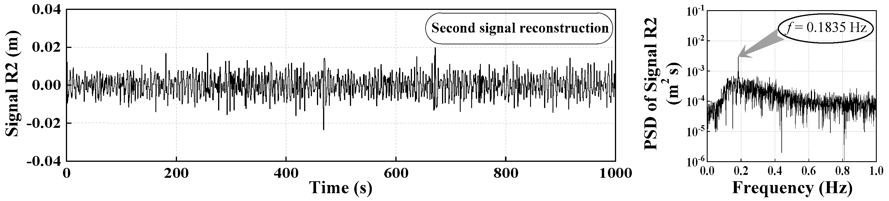
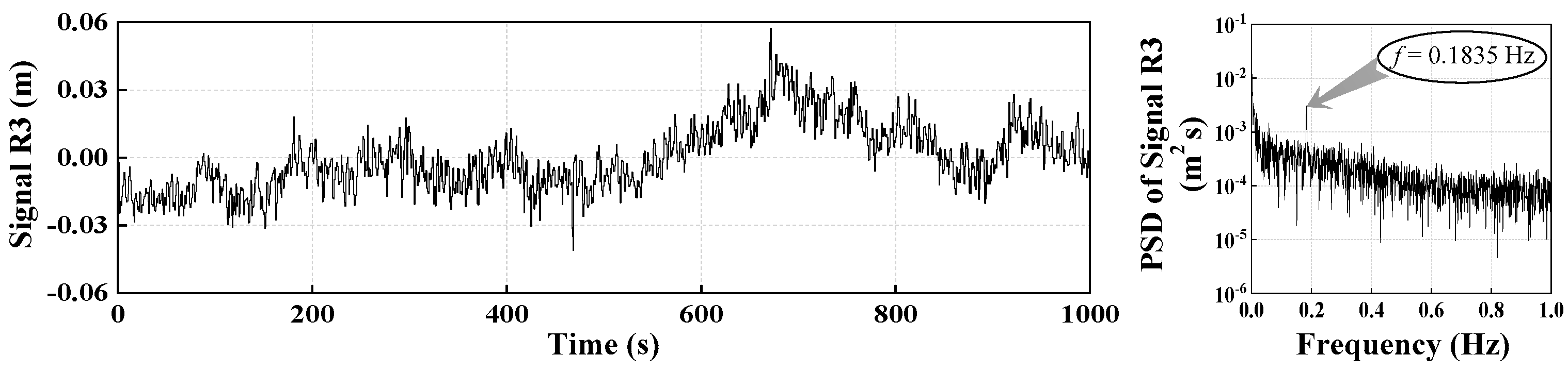
5.3. Vibration Signal Analysis

As depicted in Nyquist sampling theory, when the sampling frequency is greater than twice the highest frequency of the signal, the digital signal completely retains the information of the original signal; thus, the sampling signal can be reconstructed as the initial continuous form without the loss of information. According to the numerical simulation results in the previous section, the first order natural frequency (i.e., 0.1632 Hz) is much less than 10 Hz. Therefore, this sampling frequency meets the theoretical requirements.

Dynamic deformation monitoring was conducted for 10 consecutive hours from 9:00 a.m. to 7:00 p.m. on 24 February 2017. The collected data and its PSD function at the monitored point C3 are shown in Figure 11. The amplitude of the vertical vibration displacement is within −0.0564~0.0652 m. FFT was employed to identify the structural natural frequency. There is an obvious peak corresponding to the structurally dominant frequency (i.e., 0.1835 Hz). Compared with the result of the numerical analysis, the identified modal parameter of the bridge using the FFT method is larger. We obtained noise distribution characteristics according to the stability experiment. The proposed combined denoising method was employed to deal with both low-frequency and high-frequency noise. At first, the original signal was decomposed by the CEEMDAN method and 14 IMFs were obtained. Figure 12 illustrates the 14 IMFs and their corresponding PSD functions, from which we can conclude that the components containing the structural natural frequency is mainly distributed within IMF6–IMF8. IMF1–IMF3 and IMF11–IMF14 components should be removed because they contain a lot of high-frequency and low-frequency noise, respectively. This operation is the equivalent of denoising with a band-pass filter. IMF6–IMF8 components were reconstructed as Signal R1. Signal R1 and its PSD function are shown in Figure 13. It is obvious that the amplitude of the displacement (i.e., −0.0349–0.0257 m) was significantly reduced following reconstruction. In addition low-frequency noise was effectively eliminated. Subsequently, the three-layer WP technique was used to deal with Signal R1, and thus Signal R2 was derived. As shown in Figure 14, the amplitude of displacement (i.e., −0.0235–0.0198 m) was further reduced. Moreover, a single WP technique was adopted to denoise the original signal from Figure 11, with the result (i.e., Signal R3) indicated in Figure 15. Meanwhile, the RMS of the original signal, Signal R3, Signal R1, and Signal R2 were obtained, being 0.0153 m, 0.0147 m, 0.0064 m, and 0.0056 m, respectively. In view of the above discussion, it may be concluded that the combined method used in this paper is more effective than the individual application of CEEMDAN or WP.

In general, the damping ratio selected for design is estimated empirically. Therefore, it is of great importance to use the RDT method to obtain a damping ratio from the field measured data. In some research, the value of subsample N has been in the range of 400 to 2000 [42]. In this paper, the value of N is defined as 1500, and different values of the time interval were chosen as $\tau =100\mathrm{s}$, $\tau =150\mathrm{s}$, and $\tau =200\mathrm{s}$. Figure 16 illustrates the computed results of the RDS, and the structural damping ratios corresponding to different $\tau$ values can be obtained via Equation (23) (i.e., $\tau =100\mathrm{s}\xi =1.77\%$; $\tau =150\mathrm{s}\xi =1.70\%$; and $\tau =200\mathrm{s}\xi =1.73\%$). The results indicate that the damping ratio is close to 1.73%. The natural frequency and its corresponding damping ratio have been identified successfully.

6. Conclusions

This article has focused on the dynamic deformation monitoring of Tianjin Rainbow Bridge using GNSS-RTK and the corresponding modal parameters, which were analyzed via the employment of FFT and RDT. With a focus on the existence of noise in the signal, we proposed a combined denoising method, called CEEMDAN-WP. An FEM of the bridge was established in order to provide a reference with which to compare the field measurement results. Through an analysis of our field measurement and finite element simulation results, we were able to draw the following conclusions. (1) The GNSS-RTK technique can be used to monitor the dynamic response of long-span bridges under ambient excitation. The sampling frequency and noise intensity of the GNSS-RTK receivers essentially meet the requirements of field measurement. (2) The proposed CEEMDAN-WP method is an efficient means with which to eliminate both low-frequency and high-frequency noise without distortion. (3) Through FFT and RDT analysis, a first natural frequency of Tianjin Rainbow Bridge of 0.1835 Hz and a corresponding damping ratio of 1.73% were obtained. (4) The identified natural frequency obtained from the processed signal was observed to be slightly greater than the FEM value and the difference between them was about 11%. This may have been caused by bridge damage or the inadequate accuracy of the finite element model.

References

1. Piombo, B.A.D.; Fasana, A.; Marchesiello, S.; Ruzzene, M. Modelling and identification of the dynamic response of a supported bridge. Mech. Syst. Signal Process. 2000, 14, 75–89. [Google Scholar] [CrossRef]
2. Fenerci, A.; Øiseth, O.; Rønnquist, A. Long-term monitoring of wind field characteristics and dynamic response of a long-span suspension bridge in complex terrain. Eng. Struct. 2017, 147, 269–284. [Google Scholar] [CrossRef]
3. Masri, S.F.; Sheng, L.H.; Caffrey, J.P.; Nigbor, R.L.; Wahbeh, M.; Abdel-Ghaffar, A.M. Application of a web-enabled real-time structural health monitoring system for civil infrastructure systems. Smart Mater. Struct. 2004, 13, 1269–1283. [Google Scholar] [CrossRef]
4. Lee, J.J.; Shinozuka, M. A vision-based system for remote sensing of bridge displacement. NDT E Int. 2006, 39, 425–431. [Google Scholar] [CrossRef]
5. Yi, T.H.; Li, H.N.; Song, G.B.; Guo, Q. Detection of Shifts in GPS Measurements for a Long-Span Bridge Using CUSUM Chart. Int. J. Struct. Stab. Dyn. 2016, 16, 1640024. [Google Scholar] [CrossRef]
6. Górski, P. Investigation of dynamic characteristics of tall industrial chimney based on GPS measurements using Random Decrement Method. Eng. Struct. 2015, 83, 30–49. [Google Scholar] [CrossRef]
7. Kalkan, Y.; Potts, L.V.; Bilgi, S. Assessment of vertical deformation of the atatürk dam using geodetic observations. J. Surv. Eng. 2016, 142, 04015011. [Google Scholar] [CrossRef]
8. Xiong, C.B.; Niu, Y.B.; Li, Z. An investigation of the dynamic characteristics of super high-rise buildings using real-time kinematic–global navigation satellite system technology. Adv. Struct. Eng. 2018, 21, 783–792. [Google Scholar] [CrossRef]
9. Niu, Y.B.; Xiong, C.B. Analysis of the dynamic characteristics of a suspension bridge based on RTK-GNSS measurement combining EEMD and a wavelet packet technique. Meas. Sci. Technol. 2018, 29, 085103. [Google Scholar] [CrossRef] [Green Version]
10. Xiong, C.B.; Niu, Y.B. Investigation of the dynamic behavior of a super high-rise structure using RTK-GNSS technique. KSCE J. Civ. Eng. 2019, 23, 654–665. [Google Scholar] [CrossRef]
11. Ince, C.D.; Sahin, M. Real-time deformation monitoring with GPS and Kalman Filter. J. Earth Planets Space 2000, 52, 837–840. [Google Scholar] [CrossRef] [Green Version]
12. Li, X.; Zhang, X.; Ren, X.; Fritsche, M.; Wickert, J.; Schuh, H. Precise positioning with current multi-constellation Global Navigation Satellite Systems: GPS, GLONASS, Galileo and BeiDou. Sci. Rep. 2015, 5, 8328–8341. [Google Scholar] [CrossRef] [PubMed]
13. Huang, N.E.; Shen, Z.; Long, S.R.; Wu, M.C.; Shih, H.H.; Zheng, Q.; Yen, N.C.; Tung, C.C.; Liu, H.H. The empirical mode decomposition and the Hilbert spectrum for nonlinear and non-stationary time series analysis. Proc. R. Soc. Lond. Ser. A Math. Phys. Eng. Sci. 1998, 454, 903–995. [Google Scholar] [CrossRef]
14. Wu, Z.; Huang, N.E. Ensemble empirical mode decomposition: A noise-assisted data analysis method. Adv. Adapt. Data Anal. 2009, 1, 1–41. [Google Scholar] [CrossRef]
15. Yeh, J.R.; Shieh, J.S.; Huang, N.E. Complementary ensemble empirical mode decomposition: A novel noise enhanced data analysis method. Adv. Adapt. Data Anal. 2010, 2, 135–156. [Google Scholar] [CrossRef]
16. Torres, M.E.; Colominas, M.A.; Schlotthauer, G.; Flandrin, P. A complete ensemble empirical mode decomposition with adaptive noise. In Proceedings of the 2011 IEEE International Conference on Acoustics, Speech and Signal (ICASSP), Prague, Czech Republic, 22–27 May 2011; pp. 4144–4147. [Google Scholar]
17. Kurt, M.; Eriten, M.; McFarland, D.M.; Bergman, L.A.; Vakakis, A.F. Strongly nonlinear beats in the dynamics of an elastic system with a strong local stiffness nonlinearity: Analysis and identification. J. Sound Vib. 2014, 333, 2054–2072. [Google Scholar] [CrossRef]
18. Kurt, M.; Chen, H.; Lee, Y.S.; McFarland, D.M.; Bergman, L.A.; Vakakis, A.F. Nonlinear system identification of the dynamics of a vibro-impact beam: Numerical results. Arch. Appl. Mech. 2012, 82, 1461–1479. [Google Scholar] [CrossRef]
19. Moore, K.J.; Kurt, M.; Eriten, M.; McFarland, D.M.; Bergman, L.A.; Vakakis, A.F. Wavelet-bounded empirical mode decomposition for vibro-impact analysis. Nonlinear Dyn. 2018, 93, 1559–1577. [Google Scholar] [CrossRef]
20. Moore, K.J.; Kurt, M.; Eriten, M.; McFarland, D.M.; Bergman, L.A.; Vakakis, A.F. Wavelet-bounded empirical mode decomposition for measured time series analysis. Mech. Syst. Signal Process. 2018, 99, 14–29. [Google Scholar] [CrossRef]
21. Kijecwski, T.; Kareem, A. Wavelet transforms for systems identification in civil engineering. Comput.-Aided Civ. Inf. 2003, 18, 339–355. [Google Scholar] [CrossRef]
22. Giaouris, D.; Fincth, J.W. De-noising using wavelets on electric drive applications. Electr. Power Syst. Res. 2008, 78, 559–565. [Google Scholar] [CrossRef]
23. Liu, F.; Ruan, X.E. Wavelet-based diffusion approaches for signal de-noising. Signal Process 2007, 87, 1138–1146. [Google Scholar] [CrossRef]
24. Perez-Ramirez, C.A.; Jaen-Cuellar, A.Y.; Valtierra-Rodriguez, M.; Dominguez-Gonzalez, A.; Osornio-Rios, R.A.; Romero-Troncoso, R.J.; Amezquita-Sanchez, J.P. A two-step strategy for system identification of civil structures for structural health monitoring using wavelet transform and genetic algorithms. Appl. Sci. 2017, 7, 111. [Google Scholar] [CrossRef]
25. Zhang, X.; Song, K.; Li, C.G.; Yang, L.X. A novel approach for the estimation of doubly spread acoustic channels based on wavelet transform. Appl. Sci. 2018, 8, 38. [Google Scholar] [CrossRef]
26. Farzad, H.; Wasim, O.; Mohamed, G. Roller bearing acoustic signature extraction by wavelet packet transform, applications in fault detection and size estimation. Appl. Acoust. 2016, 104, 101–118. [Google Scholar]
27. Lau, L. Wavelet packets based denoising method for measurement domain repeat-time multipath filtering in GPS static high-precision positioning. GPS Solut. 2017, 21, 461–474. [Google Scholar] [CrossRef]
28. Ding, Y.L.; Li, A.Q.; Deng, Y. Structural Damage Warning of a Long-Span Cable-Stayed Bridge Using Novelty Detection Technique Based on Wavelet Packet Analysis. Adv. Struct. Eng. 2010, 13, 291–298. [Google Scholar] [CrossRef]
29. García-Plaza, E.; Núñez, P.J. Application of the wavelet packet transform to vibration signals for surface roughness monitoring in CNC turning operations. Mech. Syst. Signal Process. 2018, 98, 902–919. [Google Scholar] [CrossRef]
30. Ding, Y.L.; Li, A.Q. Structural health monitoring of long-span suspension bridges using wavelet packet analysis. Earthq. Eng. Eng. Vib. 2007, 6, 289–294. [Google Scholar] [CrossRef]
31. Sirca, G.F.; Adeli, H. System identification in structural engineering. Sci. Iran. 2012, 19, 1355–1364. [Google Scholar] [CrossRef] [Green Version]
32. Wang, X.; Wu, Z.S. Modal damping evaluation of hybrid FRP cable with smart dampers for long-span cable-stayed bridges. Compos. Struct. 2011, 93, 1231–1238. [Google Scholar] [CrossRef]
33. Tamura, Y.; Yoshida, A.; Zhang, L. Damping in buildings and estimation techniques. In Proceedings of the 6th Asia-Pacific Conference on Wind Engineering, Seoul, Korea, 12–14 September 2005; pp. 193–214. [Google Scholar]
34. Asmussen, J.C.; Ibrahim, R.; Brincker, R. Random decrement: Identification of structures subjected to ambient excitation. In Proceedings of the 16th International Modal Analysis Conference, Santa Barbara, CA, USA, 2–5 February 1998; pp. 914–921. [Google Scholar]
35. Lin, C.S.; Chiang, D.Y. Modal identification from nonstationary ambient vibration data using random decrement algorithm. Comput. Struct. 2013, 119, 104–114. [Google Scholar] [CrossRef]
36. Ibrahim, S.R. Random decrement technique for modal identification of structures. J. Spacecr. Rocket. 2012, 14, 696. [Google Scholar] [CrossRef]
37. Lin, C.S.; Chiang, D.Y. A modified random decrement technique for modal identification from nonstationary ambient response data only. J. Mech. Sci. Technol. 2012, 26, 1687–1696. [Google Scholar] [CrossRef]
38. Kim, Y.; Park, S.G. Wet damping estimation of the scaled segmented hull model using the random decrement technique. Ocean Eng. 2014, 75, 71–80. [Google Scholar] [CrossRef]
39. Modak, S.V.; Rawal, C.; Kundra, T.K. Harmonics elimination algorithm for operational modal analysis using random decrement technique. Mech. Syst. Signal Process. 2010, 24, 922–944. [Google Scholar] [CrossRef]
40. Vandiver, J.K.; Dunwoody, A.B.; Campbell, R.B.; Cook, M.F. A mathematical basis for the random decrement vibration signature analysis technique. ASME J. Mech. Des. 1982, 104, 307–313. [Google Scholar] [CrossRef]
41. Ku, C.J.; Cermak, J.E.; Chou, L.S. Random decrement-based method for modal parameter identification of a dynamic system using acceleration responses. J. Wind Eng. Ind. Aerodyn. 2007, 95, 389–410. [Google Scholar] [CrossRef]
42. Yang, J.C.S.; Dagalakis, N.G.; Everstine, G.C.; Wang, Y.F. Measurement of structural damping using the random decrement technique. Shock Vib. Bull. 1983, 53, 63–71. [Google Scholar]
Figure 1. Schematic figure for stability experiment.
Applsci 09 01301 g001
Figure 2. The vertical displacement and its corresponding power spectral density (PSD) value.
Applsci 09 01301 g002
Figure 3. Flow chart of the combined signal denoising and identifying process.
Applsci 09 01301 g003
Figure 4. The amplitudes of r ( t ) and r 1 ( t ) along with their PSD functions.
Applsci 09 01301 g004
Figure 5. The intrinsic mode function (IMF) components of signal r ( t ) and the corresponding PSD functions.
Applsci 09 01301 g005
Figure 6. The amplitudes of denoising signals: (a) signal X1; (b) signal X2; and (c) signal X3.
Applsci 09 01301 g006
Figure 7. Panoramic schematic of Rainbow Bridge.
Applsci 09 01301 g007
Figure 8. (a) The arrangement of the GNSS-RTK reference station; (b) the arrangement of GNSS-RTK rover stations; and (c) the schematic locations of the GNSS-RTK rover stations.
Applsci 09 01301 g008
Figure 9. The FEM of Rainbow Bridge.
Applsci 09 01301 g009
Figure 10. (a) The first order of the mode shape, (b) the second order of the mode shape, (c) the third order of the mode shape, (d) the fourth order of the mode shape, (e) the fifth order of the mode shape, and (f) the sixth order of the mode shape.
Applsci 09 01301 g010
Figure 11. Original signal of Point C3 and its PSD function.
Applsci 09 01301 g011
Figure 12. The IMFs of the original signal and their corresponding PSD functions.
Applsci 09 01301 g012
Figure 13. Signal R1 and its PSD function.
Applsci 09 01301 g013
Figure 14. Signal R2 and its PSD function.
Applsci 09 01301 g014
Figure 15. Signal R3 and its PSD function.
Applsci 09 01301 g015
Figure 16. The RDS of Signal R2 for different values of τ .
Applsci 09 01301 g016