Efficient Control of a Non-Linear System Using a Modified Sliding Mode Control


Abstract
1. Introduction
2. Control Design
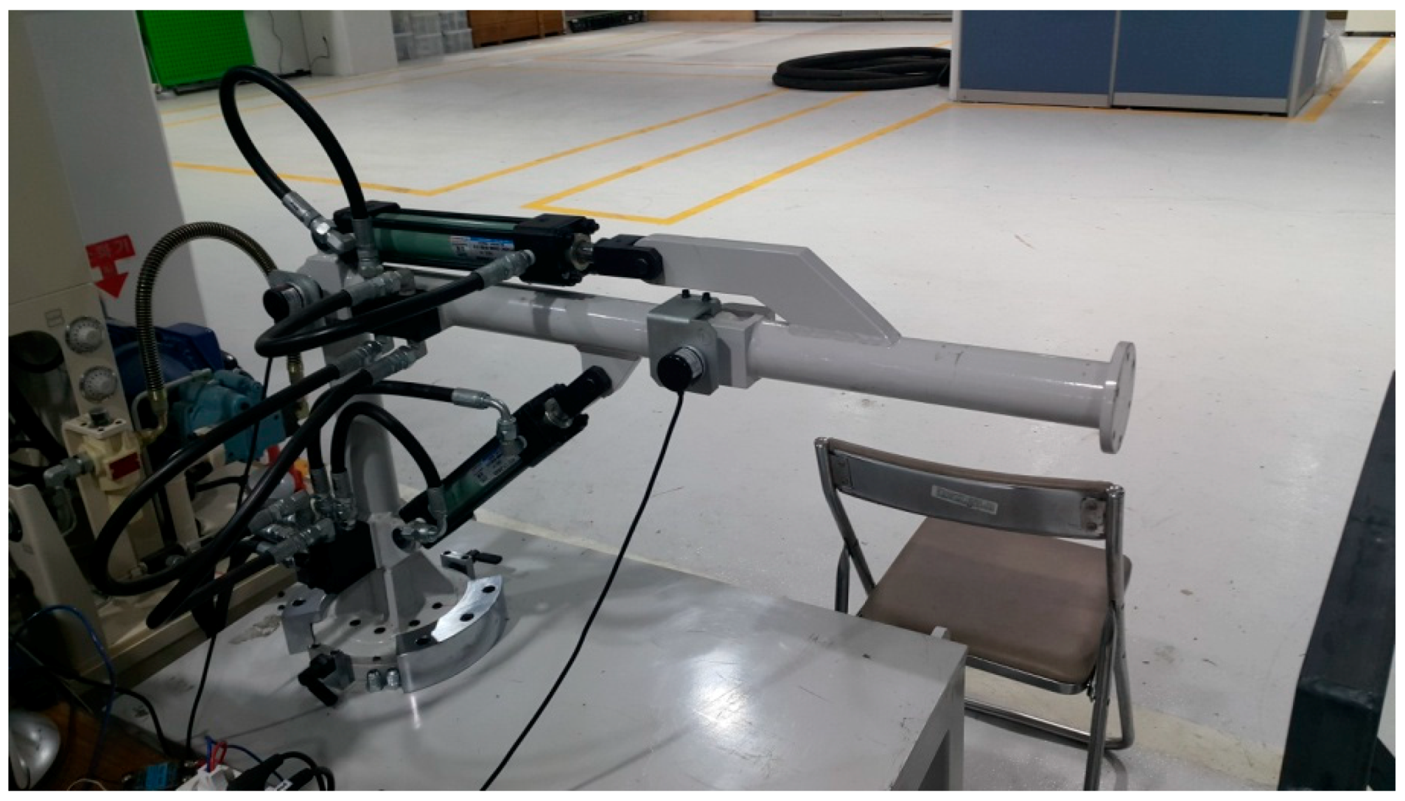
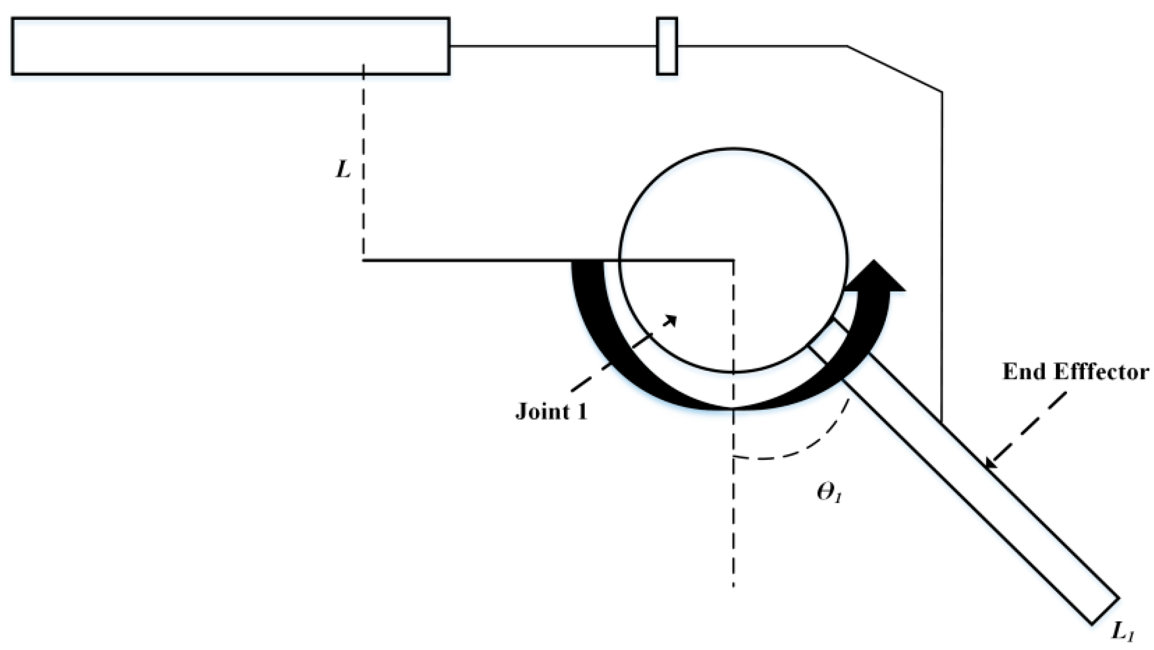
2.1. Dynamics of aHydraulic System
2.2. Sliding Mode Control with Sliding Perturbation Observer (SMCSPO)
2.2.1. Sliding Perturbation Observer (SPO)
2.2.2. Integration of SMC and SPO (SMCSPO)
2.3. PD Sliding Mode Control (PDSMC)
2.3.1. Proposed Scheme Characteristics
2.3.2. Integration of PDSMC and SPO (PDSMCSPO)
2.3.3. Design Procedure
2.3.4. Proposed Scheme Characteristics
3. Simulation and Experimental Results
3.1. Simulation Results of SMC and PDSMC
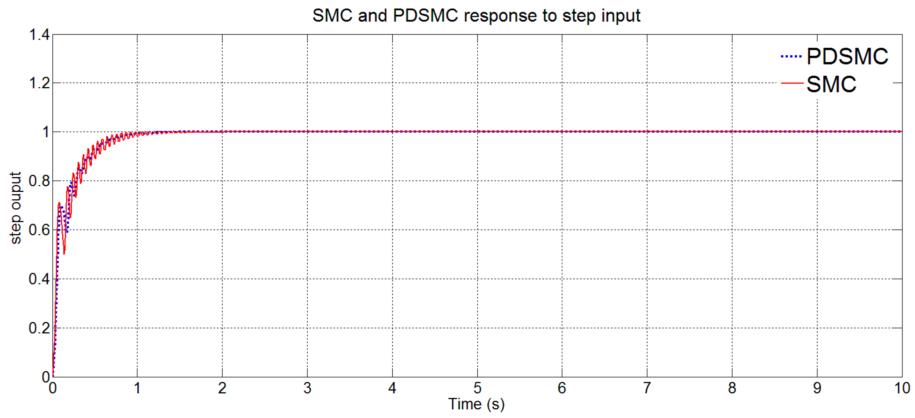
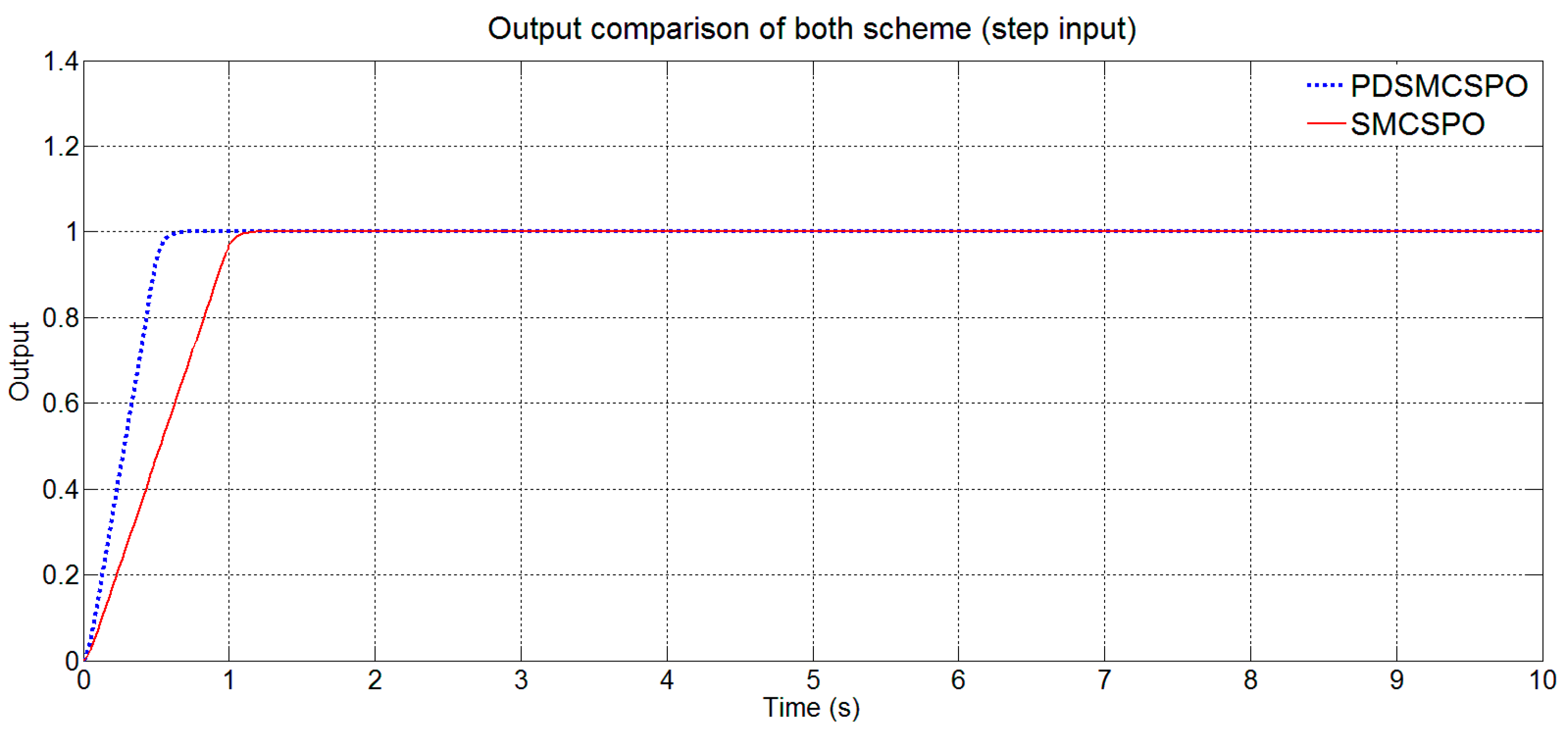
3.1.1. Step Output
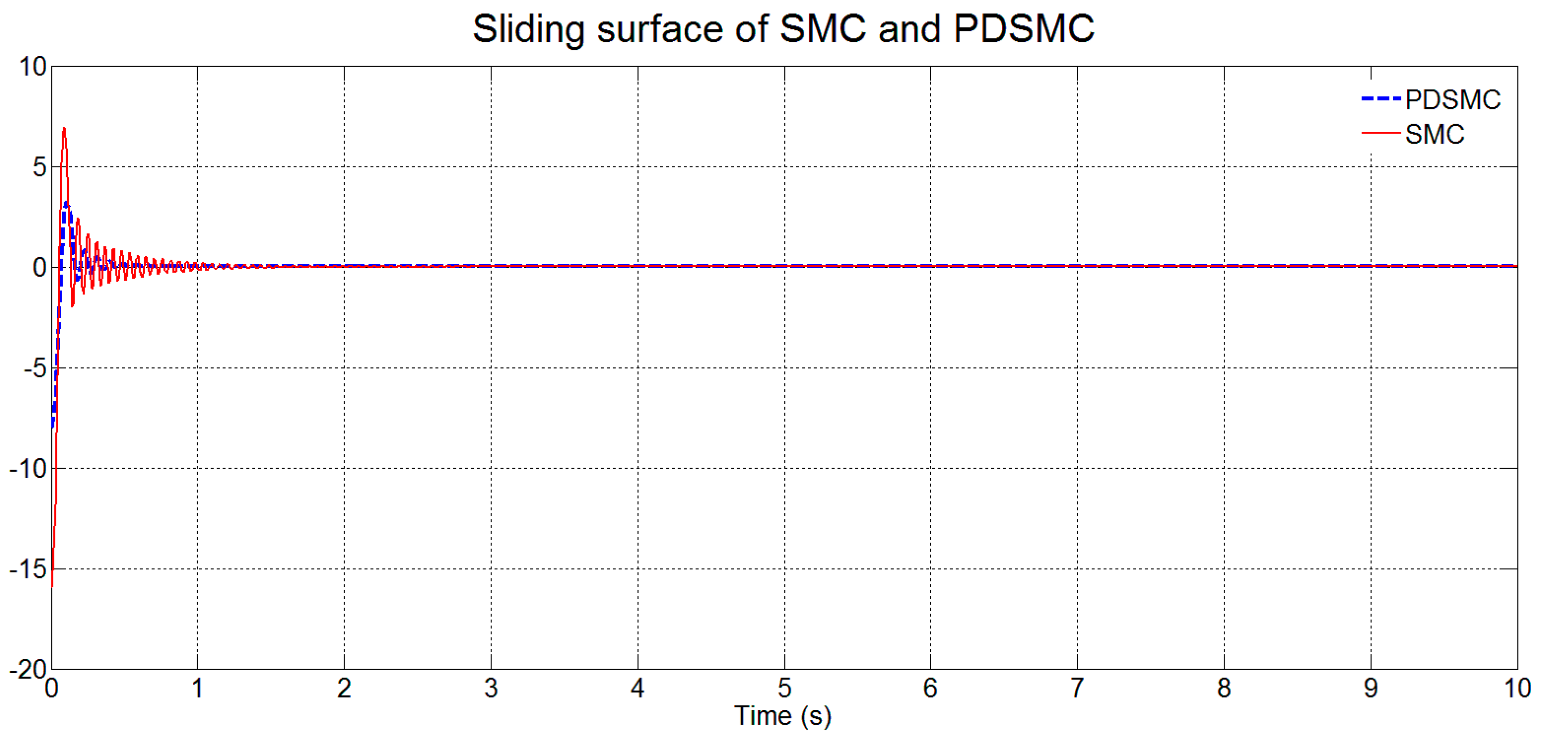
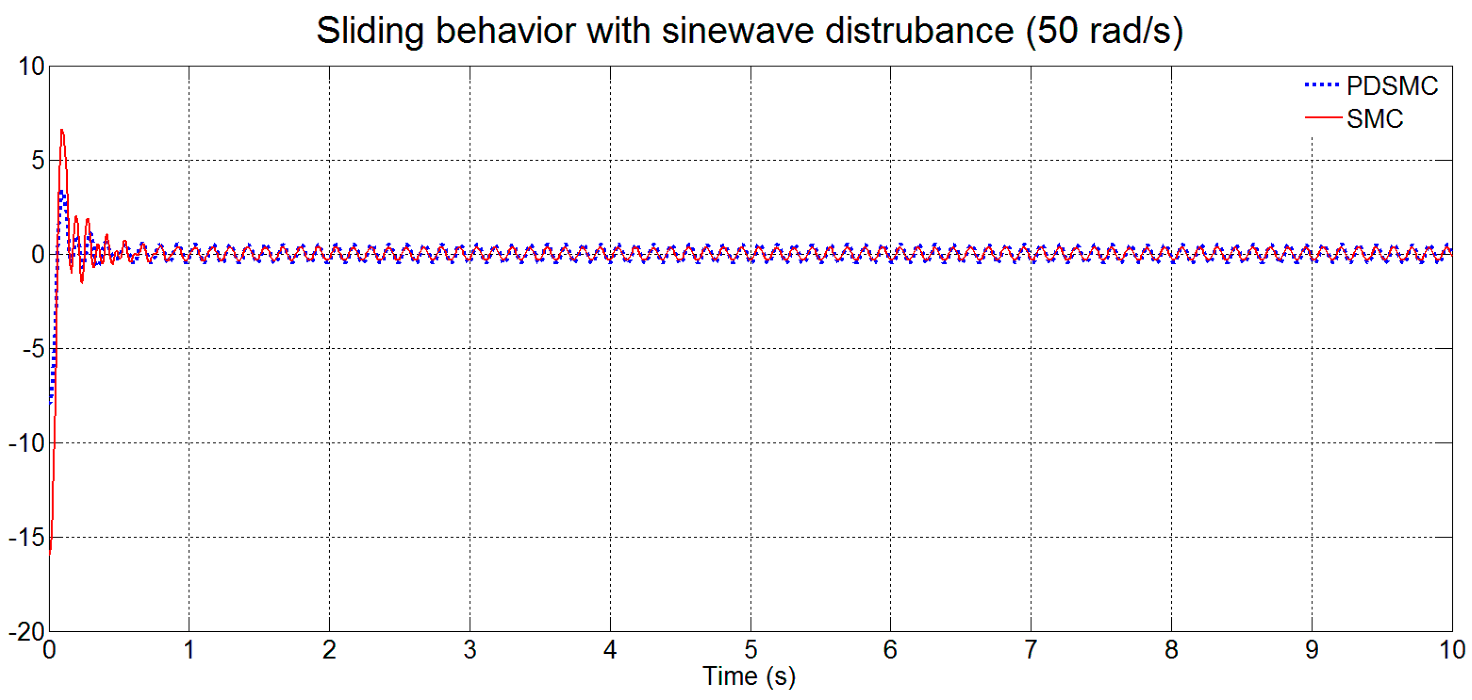
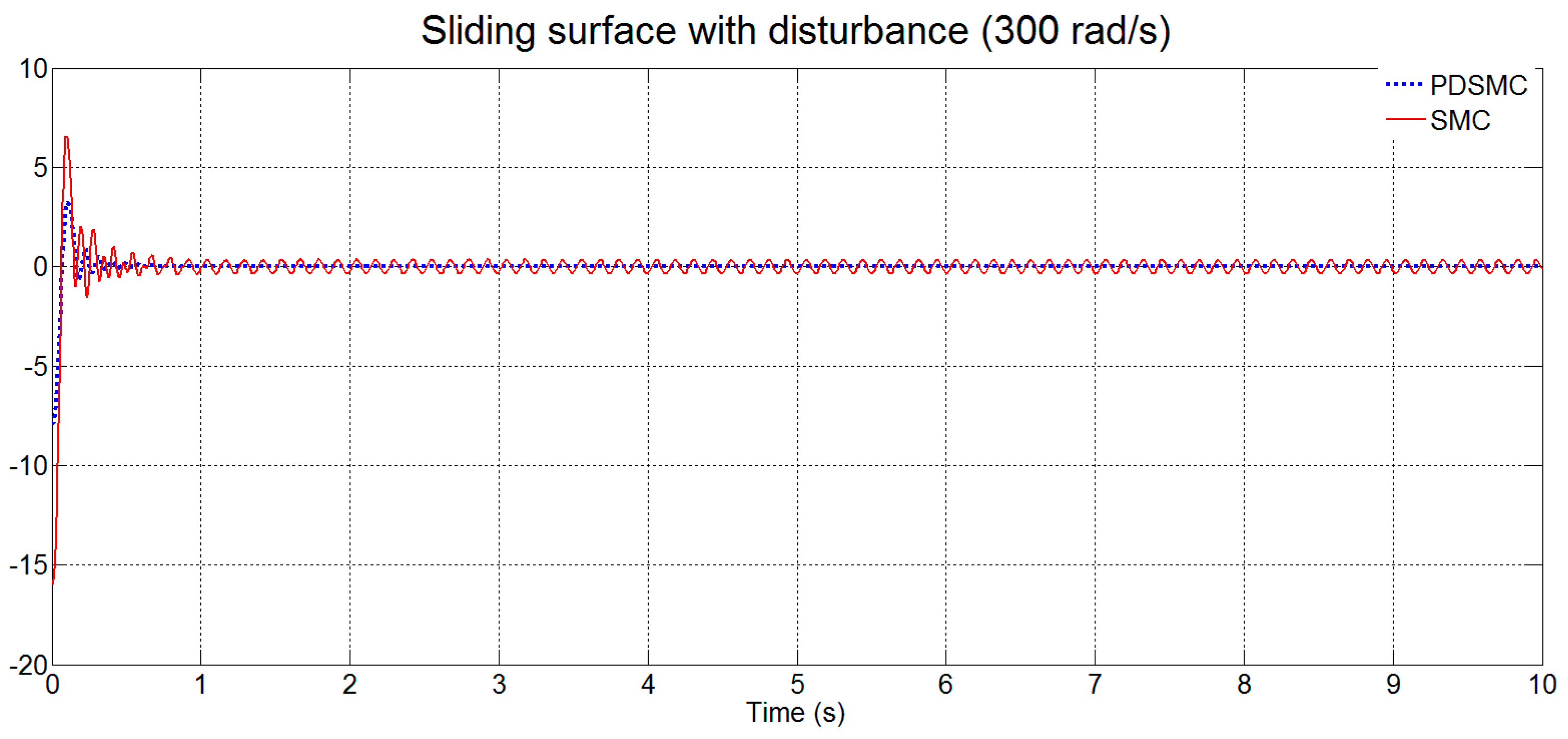
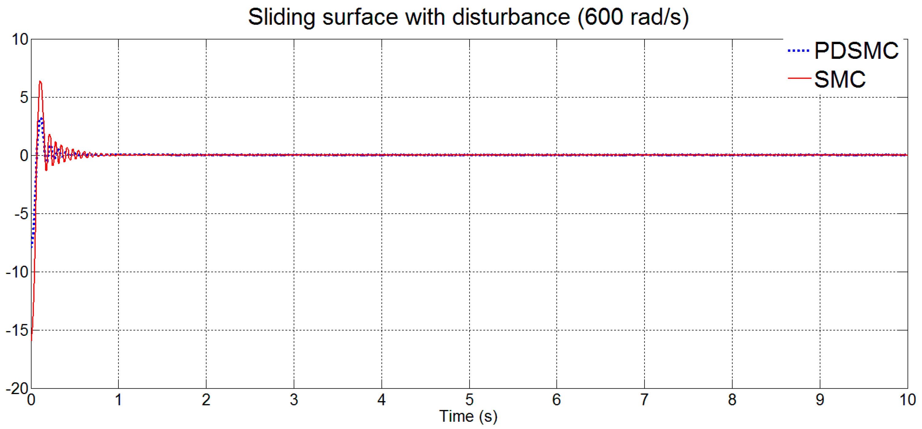
3.1.2. Sliding Surface Response
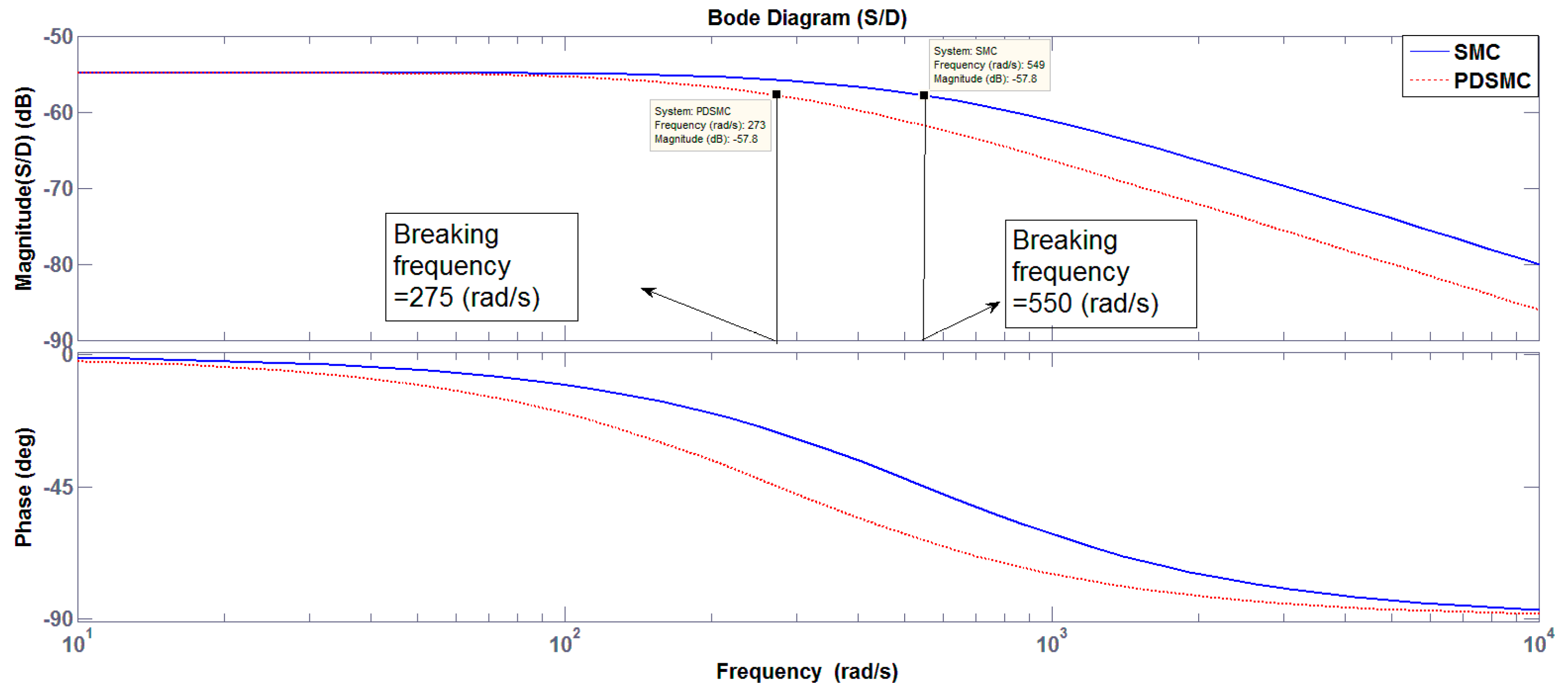
3.1.3. Low Pass Filter Characteristics
Case 1
Case 2
Case 3
3.2. Simulation Results of SMCSPO and PDSMCSPO
3.2.1. SMCSPO
3.2.2. PDSMCSPO
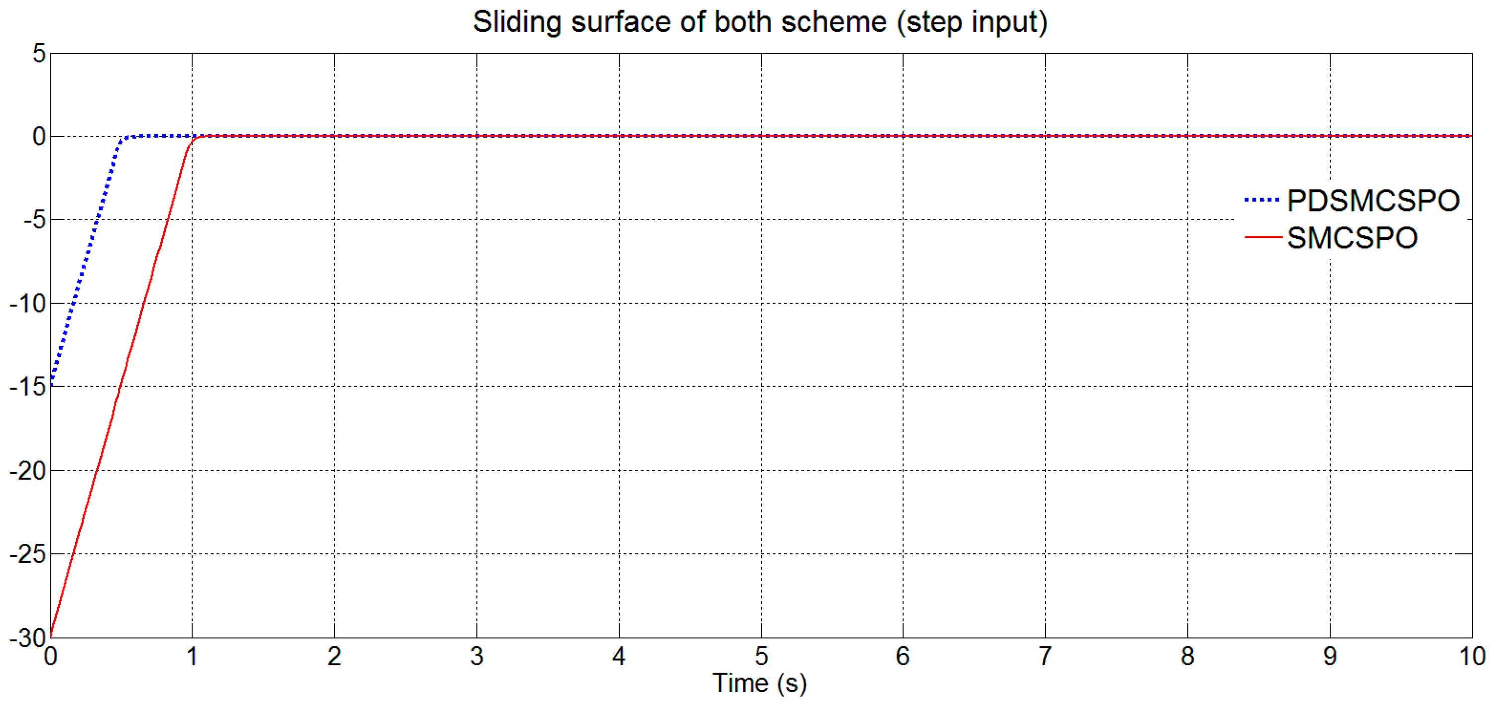
3.2.3. Step Output
3.2.4. Sliding Surface Response
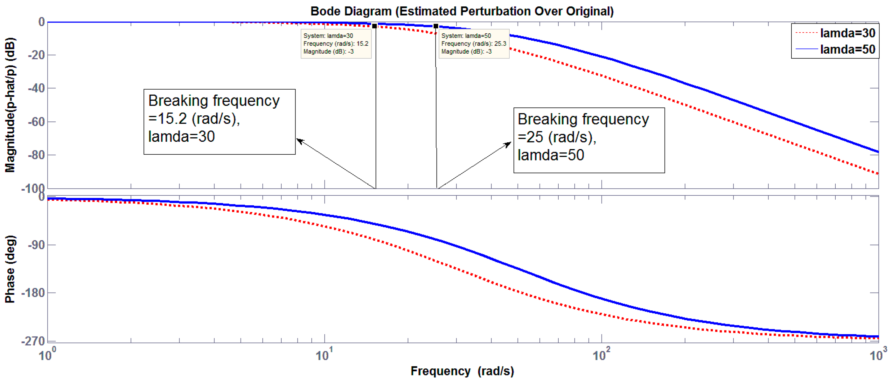
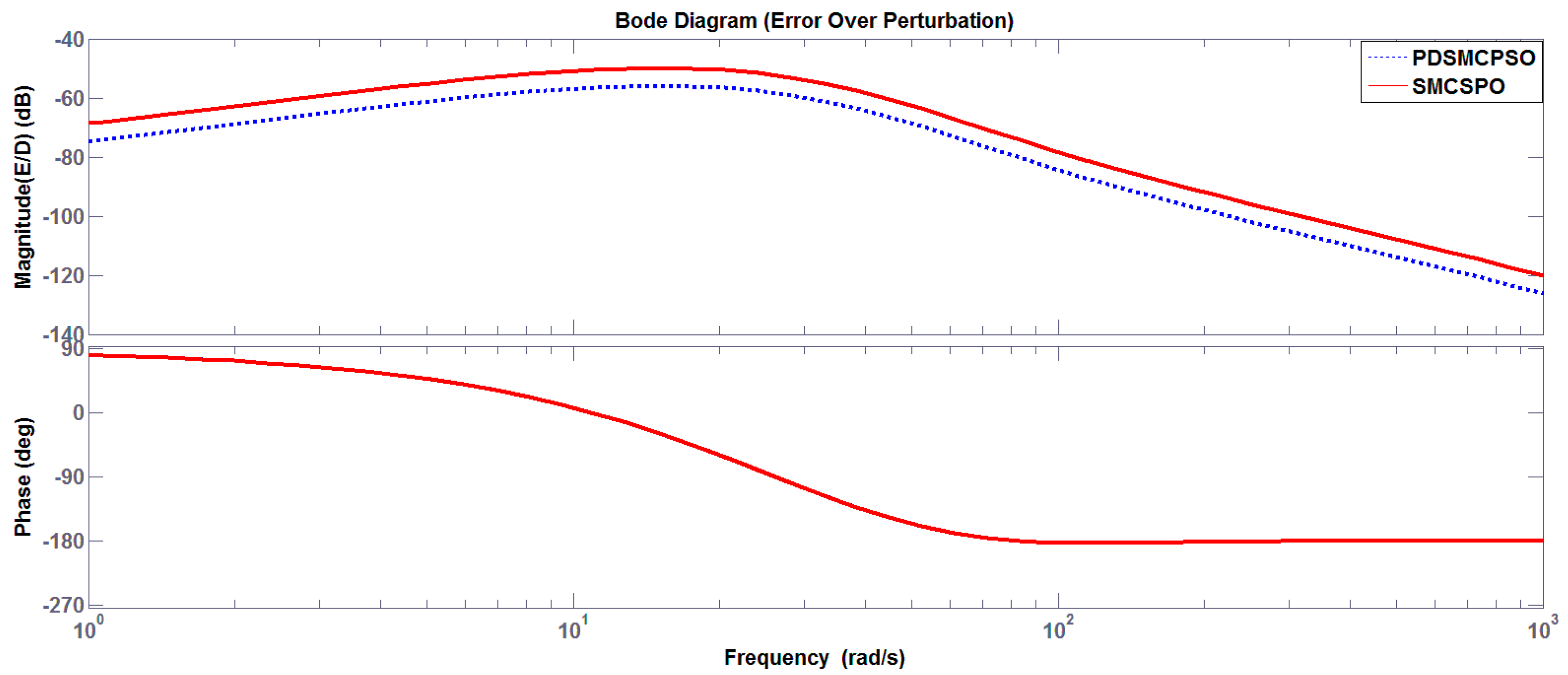
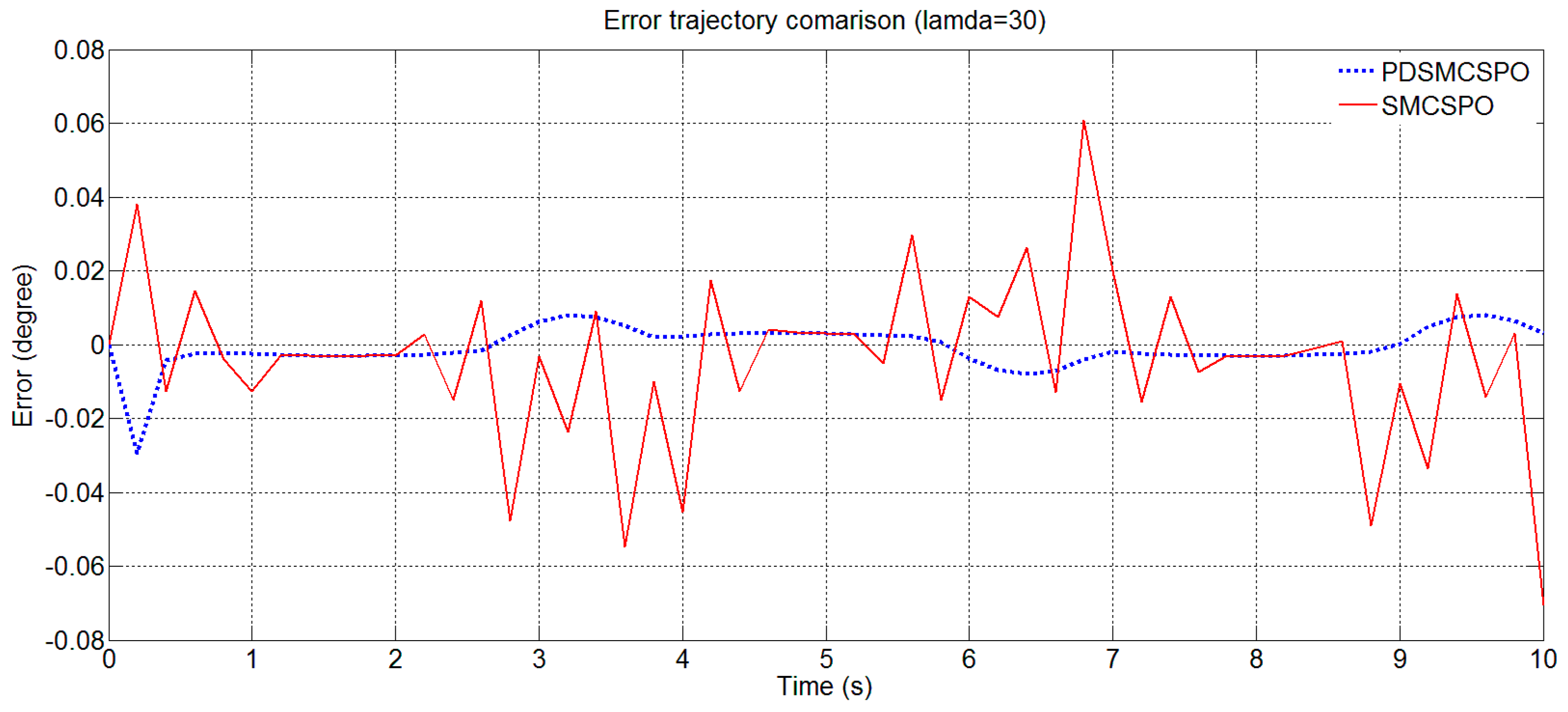
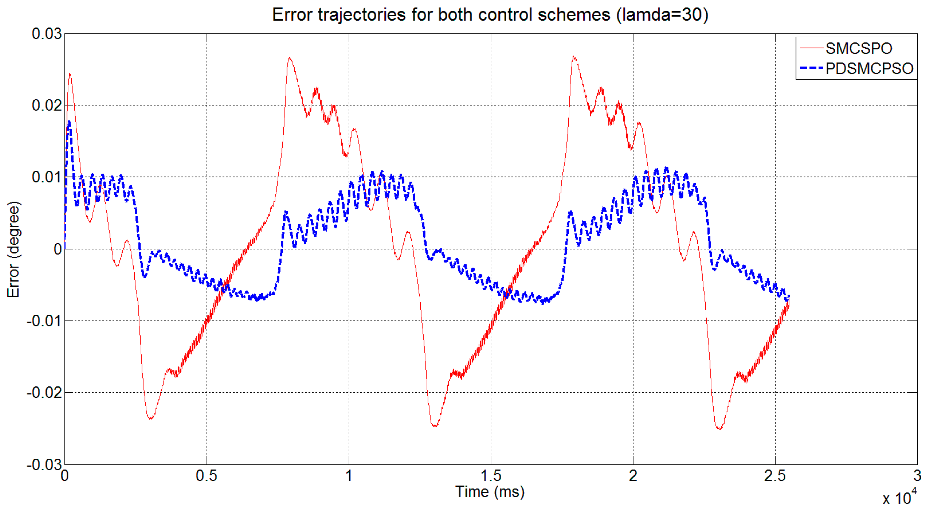
3.2.5. Output Error over Perturbation
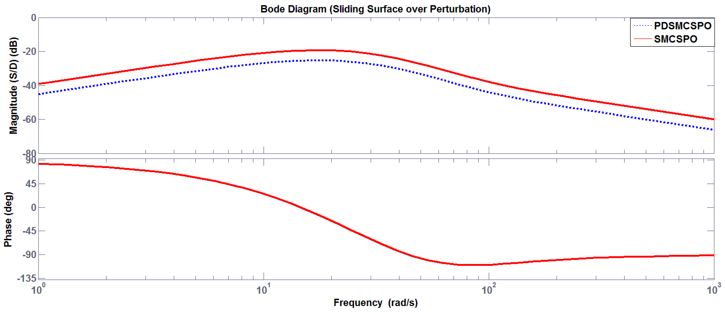
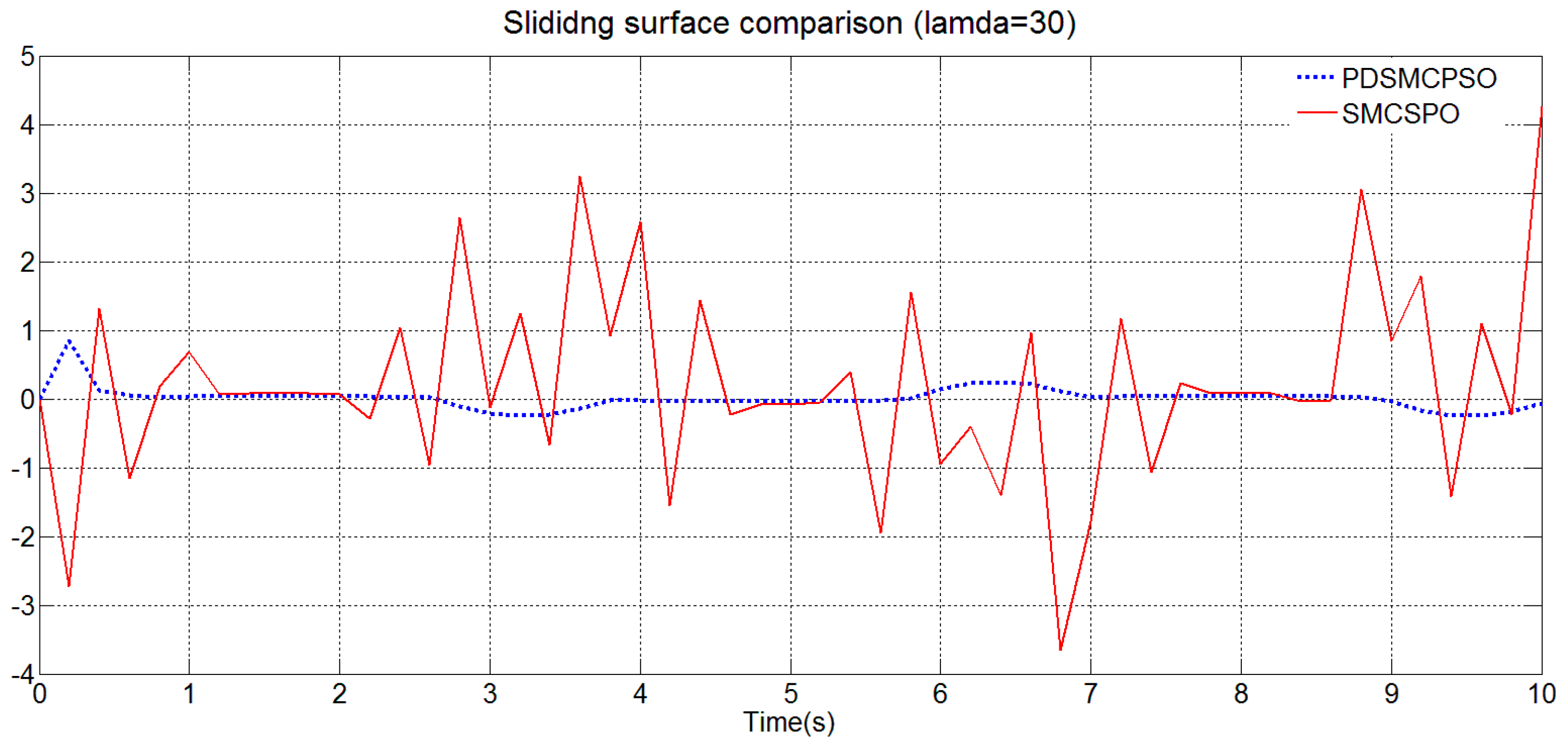
3.2.6. Sliding Surface over Perturbation
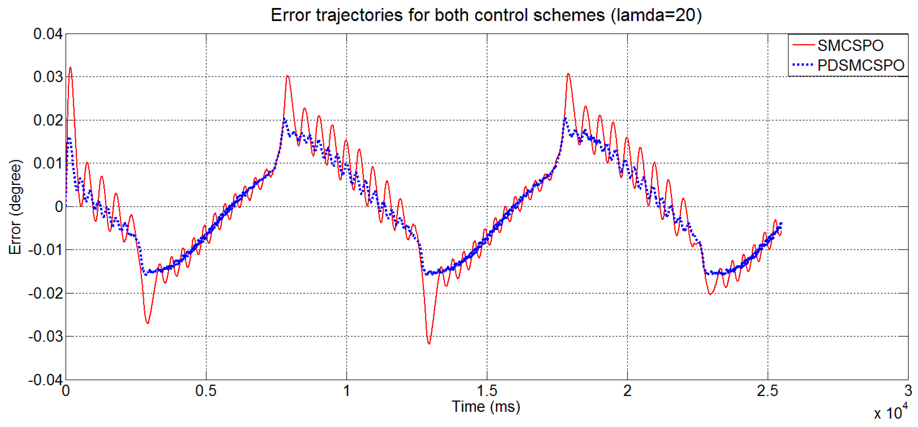
3.3. Experimental Results
4. Conclusions
Author Contributions
Funding
Acknowledgments
Conflicts of Interest
References
- Reuters, Global News, Adivision of Corus Entertainment Inc. Available online: https://globalnews.ca/news/3286191/robots-to-play-key-role-in-dismantling-nuclear-reactors-at-fukushima (accessed on 14 November 2018).
- Jie, W.; Kallu, K.D.; Kim, H.H.; Lee, M.C. TSMCSPO based position control for a hydraulic manipulator. In Proceedings of the 18th International Conferenceon Control, Automation and Systems (ICCAS), Yong Pyong Resort, Pyeong Chang, Korea, 17–20 October 2018. [Google Scholar]
- Truong, D.Q.; Truong, B.N.M.; Trung, N.T.; Nahian, S.A.; Ahn, K.K. Force reflecting joystick control for applications to bilateral teleoperation in construction machinery. Int. J. Precis. Eng. Manuf. 2017, 18, 301–315. [Google Scholar] [CrossRef]
- Peñaloza-Mejía, O.; Márquez-Martínez, L.A.; Alvarez-Gallegos, J.; Alvarez, J. Master-slave teleoperation of under actuated mechanical systems with communication delays. Int. J. Control Autom. Syst. 2017, 15, 827–836. [Google Scholar] [CrossRef]
- Mellah, R.; Guermah, S.; Toumi, R. Adaptive control of bilateral teleoperation system with compensatory neural-fuzzy controllers. Int. J. Control Autom. Syst. 2017, 15, 1949–1959. [Google Scholar] [CrossRef]
- Farooq, U.; Gu, J.; El-Hawary, M.; Asad, M.U.; Abbas, G. Fuzzy model based bilateral control design of nonlinear tele-operation system using method of state convergence. IEEE Access 2016, 4, 4119–4135. [Google Scholar] [CrossRef]
- Kallu, K.D.; Abbasi, S.J.; Yaqub, M.A.; Lee, M.C. Tele-operated bilateral control of hydraulic servo system using estimated reaction for ceofen deffector by SMCSPO. In Proceedings of the 15th International Conference on Ubiquitous Robots and Ambient Intelligence (URAI), Honolulu, HI, USA, 26–30 June 2018. [Google Scholar]
- Lawrence, D.A. Stability and transparency in bilateral teleoperation. IEEE Trans. Robot. Autom. 1993, 9, 624–637. [Google Scholar] [CrossRef]
- Terra, M.J.; Elmali, H.; Olgac, N. Sliding Mode Control with Sliding Perturbation Observer. J. Dyn. Syst. Meas. Control 1997, 119, 657–665. [Google Scholar]
- Elmali, H.; Olgac, N. Sliding mode control with perturbation estimation (SMCPE): A new approach. Int. J. Control 1992, 56, 923–941. [Google Scholar] [CrossRef]
- Slotine, J.J.; Sastry, S.S. Tracking control of nonlinear system using sliding surfaces with application to robot manipulators. Int. J. Control 1983, 38, 465–492. [Google Scholar] [CrossRef]
- Butt, Q.; Bhatti, A.I. Estimation of gasoline-engine parameters using high order sliding mode control. IEEE Trans Ind. Electron. 2008, 55, 3908–3916. [Google Scholar] [CrossRef]
- Young, K.D.; Ozguner, U. Sliding Mode: Control Engineering in practice. In Proceeding of the American Control Conference, San Diego, CA, USA, 2–4 June 1999. [Google Scholar]
- Yan, X.G.; Spurgeon, S.K.; Edwards, C. Introduction. In Variable Structure Control of Complex Systems. Communications and Control Engineering; Springer: Cham, Switzerland, 2017. [Google Scholar]
- Abbasi, S.J.; Kallu, K.D.; Jie, W.; Lee, M.C. Robust control design for 2 link robotic manipulator. In Proceedings of the 13t Korea Robotics Society (KRoC), Gangwon, Korea, 21–24 January 2018. [Google Scholar]
- Abbasi, S.J.; Kallu, K.D.; Lee, M.C. Comparison of robustness of SMC and PD control of 2 link robot manipulator. In Proceedings of the AROB, Busan, Korea, 5–6 September 2017. [Google Scholar]
- Liu, X.; Jiang, W.; Dong, X.C. Nonlinear adaptive control for dynamic and dead zone uncertainties in robotic systems. Int. J. Control Autom. Syst. 2017, 15, 875–882. [Google Scholar] [CrossRef]
- Li, S.; Yang, J.; Chen, W.H.; Chen, X. Genralized Extended State Observer Based Control for System with Mismatched Uncertainties. IEEE Trans. Ind. Delect. 2012, 59, 4792–4802. [Google Scholar] [CrossRef]
- Guo, B.Z.; Zhao, Z.L. Extended State Observe for Nonlinear System with Uncertanity; IFAC: Milano, Italy, 2011. [Google Scholar]
- Jie, W.; Kallu, K.D.; Lee, M.C. A reaction force estimation method of end effector of two link manipulator using SMCSPO. In Proceedings of the 13th International Conference on Ubiquitous Robots and Ambient Intelligence (URAI), Xian, China, 19–22 August 2016. [Google Scholar]
- Kallu, K.D.; Jie, W.; Lee, M.C. PDSPO based estimation of reaction force of end effector of two link manipulator without sensor. In Proceedings of the Society of Instrument and Control Engineers (SICE), Tsukuba, Japan, 2023 September 2016. [Google Scholar]
- Kallu, K.D.; Jie, W.; Lee, M.C. Sensorless reaction force estimation of the end effector of a dual-arm robot manipulator using Sliding Mode Control with Sliding Perturbation Observer. Int. J. Control Autom. Syst. 2018, 16, 1367–1378. [Google Scholar] [CrossRef]
- Kallu, K.; Wang, J.; Abbasi, S.; Lee, M. Estimated reaction force based bilateral control between 3DOF master and hydraulic slave manipulators for dismantlement. Electronics 2018, 7, 256. [Google Scholar] [CrossRef]
- Abbasi, S.J.; Kallu, K.D.; Lee, M.C. Efficient control of non-linear system using modified sliding mode control. In Proceedings of the Society of Instrument and Control Engineers (SICE), Nara, Japan, 11–14 September 2018. [Google Scholar]
- Lee, M.C.; Aoshima, N. Identification and its evaluation of the system with an on linear element by signal compression method. Trans. Soc. Instrum. Control Eng. 1989, 25, 729–736. [Google Scholar] [CrossRef]


| Serial No | Moment of Inertia () | Damper () |
|---|---|---|
| 1 | 303 | 15,355 |
| Serial. NO | SMC | PDSMC |
|---|---|---|
| 1 | K = 550 | K = 275 |
| 2 | C = 16 | |
| 3 | D = 500 | D = 500 |
| 4 | Step input | Step input |
| Serial. No | SMC | PDSMC | Disturbance |
|---|---|---|---|
| 1 | affected | affected | D < 275 (rad/s) |
| 2 | affected | not affected | 275 < D <550 |
| 3 | not affected | not affected | D > 550 |
| Serial. No | SMCSPO | PDSMCSPO |
|---|---|---|
| 1 | ||
| 2 | ||
| 3 | ||
| 4 | ||
| 5 | ||
| 6 | ||
| 7 | ||
| 8 | Input = step | Input = step |
© 2019 by the authors. Licensee MDPI, Basel, Switzerland. This article is an open access article distributed under the terms and conditions of the Creative Commons Attribution (CC BY) license (http://creativecommons.org/licenses/by/4.0/).
Share and Cite
Abbasi, S.J.; Kallu, K.D.; Lee, M.C. Efficient Control of a Non-Linear System Using a Modified Sliding Mode Control. Appl. Sci. 2019, 9, 1284. https://doi.org/10.3390/app9071284
Abbasi SJ, Kallu KD, Lee MC. Efficient Control of a Non-Linear System Using a Modified Sliding Mode Control. Applied Sciences. 2019; 9(7):1284. https://doi.org/10.3390/app9071284
Chicago/Turabian StyleAbbasi, Saad Jamshed, Karam Dad Kallu, and Min Cheol Lee. 2019. "Efficient Control of a Non-Linear System Using a Modified Sliding Mode Control" Applied Sciences 9, no. 7: 1284. https://doi.org/10.3390/app9071284
APA StyleAbbasi, S. J., Kallu, K. D., & Lee, M. C. (2019). Efficient Control of a Non-Linear System Using a Modified Sliding Mode Control. Applied Sciences, 9(7), 1284. https://doi.org/10.3390/app9071284