Recent Advances in DSP Techniques for Mode Division Multiplexing Optical Networks with MIMO Equalization: A Review

Abstract

This paper provides a technical review regarding the latest progress on multi-input multi-output (MIMO) digital signal processing (DSP) equalization techniques for high-capacity fiber-optic communication networks. Space division multiplexing (SDM) technology was initially developed to improve the demanding capacity of optic-interconnect links through mode-division multiplexing (MDM) using few-mode fibers (FMF), or core-multiplexing exploiting multicore fibers (MCF). Primarily, adaptive MIMO filtering techniques were proposed to de-multiplex the signals upon different modes or cores, and to dynamically compensate for the differential mode group delays (DMGD) plus mode-dependent loss (MDL) via DSP. Particularly, the frequency-domain equalization (FDE) techniques suggestively lessen the algorithmic complexity, compared with time-domain equalization (TDE), while holding comparable performance, amongst which the least mean squares (LMS) and recursive least squares (RLS) algorithms are most ubiquitous and, hence, extensively premeditated. In this paper, we not only enclose the state of the art of MIMO equalizers, predominantly focusing on the advantage of implementing the space–time block-coding (STBC)-assisted MIMO technique, but we also cover the performance evaluation for different MIMO-FDE schemes of DMGD and MDL for adaptive coherent receivers. Moreover, the hardware complexity optimization for MIMO-DSP is discussed, and a joint-compensation scheme is deliberated for chromatic dispersion (CD) and DMGD, along with a number of recent experimental demonstrations using MIMO-DSP.

1. Introduction

The space division multiplexing (SDM) systems were proposed to improve the capacity of fiber-optic transmission links, either by means of core multiplexing exploiting multicore fibers (MCF), or with mode-division multiplexing (MDM) using few-mode fibers (FMF) [1,2,3]. Device integration is the most likely approach to accomplish power consumption and cost reduction, through a variety of proposals for realizing parallel spatial channels, including integrating parallel transmitters, receivers, and amplifiers in the same device, as well as utilizing various multimode or multicore fibers, as shown in Figure 1 [4].

Amongst these proposals, the simplest solution is to solely apply fiber bundles to have the same behavior as N single-mode fibers, which can consist of a fiber ribbon or a multi-element fiber as displayed in Figure 1a. Such a multi-element fiber provides a smooth upgrade path where all existing components can be reused, and the power consumption and cost go up with the scale of the fiber bundles. In contrast, MCFs epitomize the next step in parallel fiber integration, where the adjacent fiber cores are enclosed in the same glass cladding, and it allows novel system architectures such as local oscillator sharing with less temperature-dependent fluctuation, as revealed in Figure 1b. It is worth mentioning that MCFs are usually designed with low inter-core cross-talk; thus, multiple-input multiple-output (MIMO) digital signal processing (DSP) is not required at the receiver. On the other hand, mode coupling is difficult to avoid in FMFs and, hence, necessitates the usage of MIMO DSP in the SDM systems, where orthogonal spatial modes within the same fiber core form the parallel channels, as exposed in Figure 1c. Furthermore, strongly coupled MCFs that behave like FMFs were also proposed with certain combined advantages, which shows there is great potential to combine MCF with few-mode cores in next-generation optical-fiber communication systems [5,6].

Principally, the adaptive multi-input multi-output (MIMO) frequency-domain equalization (FDE) techniques were recognized to de-multiplex the signals upon diverse modes, as well as compensate for the differential mode group delay (DMGD) dynamically through digital signal processing (DSP) [7,8,9]. The FDE techniques can reduce the algorithmic complexity evocatively, in comparison with the time-domain equalization (TDE), while holding equivalent performance, amongst which the least mean squares (LMS) and recursive least squares (RLS) algorithms are most widely held and, hence, broadly studied [10,11,12]. Although the LMS approach has lower complexity, it suffers from severe performance deprivation and exhibits slower convergence, while encountering a large number of parameters to be simultaneously adapted in future SDM channels [13]. Alternatively, faster convergence can be accomplished by applying RLS with a more sophisticated algorithmic conformation at the price of higher complexity [14,15]. Hereafter, it is significant to develop a MIMO-DSP FDE algorithm with the intention of achieving an RLS-level performance at an LMS-adapted complexity for an SDM-based optical communication system.

Another bewildering deficiency of FMF-based optical fiber systems is the mode-dependent loss (MDL), which soars from inline component defectiveness and disorders the modal orthogonality, consequently degrading the overall capacity of MIMO channels [16]. With the aim of lessening the impact of MDL, old-fashioned tactics take account of mode scrambler and specialty fiber designs. These approaches were primarily disadvantaged with high cost, yet they cannot utterly eradicate the accumulated MDL in optical links [17]. Furthermore, the space–time trellis codes (STTC) were proposed to reduce the MDL, but they suffered from great complexity as well [18]. Henceforward, MDL is categorically another key challenge that needs to be triumphed for next-generation optical transmission systems.

The spatial multiplicity versus the transmission distance accomplished in recent SDM- wavelength division multiplexing (WDM) transmission experiments is plotted in Figure 2 [19], where the region with a spatial multiplicity over 30 is designated as the “DSDM region”. The dots in Figure 2 represent the cases of multimode fiber (MMF), MCF, and coupled-core fibers (only three-core and six-core), as well as the latest multicore multimode fiber experiments [20].

The outline of this review article is sketched as follows: Section 2 describes the principles of MIMO equalizers, the LMS and RLS techniques, and the space–time block-coding (STBC) assisted RLS algorithms, while Section 3 introduces the configuration of a typical multimode coherent transmission system transmission system with FMFs for high-order modulation formats. In Section 4, the performance analysis of various adaptive filtering schemes is presented for quadrature phase shift keying (QPSK), 16 quadrature amplitude modulation (16QAM), and 64QAM, correspondingly. Then, Section 5 explores the STBC-based enhancement amongst different modulation formats. In Section 6, we further investigate the bit error rate (BER) versus optical signal-to-noise ratio (OSNR) curves of mode-dependent loss equalization. Last but not least, Section 7 demonstrates the complexity optimization using the proposed single-stage architecture. Finally, Section 8 provides a summary of recent expressive experiments of SDM transmission using MIMO DSP for short-, medium- and long-haul distances.

2. Principle

This section introduces the theoretical background of MIMO equalizers, including LMS, RLS, and the space–time block-coding (STBC) algorithm for SDM optical transmission. Moreover, we also cover the aspects of polarization-related dynamic equalization, orthogonal frequency-division multiplexing (OFDM) FDE requirements, and the MIMO hardware requirements in this section. Although hypothetically any modal cross-talk can be electronically managed by DSP, the algorithmic complexity of the MDM coherent receiver remains one of the main limiting factors to the MIMO equalization scheme. In general, the total complexity of the DSP algorithm can be measured by the number of complex multiplications per symbol per mode, for the reason that the complex multipliers are usually the most resource-consuming arithmetic logics in terms of power consumption, area, and cost in application-specific integrated circuit (ASIC) design [21].

2.1. MIMO Equalizers: State of the Art

Although the SDM conception was present for quite a long time, the real SDM transmission systems were not pursued in industry until recent years [22]. This is because, in MDM systems, it is assumed that signals could be immaculately conveyed under a particular mode without interfering with other spatial channels within an ideal FMF; however, in reality, that might not be the case, for the signals in numerous modes are often cross-coupled to each other due to bending, twisting, and/or fiber fabrication imperfections; henceforward, the orthogonality of modes might only be preserved for a very short distance in industrial SDM applications.

In order to resolve such issue, MIMO signal processing was developed to undo channel cross-talk and recover the transmitted data quality. The coherent receiver structure for a single-carrier system with a 6 × 6 MIMO FDE is exemplified in Figure 3, where the coefficient adaptation can be accomplished with LMS or RLS algorithms along with data-aided training.

The conventional time-domain equalization (TDE) uses a finite impulse response (FIR) filter matrix adapted by the LMS algorithm. The complexity for the TDE ${\mathrm{C}}_{TDE}$ is given by [23]

$$C_{TDE}=3·m·\Delta {\beta }_1·L·R_S,$$

(1)

where $\Delta {\beta }_1$ indicates the DMGD of the fiber, $m$ signifies the number of modes within the fiber, $L$ represents the length of the fiber, and $R_S$ denotes the symbol rate. Subsequently, the complexity of TDE scales linearly with the mode group delay of the optical link, the number of modes, and the symbol rate. Meanwhile, the complexity for FDE ${\mathrm{C}}_{\mathrm{FDE}}$ can be written in the form of

$${\mathrm{C}}_{FDE}=4·\left(m+1\right)·{\log }_2\left(2·\Delta {\beta }_1·L·R_S\right)+8·m.$$

(2)

It can be resolved from the equations above that FDE might substantially reduce the complexity compared with TDE. Characteristically, a block length equal to twice the equalizer length is applied for the adaptive FDE. By dint of even and odd sub-equalizers, an equivalent half-symbol period delay spacing finite impulse response (FIR) filter can be realized in the frequency domain. The required MIMO equalizer duration to compensate for DMGD in the weak-coupling regime can be transcribed as

$${\mathrm{N}}_{DMGD}=⎡\Delta {\beta }_1·L·R_{OS}·R_S⎤,$$

(3)

where $⎡\dots ⎤$ means the ceiling function, ${\Delta \mathsf{\beta }}_1$ signifies the DMGD in the fiber, and ${\mathrm{R}}_{\mathrm{OS}}$ represents the oversampling rate. Furthermore, the MDL can be expressed as [24]

$$\mathrm{MDL}=\underset{k=1~N}{\max }\left({\lambda }_k{}^2\right)/\underset{k=1~N}{\min }\left({\lambda }_k{}^2\right),$$

(4)

where ${\mathsf{\lambda }}_{\mathrm{k}}$ stands for singular values of the coupler transfer matrix, which can be calculated by employing the singular value decomposition (SVD).

To achieve the MIMO equalization, the impulse-response matrix measurement needs to be performed first. An example of the squared magnitude of the polarization-division multiplexing (PDM) SDM 6 × 6 impulse responses for 96 km of a six-mode FMF is depicted in Figure 4, where the columns correspond to the transmitted ports and the rows correspond to the received ports [25]. In Figure 4, the sharp peaks in the subplots identify the main coupling points evidently, which are divided into four regions designated with A (the coupling between the polarization modes LP_01x and LP_01y), B (the coupling between the spatial and polarization modes LP_11ax, LP_11ay, LP_11bx, and LP_11by), and C and D (the cross-talk between LP₀₁ and LP₁₁ modes). Such channel estimation provides a clear picture of the cross-talk introduced by the mode multiplexer and the propagation through the six-mode FMF, which allows a better understanding of the MIMO DSP performance.

Furthermore, a typical eye diagram is shown below of two de-correlated 12.5-Gbps NRZ 2⁷-1 pseudorandom binary sequences (PRBSs) launched into one fundamental mode LP₀₁ and a higher-order LP₁₂ mode, with power adjusted such that both channels received the same power of −12 dBm at the receiver, with decent isolation, low los,s and minimal modal mixing [26]. Consequently, we can observe any substantial coupling between the modal groups within the FMF which would easily close the eye at the receiver. The eye diagram with heavy modal dispersion can be seen in Figure 5b, while the eyes of multiplexing independent channels LP₀₁ and LP₁₂ are displayed in Figure 5c,d.

2.2. LMS and RLS Techniques

Both LMS and RLS algorithms are intended to iteratively minimalize the squared error at all discrete frequencies. The LMS algorithm stands as a stochastic gradient descent minimization using instantaneous error estimates, with the corresponding weight update as [27]

$$W\left(k+1\right)=W\left(k\right)+\mu \left[U\left(k\right)-W\left(k\right)V\left(k\right)\right],$$

(5)

where $\mathrm{W}\left(k\right)$ signifies the MIMO channel matrix vector at frequency $k$, $\mathrm{U}\left(k\right)$ indicates fast Fourier transform (FFT) of detected data blocks, $\mu$ denotes the step size, and $\mathrm{V}\left(k\right)$ represents the FFT of sampled received signals.

In conventional LMS, the convergence rate and equalization performance depend on the same value of the scalar step size $\mathsf{\mu }$. The convergence speed can be enlarged by choosing an adaptive step size based on the power spectral density (PSD) of input signal, which can be conveyed as [28]

$$\mu \left(k\right)=\frac{\mathsf{\alpha }}{\mathrm{S}\left(k\right)},$$

(6)

where S(k) signifies the PSD of a posterior error block, and α symbolizes the adaptation rate, which determines both the convergence speed and equalization performance of the noise PSD directed (NPD) LMS algorithm. The basic schematic of an MDM transmission system using the LMS algorithm is shown in Figure 6.

In contrast, the RLS algorithm depends on the iterative minimization of an exponentially weighted cost function, whose convergence speed is not strongly dependent on the input statistics, with the corresponding weight update as

$$\mathrm{W}\left(k+1\right)=\mathrm{W}\left(k\right)+\left[\mathrm{U}\left(k\right)-\mathrm{W}\left(k\right)\mathrm{V}\left(k\right)\right]·\mathrm{V}{\left(k\right)}^H·\left[\mathrm{R}\left(k\right)·{\beta }^{-1}\right],$$

(7)

where $\mathrm{R}\left(\mathrm{k}\right)$ symbolizes a tracked inverse time-averaged weighted correlation matrix, the superscript H signifies the Hermitian conjugate, and $\mathsf{\beta }$ denotes a forgetting factor, which gives an exponentially lower weight to older error samples. Consequently, the main difference between the conventional LMS and RLS algorithms is that RLS has a growing memory due to $\mathrm{R}\left(\mathrm{k}\right)$ and $\mathsf{\beta }$, and, thus, might achieve an even lower OSNR and faster adaptation. Specifically, the tracked inverse time-averaged weighted correlation matrix can be denoted as [29]

$$R\left(k+1\right)=\left[R\left(k\right)·{\beta }^{-1}\right]-\left\{\frac{\left[R\left(k\right)·{\beta }^{-1}\right]·\mathrm{V}\left(k\right)·\mathrm{V}{\left(k\right)}^H·\left[R\left(k\right)·{\beta }^{-1}\right]}{1+\mathrm{V}{\left(k\right)}^H·\left[R\left(k\right)·{\beta }^{-1}\right]·\mathrm{V}\left(k\right)}\right\},$$

(8)

which assigns a different step size to each adjustable RLS equalizer’s coefficient at their updates, rendering all frequency bins with a uniform convergence speed, thus cultivating the total algorithmic performance.

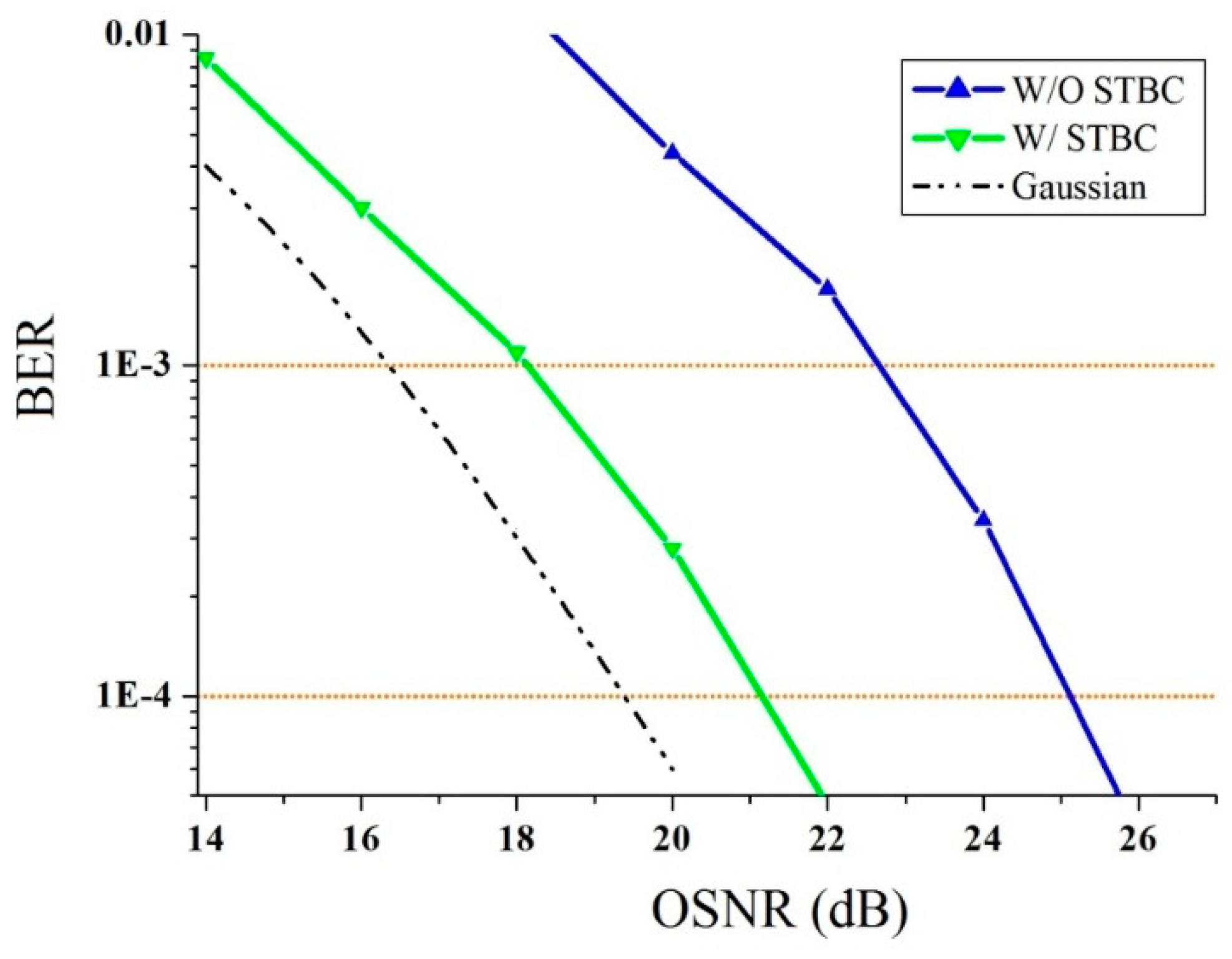
2.3. STBC-Assisted RLS Algorithms

One of the primary issues regarding the conventional RLS implementation might be its comparatively sophisticated computational complexity, attributable to the recursive updating with a growing memory. Henceforth, in order to accomplish a quasi-RLS performance at a quasi-LMS cost, the STBC technique can be applied to aid the RLS approach, which is defined as follows: assuming multiple copies of data stream are transmitted across a number of spatial modes in an FMF transmission, some of the received copies are better than the others under the same scattering, reflection, or thermal noise; thus, the various received versions of the data can be exploited to increase the overall system reliability [30].

The space and time allocation for the STBC-aided RLS algorithm can be briefly represented as shown in Figure 7, as a matrix of spatial channels and time slots, whereby each element is the modulated symbol to be transmitted in mode $i$ at time slot $j$. We may choose different combinations, and we can apply one or more of received copies to properly decode the received signal and, therefore, achieve better performance.

The architecture of the adaptive STBC-RLS equalizer in an $\mathrm{m}$-mode FMF transmission system is illuminated in Figure 8. At coherent detection, the serial-to-parallel (S/P) converters split each data sequence ${\mathrm{y}}_1,\dots {\mathrm{y}}_{\mathrm{m}}$ into even/odd sequences, while two consecutive blocks are concatenated. After the FFT, the samples of the k-th block are overlapped with the ($\mathrm{k}$ − 1)th block at frequency $\mathrm{k}$, which are further alienated into sequential blocks ${\mathrm{y}}_{\mathrm{q}}^{\mathrm{P}}\left(\mathrm{k}\right)$, where superscript P specifies an even or odd sequence. Each block is then converted to the frequency domain with FFT as ${\mathrm{Y}}_{\mathrm{q}}^{\mathrm{P}}\left(\mathrm{k}\right)$, which goes through an inversed channel filter for the data matrix production with the even or odd tributaries, while ${\mathrm{H}}_{\mathrm{q},\mathrm{j}}^{\mathrm{P}}\left(\mathrm{k}\right)$ stands for the inversed channel filter in Jones-vector notation, while both $\mathrm{q}$ and $\mathrm{j}$ denote mode indices between 1 and $\mathrm{m}$. After an adaptive MIMO equalization, the carrier recovery is applied to mitigate the laser phase noise, the outputs of which are transformed back to the time domain using inverse FFT (IFFT), compared to the desired response to generate an error vector, and to update the receiver coefficients in a training mode until they converge. Then, it switches to a decision-directed mode, whereby reconstructed data are transformed back using FFT through the zero padding to update the coefficients [31].

The weight update of the STBC-aided RLS algorithm follows the rules below, whereas the corresponding equalizer coefficients are updated every two blocks ($\mathrm{k}+2$) instead of each block ($\mathrm{k}+1$) in the recursion.

$$\mathrm{W}\left(k+2\right)=\mathrm{W}\left(k\right)+\left(\begin{array}{cc}{\mathrm{P}}_{k+2}& 0\\ 0& {\mathrm{P}}_{k+2}\end{array}\right){\left({\mathrm{U}}_{k+2}\right)}^{*}·\left[{\mathrm{D}}_{k+2}-{\mathrm{U}}_{k+2}·\mathrm{W}\left(k\right)\right],$$

(9)

where ${\mathrm{U}}_{\mathrm{k}+2}$ denotes the Alamouti matrix containing the received symbols from block $\mathrm{k}+2$ and $\mathrm{k}+3$, and ${\mathrm{D}}_{\mathrm{k}+2}$ represents the desired response vector for training and decision-directed tracking [32], while the superscript * indicates the complex conjugation. Meanwhile, the diagonal term ${\mathrm{P}}_{\mathrm{k}+2}$ is given by

$${\mathrm{P}}_{k+2}={\beta }^{-1}·\left[{\mathrm{P}}_k-{\beta }^{-1}·{\mathrm{P}}_k·{\mathsf{\Omega }}_{k+2}·{\mathrm{P}}_k\right],$$

(10)

where $\beta$ is the forgetting factor, and the term ${\mathsf{\Omega }}_{\mathrm{k}+2}$ is given by

$${\mathsf{\Omega }}_{k+2}={\{\mathrm{Diagonal}{[{\left|\mathrm{V}\left(k\right)\right|}^2+{\left|\mathrm{V}\left(k+1\right)\right|}^2]}^{-1}+{\beta }^{-1}·{\mathrm{P}}_k\}}^{-1},$$

(11)

where $\mathrm{V}\left(\mathrm{k}\right)$ stands for the FFT of sampled received signals. By utilizing the STBC scheme, we may choose different combinations, and apply one or more of received copies to correctly decode the received signal, and, thus, attain a better performance. Meanwhile, the STBC is able to accomplish an RLS-level performance with a much lower computational complexity, because no matrix inversion is essential during the recursion. Instead of adding a training sequence to each data block, only a few training blocks are added in the beginning, and the channel variations are tracked at the decision-directed stage in an attempt to reduce the overall system overhead [33].

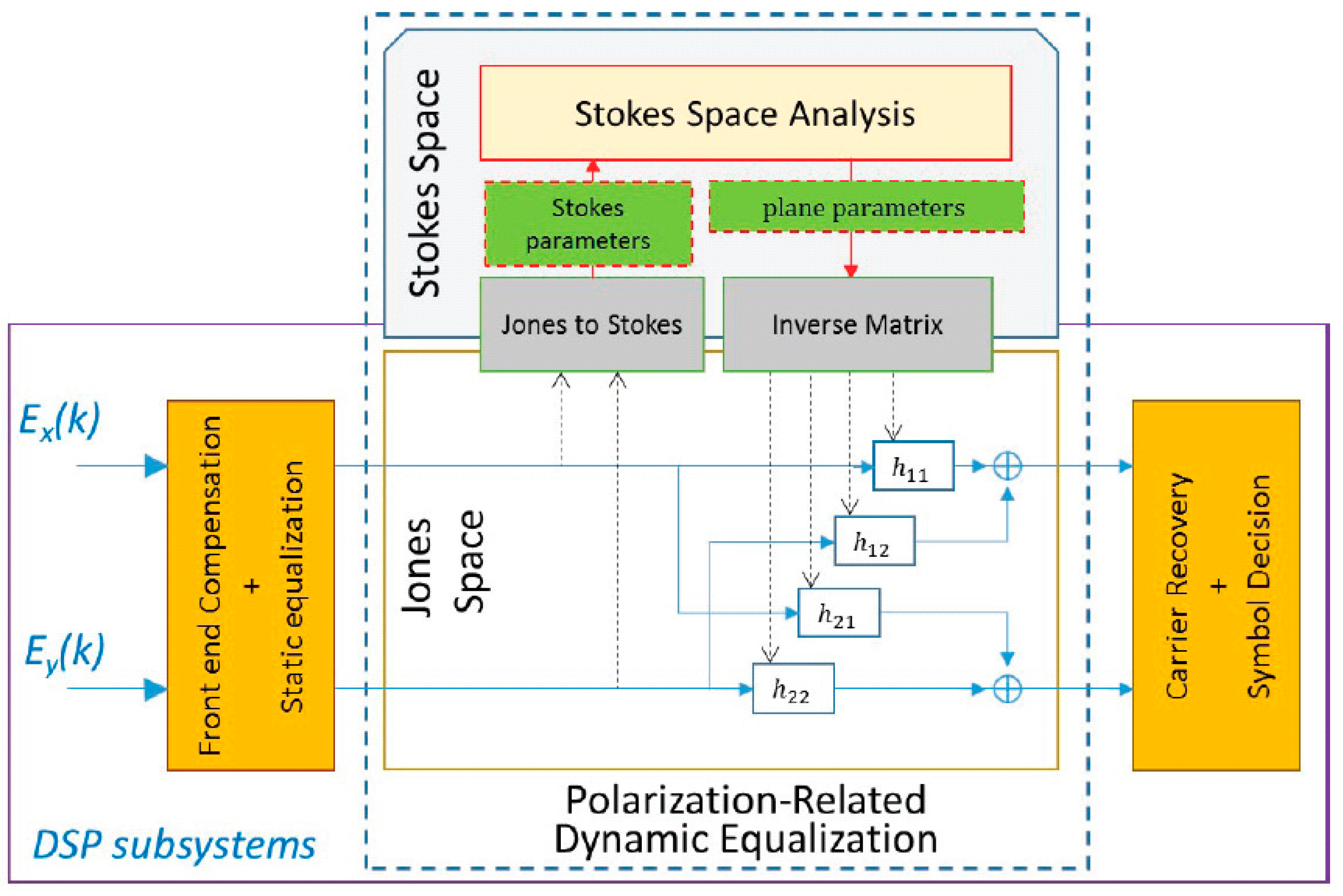
2.4. Polarization-Related Dynamic Equalization

Polarization characterizes a fundamental multiplexing technique, which allows doubling the spectral efficiency of fiber optical transmission systems [34]. To accommodate the usage of two polarization tributaries, polarization de-multiplexing (PolDemux) algorithms represent a crucial part of digital coherent receivers, which makes it conceivable to efficiently compensate for time-varying state of polarization (SOP). The PolDemux approaches include MIMO algorithms such as LMS and RLS, and the constant-modulus algorithms (CMA).

In particular, Stokes space-based DSP techniques improve the polarization de-multiplexing, polarization dependent loss (PDL) compensation, and other polarization-related propagation impairments in coherent receivers, particularly in terms of convergence speed and transparency to higher-level M-ary modulated signals. The block diagram of the DSP subsystems of a coherent transceiver for adaptive equalization of both polarization and phase diversity is presented in Figure 9, which includes the front-end compensation, static equalization, adaptive equalization, carrier phase recovery, and the symbol decision [35].

Furthermore, the Stokes space-based PolDemux method has specific advantages including the higher convergence ratio, the improved robustness against phase noise, and the transparency to higher-level M-ary modulated signals.

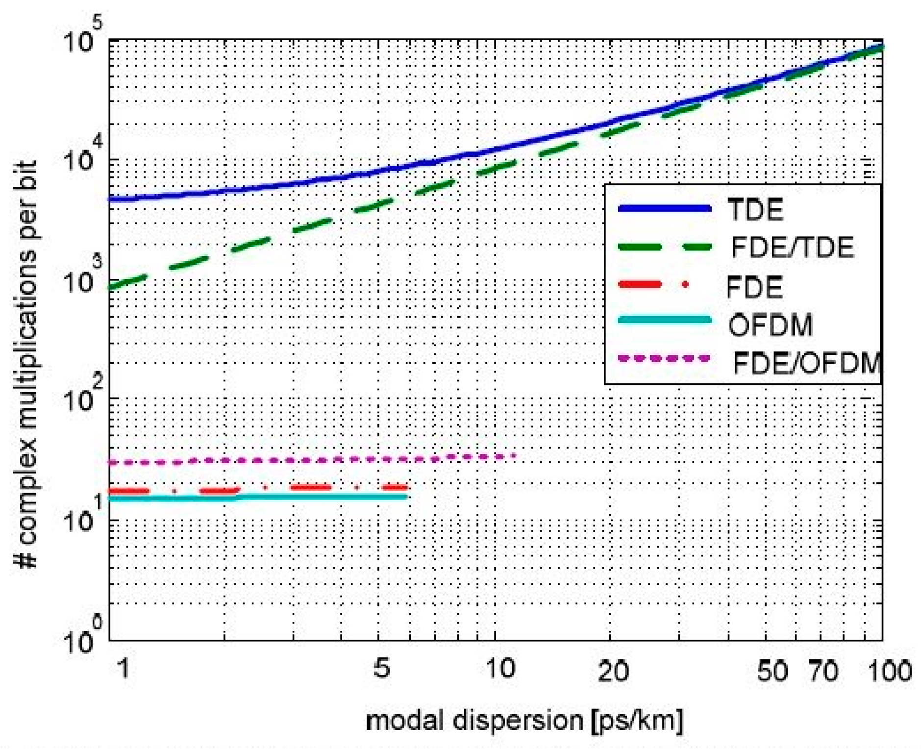
2.5. OFDM FDE Requirements

The high-speed orthogonal frequency-division multiplexing (OFDM) in SDM optical long-haul transmission systems serves as another important aspect of MIMO equalization techniques [36]. The complex multiplications per bit for various equalizer types in terms of modal dispersion for a 2000-km transmission distance and 10 × 10 MIMO is shown in Figure 10, where an FMF with three modes with two polarizations (LP₀₁, LP_11a, LP_11b, LP_21a, LP_21b) results in the number of tributaries being 10.

In principle, the complexity is calculated in a two-dimensional matrix, where one variable is the sampling rate and the other is the size of the FFT. For each configuration, the optimum sampling rate resulting in minimum complexity satisfying the overhead constraint is considered. As we can see, OFDM requires the lowest equalizer complexity for cross-talk compensation in an MDM receiver, for most of the multiplications required for FDE/TDE are caused by time-domain operations. However, OFDM cannot tolerate a modal dispersion of more than 5.9 ps/km modal dispersion due to the 10% overhead constraint for FMF-based optical transmission [37].

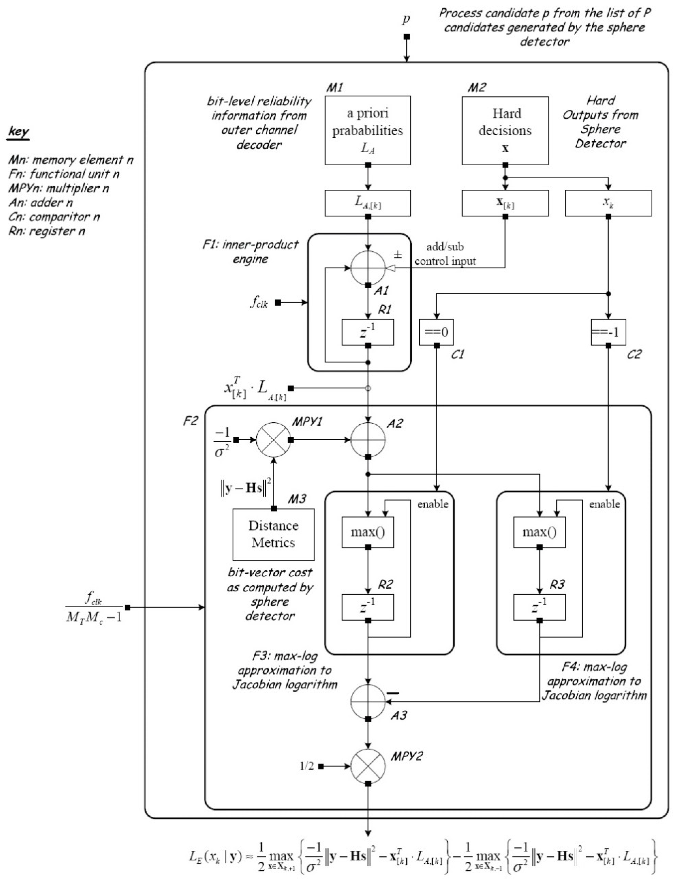
2.6. MIMO Hardware Requirements

Last but not least, this subsection discusses the design and architecture of spatial multiplexing MIMO decoders for field-programmable gate arrays (FPGAs). Conventionally, the optimal hard-decision detection for MIMO systems is the maximum likelihood (ML) detector, which is well known due to its superior performance in terms of BER, but its direct implementation grows exponentially with a higher-level modulation scheme, causing its FPGA implementation to be relatively infeasible [38].

On the other hand, soft-output generation for a sphere detector can solve the ML detection issue in a computationally efficient manner, for a real-time implementation on a DSP processor at high-performance parallel computing platforms. The scalable architecture of soft-output generation for a sphere detector is presented in Figure 11, which requires further micro-architecture optimizations and trade-offs [39].

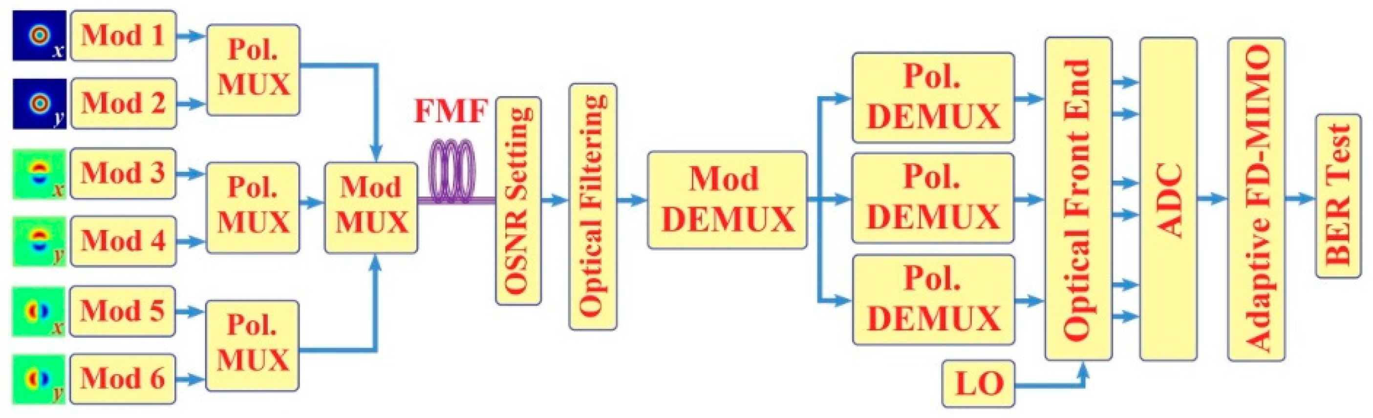
3. System Configuration

The system configuration of a six-mode coherent transmission system is illustrated in Figure 12, with a 2²³ − 1 pseudorandom binary sequence (PRBS) sequence modulated on every mode over a 30-km FMF. The OSNR setting block indicates that the additive white Gaussian noise (AWGN) noise is added after the FMF transmission, while the optical filtering block specifies that a Gaussian filter with a 33-GHz bandwidth is used to suppress the out-of-band noise before the coherent detection.

After mode de-multiplexer (Mod DEMUX), parallel signals are launched into the receiver, and are converted to baseband in the optical front end by internally mixing with the local oscillator (LO) at a linewidth of 100 kHz. The electrical signal in-phase and quadrature (I/Q) components are then re-sampled at two samples per symbol by the analog-to-digital converter (ADC). After the MIMO processing, a BER is estimated for each mode [40].

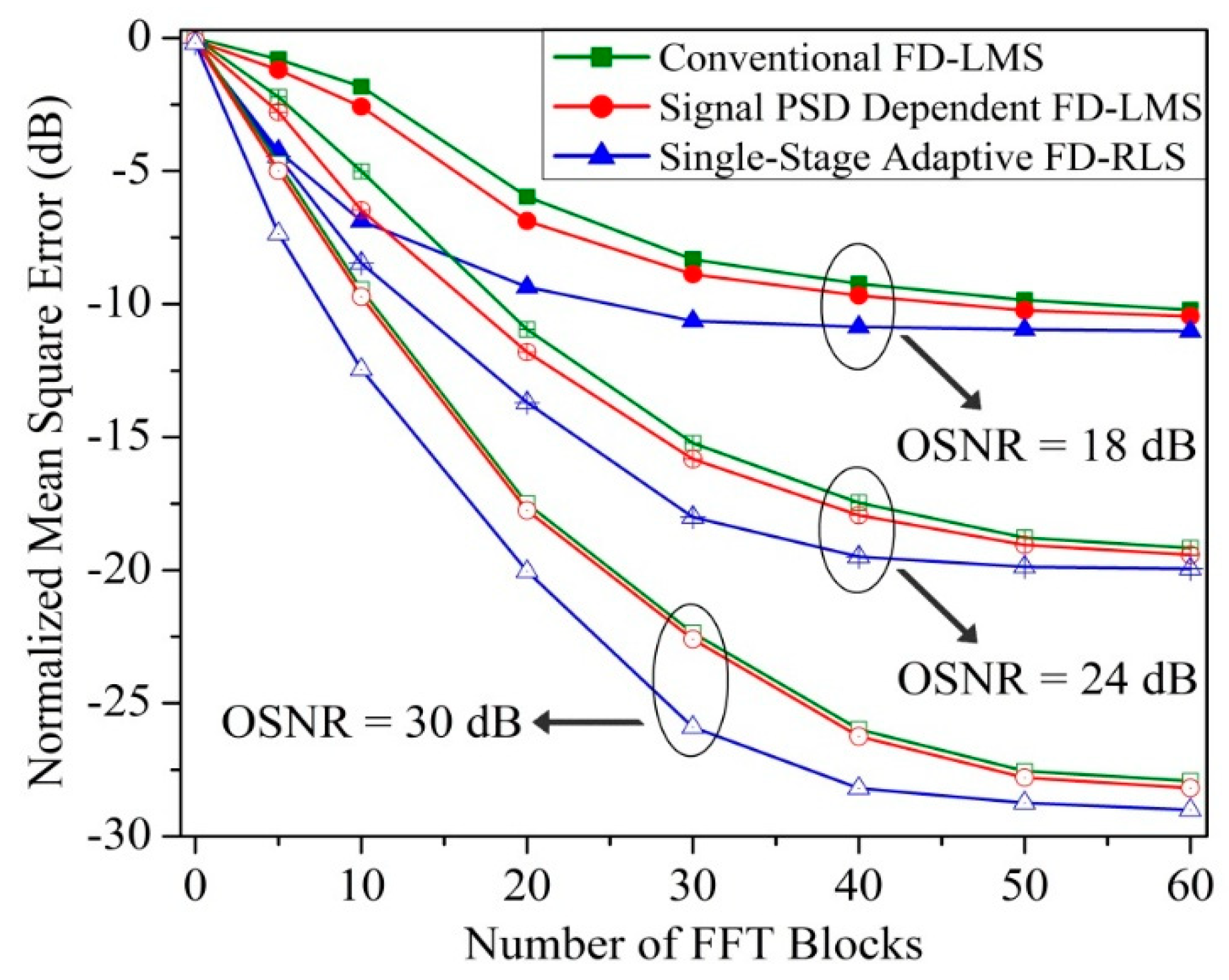
4. Performance Evaluation for Different Adaptive Filtering Schemes

In this section, the convergence speed comparison amongst the conventional LMS algorithm, the noise PSD directed (NPD) LMS algorithm, the RLS algorithm, and the proposed STBC-RLS algorithm for PDM-QPSK signal is exemplified in Figure 13, whereas the normalized mean square error (NMSE) represents the average square errors of each block after the MIMO equalization. The adaptation rate and step size of four algorithms were set to their optimal values; the block length was 8192 samples using 50% overlap with OSNR set at 18 dB. In the meantime, the inset on the right displays the constellation diagram before the STBC compensation, as the received signal was severely distorted, attributable to mode coupling and delay, while the inset on the left indicates the constellation diagram after applying the STBC-RLS compensation, as the modal distortions were remarkably compensated for by the MIMO equalizers over a 30-km FMF.

As for the computational complexity per data symbol for the MIMO FDE, which is mainly determined by the number of complex multiplications, the RLS and LMS algorithms would consume 148 and 302 complex multiplications, respectively, while the proposed STBC-RLS would require 172 complex multiplications, which is roughly a 16.2% increase in hardware complexity compare to LMS, but 75.6% less than that of the RLS approach.

To further upsurge the spectral efficiency of the next-generation SDM transmission systems, the convergence speed comparisons between different algorithms for PDM-16QAM and PDM-64QAM signals are presented in Figure 14 and Figure 15, respectively, whereas the comparison between different modulation formats is summarized in

Table 1. Comparison of multiple modulation formats [21]. QPSK—quadrature phase shift keying; QAM—quadrature amplitude modulation.

Modulation Format	# of Symbols Transmitted	Levels per Carrier	# of Bits per Symbol Contained	Corresponding Data Rate
QPSK	$4=2^2$	2	2	112 Gb/s
16QAM	$16=2^4$	4	4	224 Gb/s
64QAM	$64=2^6$	8	6	336 Gb/s

.

From the plot above, we can see that RLS converges faster to a lower asymptotic NMSE than LMS, because it has a growing memory due to the forgetting factor. The NPD-LMS algorithm can achieve a faster convergence than the traditional LMS, because it adopts variable bin-wise step size to render posterior error of every frequency bin convergent to the background noise of the AWGN channels. Still, the NMSE convergence of the proposed STBC-RLS algorithm seems a bit inferior to that of the conventional RLS in the beginning, for a smaller block size is used for training than the data block size to reduce the system overhead at the expense of a minor loss of performance. Subsequently, to achieve −10 dB steady NMSE, which is equal to a 9.8-dB Q-value, the LMS and NPD-LMS schemes need 55 and 47 FFT blocks, while the RLS and STBC-RLS approaches require roughly 27 and 31 blocks, respectively; henceforward, the convergence rate would be enhanced by 50.9% and 43.6%, respectively.

From the plots, we can see that with higher-order modulation formats, the advantage of RLS convergence rate over that of the LMS becomes even larger, owing to a growing memory, while the difference in NMSE between the proposed STBC-RLS algorithm and the conventional RLS shrinks, which indicates that such proposed adaptive receivers could lower system overhead requirements for higher-order modulation formats.

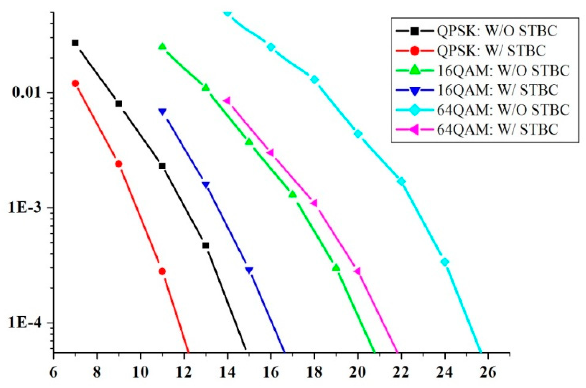
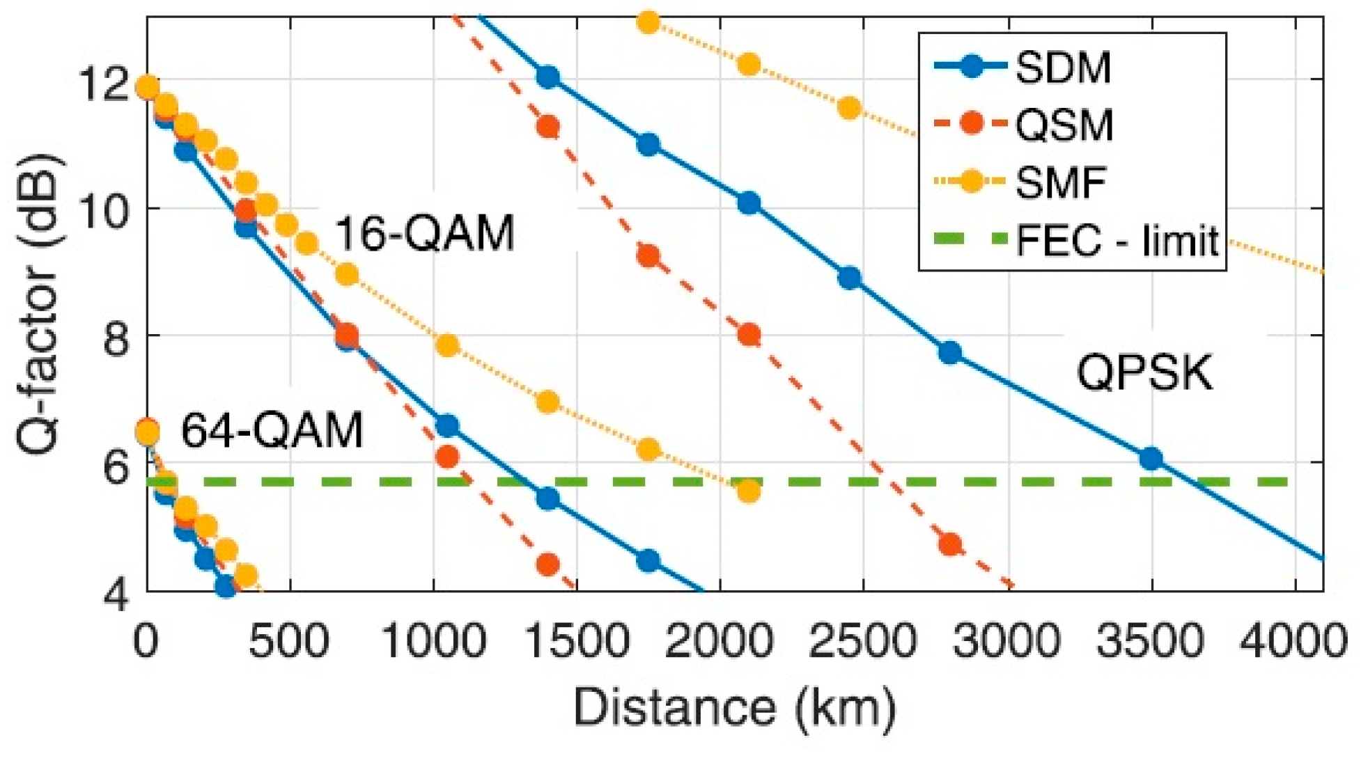
5. STBC-Assisted Improvement between Various Modulation Formats

To irradiate the benefits of using the STBC scheme to mitigate the MDL impairment in the SDM transmission systems, the performance results of the space–time coded FMF transmission with or without using the STBC-RLS scheme are presented in Figure 16, from which we can achieve a roughly 3-dB OSNR improvement for the PDM-QPSK signal at a 10⁻³ BER, whereas the condition for the dotted line marked as Gaussian indicates the performance over a perfect MDL-free Gaussian channel.

Additionally, for the higher-order modulation formats, the performance comparison plots for PDM-16QAM and PDM-64QAM signals with or without using the purposed STBC-RLS scheme are further shown in Figure 17 and Figure 18, respectively.

In summary, the performance comparison for various modulation formats with or without using the STBC-RLS scheme is summarized in Figure 19, whereas the scheme for not using STBC-RLS designates the conventional RLS scheme, from which we can observe that, as more bits per symbol are transmitted, a larger OSNR tolerance improvement could be accomplished by using STBC for higher-order modulation formats. The overall OSNR tolerance can be improved by means of the STBC approach by approximately 3.1, 4.9, and 7.8 dB for QPSK, 16QAM, and 64QAM with respect to BER.

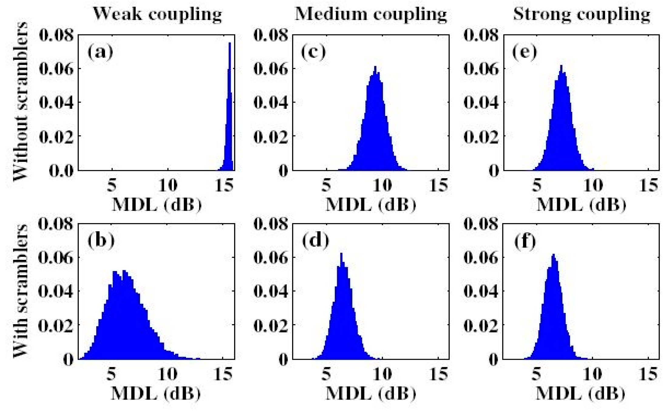
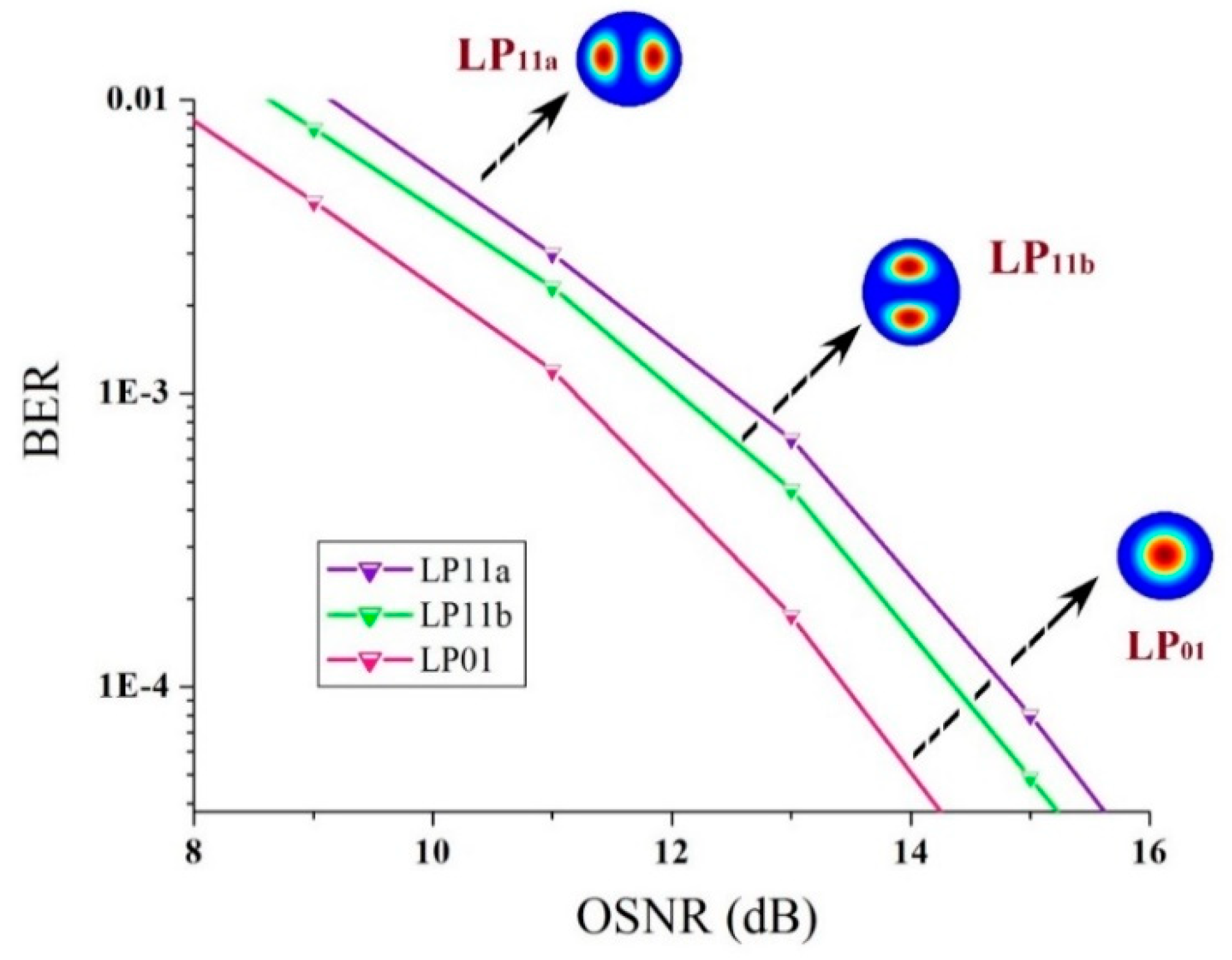
6. MIMO Equalization for Mode-Dependent Loss

The mode-dependent loss (MDL) arises from imperfections in optical components such as optical amplifiers, couplers, and multiplexers, as well as from non-unitary cross-talk in the fiber and at fiber splices and connectors, where the modes experience differential losses or gains when propagating through the optical link, which leads to signal-to-noise ratio disparities along with a loss of orthogonality between modes. The MDL is a capacity-limiting effect reducing the multiplexing benefit of SDM communication systems, which cannot be completely removed at the receiver by simply inserting mode scramblers. The probability distribution functions (PDF) of the accumulated MDL for the different coupling levels, with and without mode scrambling, are shown in Figure 20 as an example [41].

Furthermore, as there are up to three spatial modes being transmitted in our modeling, Figure 21 illustrates the equalization performance of the BER curves at different OSNRs by means of the STBC-RLS algorithm for a PDM-QPSK signal, from which we can see that the BERs of all spatial modes fall after MIMO equalization.

The LP₀₁ mode is able to realize a lower required OSNR for a 10⁻³ BER than the LP₁₁ mode groups, predominantly because its more centralized mode pattern makes the LP₀₁ mode suffer a lesser level of impact from mode coupling and cross-talk. Al though the LP_11a and LP_11b modes share an identical mode pattern as a pair of degenerate modes, their BER performance appears a bit dissimilar triggered by spatial mismatching and rotation. Since we found that the transmitted signals on both x- and y-polarizations provide a comparable performance, here, in these plots, the LP_11b mode is adopted as the average of two orthogonal polarizations for an easier analysis.

Additionally, the BER versus OSNR relationships based on the STBC-RLS algorithm for PDM-16QAM and PDM-64QAM signal compensation for LP₀₁, LP_11a, and LP_11b modes are presented in Figure 22 and Figure 23, respectively. To reach a BER below 10⁻³, the LP₀₁ mode requires a 16.5-dB OSNR, while the LP_11b and LP_11a modes need about 17.7-dB and 18.1-dB OSNRs for the PDM-16QAM signal, while, for the PDM-64QAM signal, the LP₀₁ mode requires a 21.3-dB OSNR, while the LP_11b and LP_11a modes need about 22.8-dB and 23.6-dB OSNRs, respectively.

7. Hardware Complexity Optimization for MIMO

This section focuses on the hardware complexity for MIMO equalization, which includes the FIR filter tap number for MIMO, single-stage architecture, and joint DSP for an MCF-based SDM. For a larger mode number $m$, frequency-domain (FD)-RLS might provide a better performance pertaining to the conventional FD-LMS algorithm, for the convergence speed of FD-RLS is not strongly dependent on the input statistics. Until now, the main issue of the adaptive FD-RLS implementation is its relatively higher computational complexity, due to the recursive updating with a growing memory. In this section, a joint chromatic dispersion (CD) and DMGD optimization technique is proposed for a further reduction in the algorithmic complexity of the FD-RLS approach.

7.1. Filter Tap Number for MIMO

The structure of an MIMO equalizer as an extension of the standard CMA is depicted in Figure 24, which is based on multiple FIR filters in a butterfly structure. The hardware complexity of such an architecture per transmitted bit is only doubled for the 4 × 4 MIMO configuration compared to standard single-mode operation, for sixteen adaptive filters are prerequisite to process 2 × 100 Gb/s with a 4 × 4 MIMO compared to four filters for 1 × 100 Gb/s with a 2 × 2 MIMO as a reference. On the right graph of Q²-factor versus the FIR filter tap number, which is used to estimate the required length of the MIMO equalizer allowing the detection of all the polarization and mode tributaries, an almost flat factor from nine taps to 15 taps can be observed for both 100 Gb/s PDM-QPSK and 2 × 100 Gb/s MDM after a 40-km transmission [42].

The required number of taps per carrier used as a function of distance in recent MDM transmission experiments is illuminated in Figure 25, where the DMGD increases linearly with distance in the weak coupling regime [19]. Fiber management is expedient in decreasing the maximum DMGD in an FMF. In addition, as different forms of signals, fibers, and spatial channels are likely to cohabit in future SDM transport networks, it is also significant that MIMO DSP has sufficient processing capability to handle all received signals.

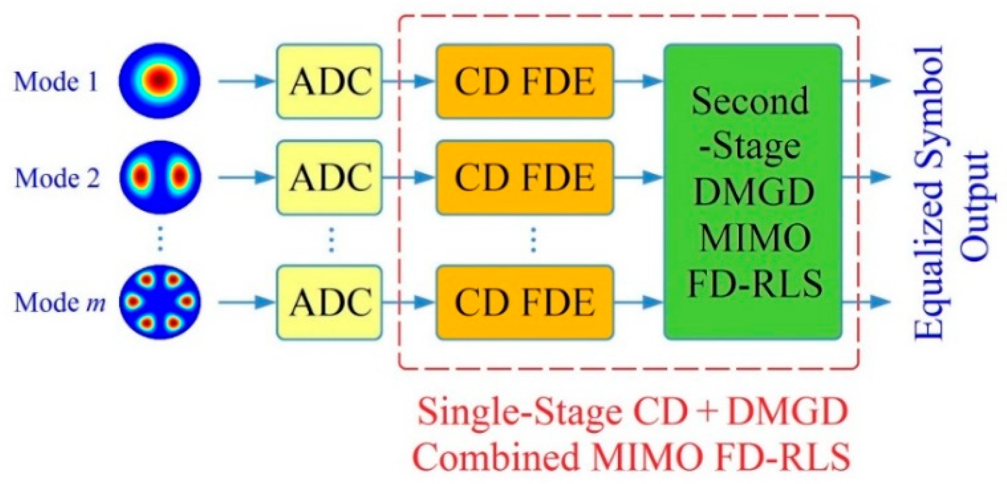
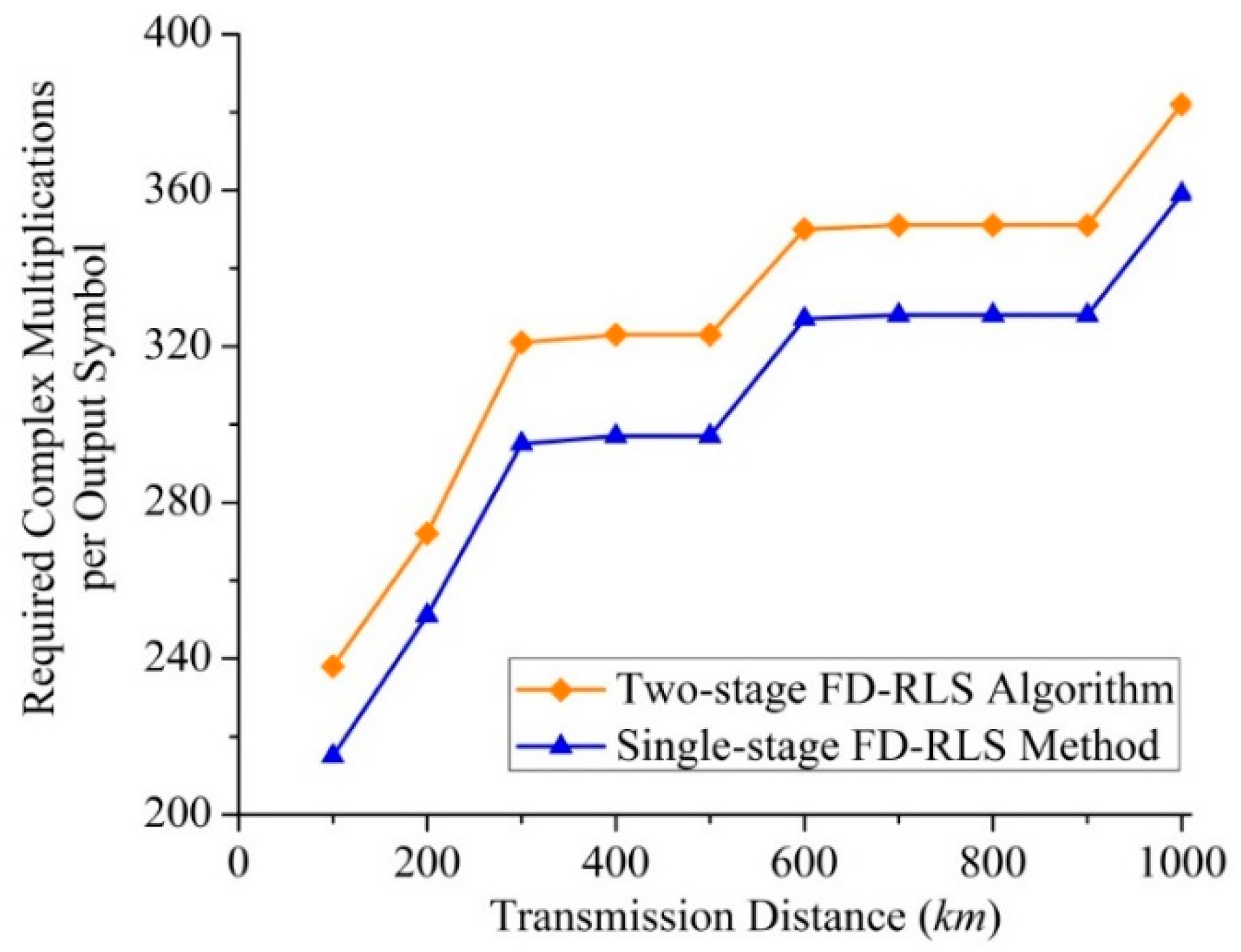
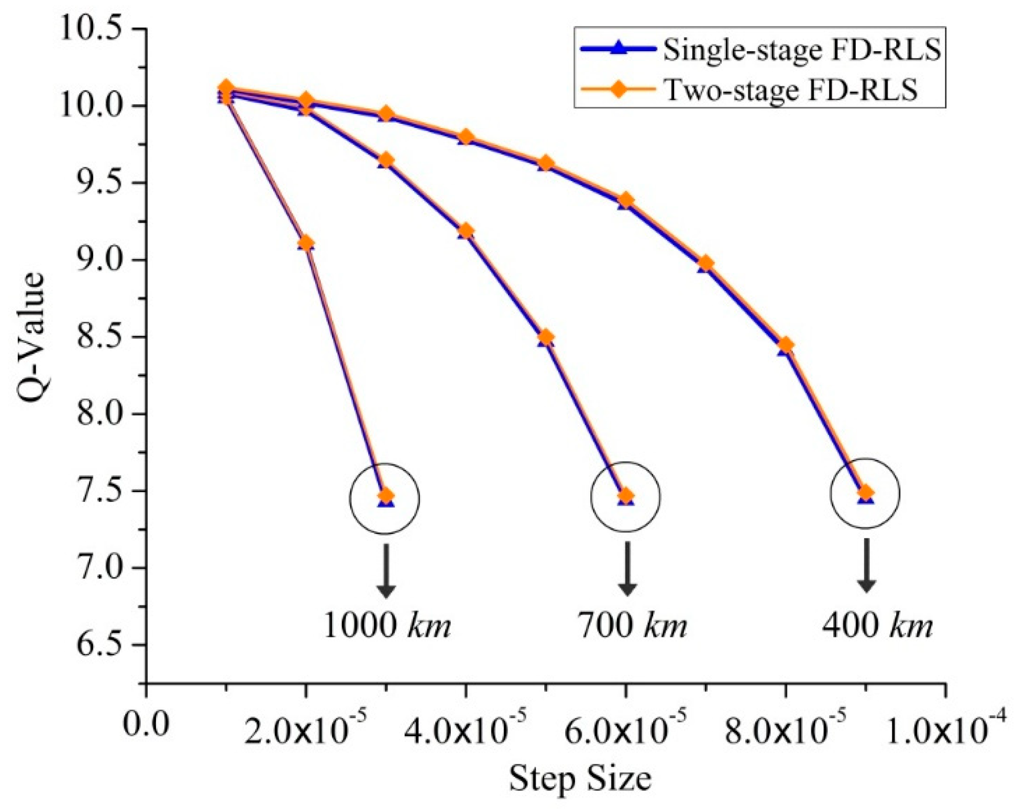
7.2. Single-Stage Architecture

In this subsection, we discuss the complexity optimization using the single-stage architecture of CD and DMGD joint compensation. The equalization of CD and DMGD can be performed together using FFT for efficient implementation of convolution, as a favorable structure for digital coherent receivers, for sparing the CD compensation modules and, hence, reducing the total DSP implementation complexity [43].

The schematic diagram of a coherent receiver for the compensation of the linear channel effects such as CD and DMGD is exemplified in Figure 26. To attain a lower computational complexity, the equalization of CD and DMGD can be implemented together, compared with the conventional two-stage FDE structure, using FFT for an efficient implementation of convolution; thus, $m$ independent static CD compensation modules would be spared. Subsequently, a joint MIMO FDE of the static CD along with the dynamic DMGD would be an auspicious configuration for digital coherent receivers, because it would save a separate CD compensation module, thereby decreasing the total DSP implementation complexity.

Above and beyond, Figure 27 provides the comparison of the required complex multiplications per output symbol at different transmission distances for the two-stage and single-stage FD-RLS algorithms. For a transmission distance rising from 100 km up to 1000 km, the single-stage method continuously consumes fewer complex multiplications than the conventional two-stage method, because both methods use the same FFT size for DMGD compensation for the same transmission distance, whereas the FFT size of static FDE in the two-stage method is determined by the FMF-induced CD. For instance, the two-stage FD-RLS method consumes 323 and 351 complex multiplications per output symbol at 400-km and 800-km transmissions, whereas our proposed single-stage method takes only 297 and 328 complex multiplications per output symbol at the same transmission distances, respectively.

Furthermore, Figure 28 irradiates the Q-value versus the step size of adaptive FD-RLS algorithms in both two-stage and single-stage methods for compensating for DMGD and CD. To attain a <0.5-dB Q-penalty at 400-, 700-, and 1000-km transmissions, the maximum step sizes are 4.5 × 10⁻⁵, 3 × 10⁻⁵, and 1.5 × 10⁻⁵, respectively. In addition, for the same transmission distance, the maximum step sizes required to achieve the same Q-value after equalization are identical for both approaches.

Last but not least, Figure 29 exhibits the convergence speed comparison among three algorithms at different OSNR levels, from which we learnt the time required for convergence grows more slowly for FD-RLS than FD-LMS algorithms as the OSNR increases, equivalent to plummeting the overall training sequence overhead by approximately 30%.

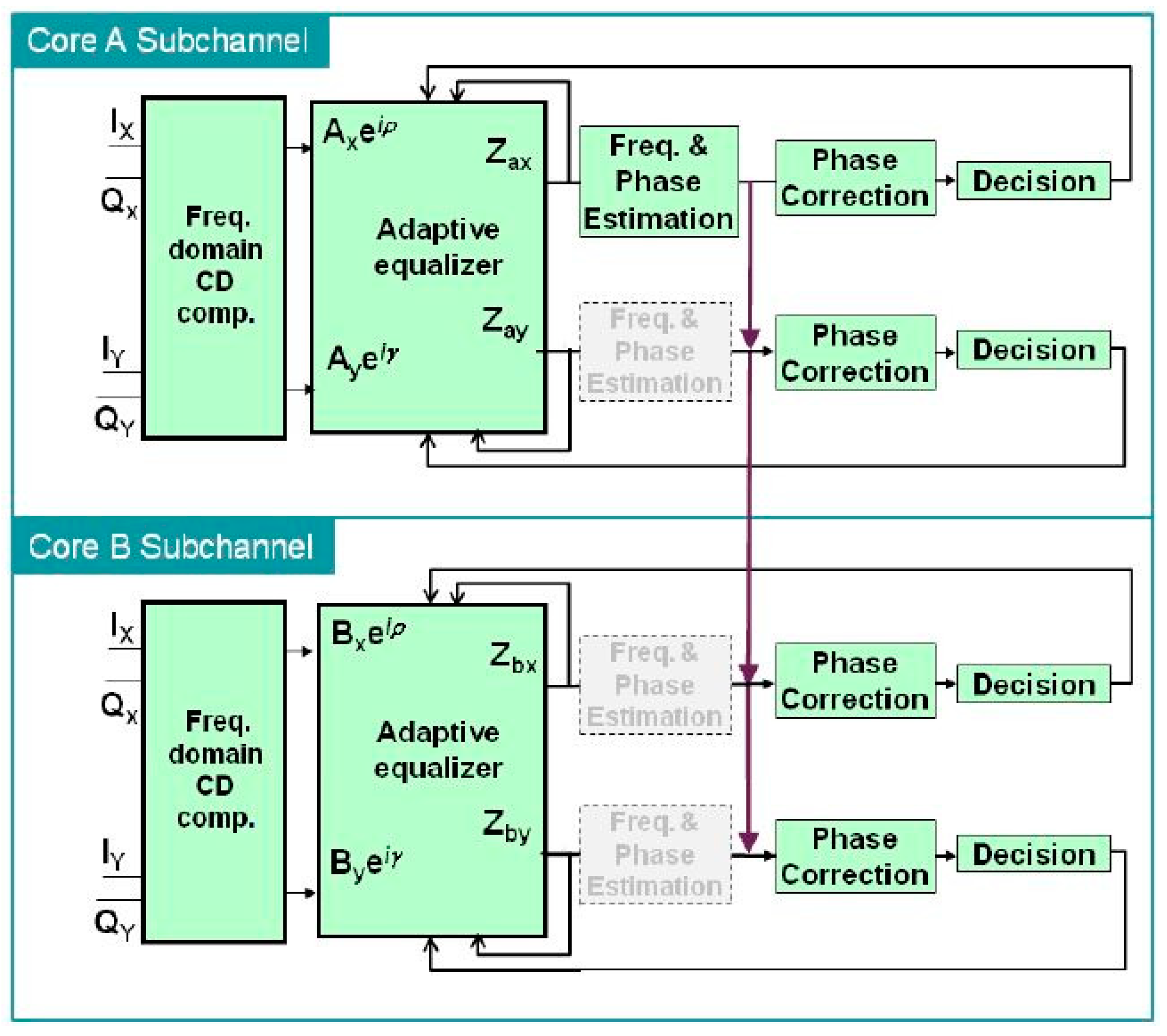
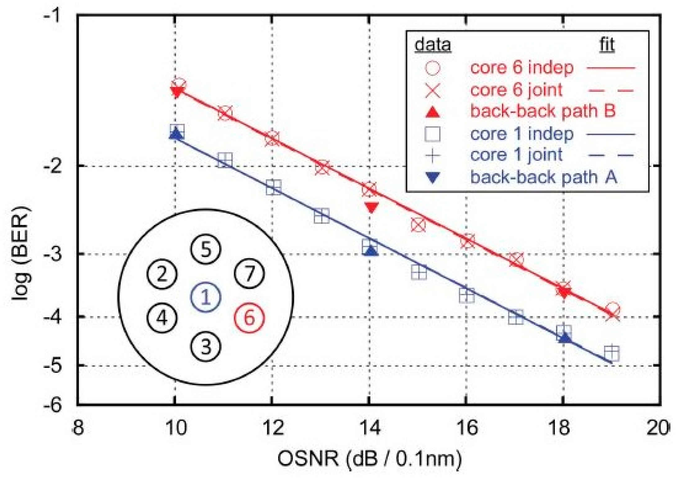
7.3. Joint DSP for MCF-Based SDM

Last but not least, this subsection focuses on a joint DSP scheme for the MCF-based SDM transmission system to reduce the overall cost and power consumption of integrated receivers. There is a strong correlation between the phase fluctuations of the different sub-channels, and the master–slave phase recovery causes no BER degradation. The block diagram of a joint DSP method for an MCF-based SDM transmission system with master–slave phase recovery is presented in Figure 30, which utilizes the phase recovered from a single “master” sub-channel to eradicate phase recovery blocks in the “slave” sub-channels, thus decreasing the overall DSP burden at the receiver side [44].

In addition, the BER versus OSNR observed for master–slave phase recovery using the joint DSP scheme for MCF-based SDM transmission system is presented in Figure 31, which is equivalent to that found with independent phase recovery [45].

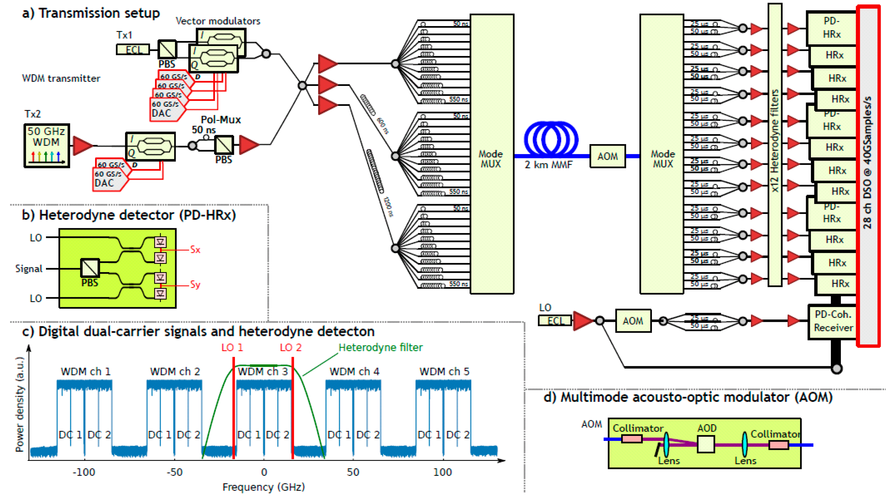
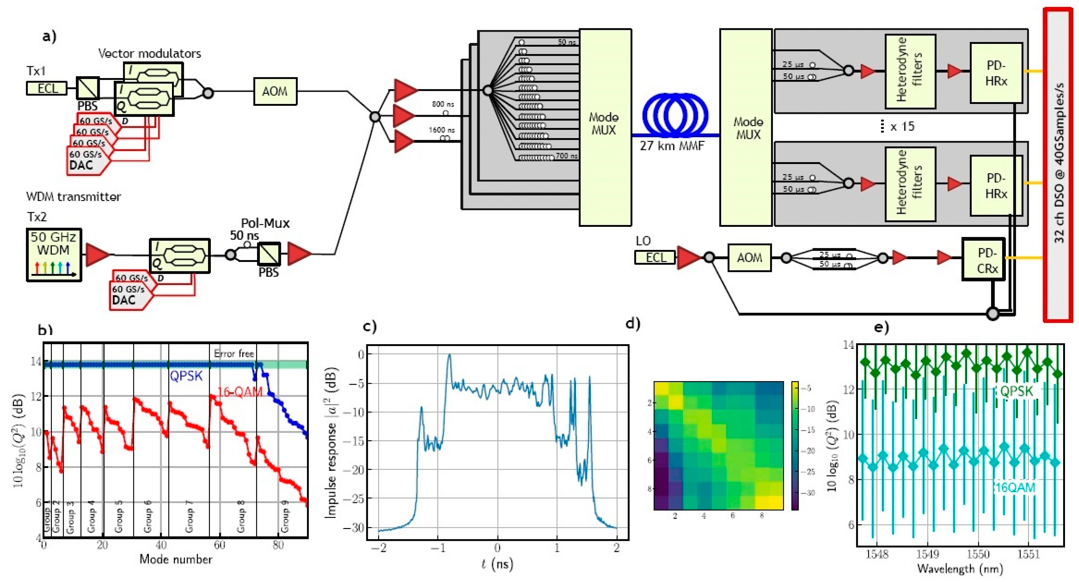
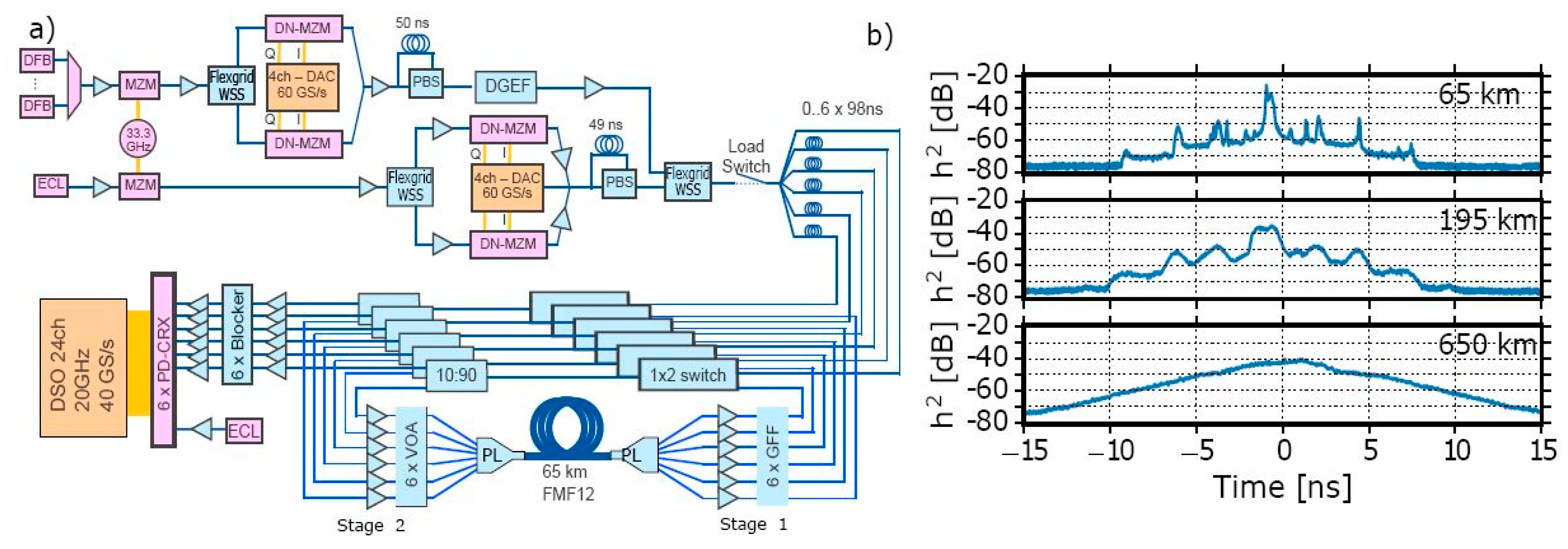
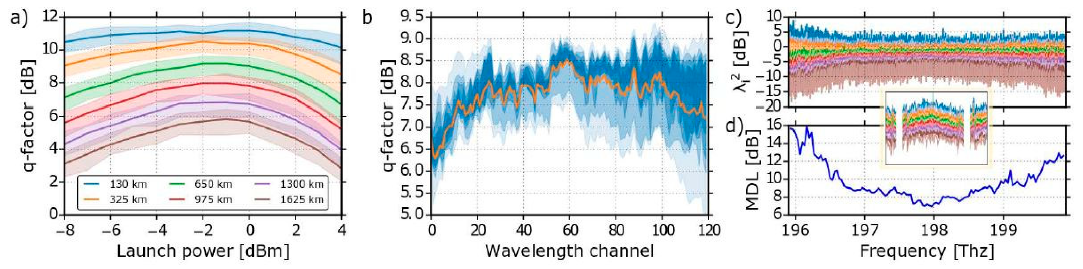
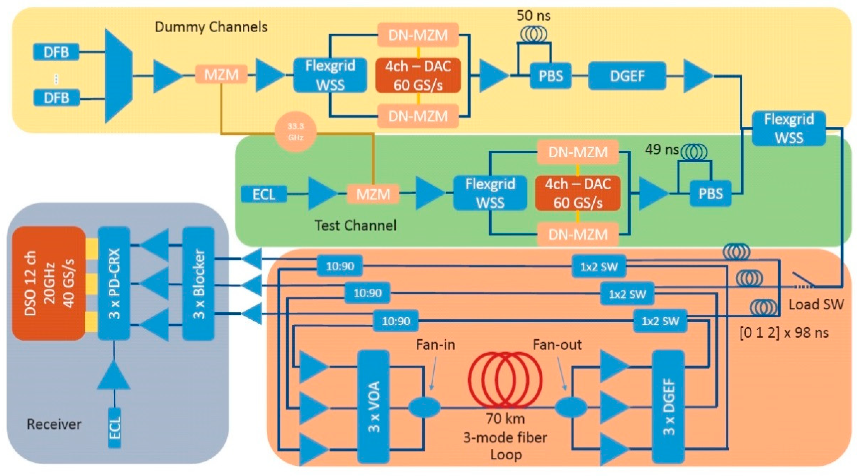
8. Recent Experiments of SDM Transmission Using FMFs

Last but not least, a couple of topical experimental verifications are assessed facilitating a higher transmission capacity for short, medium, and long distances in this section, utilizing FMFs and/or MCFs, along with the progressive maturity of the SDM amplifier, spatial mode coupler, and digital MIMO equalizers to safeguard higher capacity and spectral efficiency.

For instance, Ryf et al. conducted an experiment in 2018 for a MIMO-based 36-mode (two polarization modes) transmission over a 2-km-long 50-μm graded-index multimode fiber (MMF) with a spectral efficiency of 72 bit/s/Hz, as denoted in Figure 32 along with the close-ups of the heterodyne receiver arrangement and multimode acousto-optic modulator, as well as the spectrum of the test signal and location of the heterodyne filters and local oscillator [46]. The results were attained using a 72 × 72 coherent MIMO-DSP, with five 15-Gbaud dual-carrier PDM-QPSK signals with a channel spacing of 50 GHz transmitted.

Figure 33 denotes the experimental set-up of an MIMO-based 45-mode (two polarization modes) MDM transmission over a 26.5-km-long 50-μm graded-index MMF over 20 wavelength channels resulting in a total capacity of 101 Tb/s and a spectral efficiency of 202/bit/s/Hz. The received 90-degree complex amplitude signals were processed by a 90 × 90 MIMO-FDE with 300 symbol-spaced taps, whereas the initial convergence of the equalizer was obtained using the data-aided FD-LMS algorithm with CMA used after that. Then, the carrier-phase recovery and BER counting were performed, while the Q-factors were computed by evaluating an inverse Q function of the BER [47]. The corresponding plots also include the Q-factors of 90 spatial tributaries for QPSK and 16QAM transmission in line with the mode groups, sorted by the performance within the mode group in Figure 33b, with the intensity-averaged impulse response attained from channel estimation over the MMF in Figure 33c, and the intensity transfer matrix showing the coupling between the mode groups in Figure 33d, along with the average Q-factor for QPSK and 16QAM as a function of wavelength in Figure 33e. The error bars within the plots signify the best and the worst spatial tributaries.

In another example, a 138 Tbit/s coherent transmission over six spatial modes plus two polarizations, and 120 wavelength channels carrying 120 Gbit/s mapped 16QAM signals over a 65 $\mathrm{km}$ FMF12 fiber are shown in Figure 34, where low insertion and MDL mode-selective photonic lanterns are used along with a coherent 12 × 12 MIMO equalization using a data-aided FD-LMS algorithm for resolving the modal mixing [48]. The FMF12 fiber is a special FMF designed to have low attenuation for the first 12 spatial channels, while having sufficiently high losses for the higher-order modes to guarantee an effective cut-off. At the receiver side, optical front-end impairment, CD, and frequency-offset compensation is performed, while the carrier phase recovery is performed before calculating performance metrics over 8 million bits per spatial channel. Moreover, the Q-factors versus the launch power averaged for 15 WDM channels, as well as for 120 WDM channels after 650-km transmission are shown in Figure 35, where the gradient of the shaded areas epitomizes the variation in WDM channel performance [48]. In addition, the larger performance variations on the edges of the spectrum, and the singular values for each WDM channel averaged, corresponding to the measured MDL, are depicted in Figure 35c,d, respectively.

Last but not least, the set-up of another 6 × 6 MIMO-based SDM/WDM transmission system using a 70-km DGD-compensated three-mode fiber is shown in Figure 36, whereas the received signals are off-line processed by firstly re-sampling the signals to two samples per signal, along with CD and frequency-offset compensation, which is then followed by a 6 × 6 MIMO FDE with 600 symbol-spaced taps using a data-aided LMS algorithm along with carrier-phase recovery and BER counting for Q-factor calculations [49]. The Q-factors of the center channel at 1550 nm for 64QAM, 16QAM, and QPSK signals as a function of distance for full space-division multiplexed, quasi-single-mode, and single-mode fiber transmission, respectively, are presented in Figure 37, with the markers indicating the measured distances [50]. A summary of these recent experimental validations using MIMO DSP is presented in

Table 2. Summary table of recent experimental validations using multi-input multi-output (MIMO) digital signal processing (DSP). MMF—multimode fiber; FMF—few-mode fiber; MCF—multicore fiber.

Transmission Distance	Spectral Efficiency	DSP Approach	Fiber Type	Number of Modes	Year	Reference
2 km	72 bit/s/Hz	72 × 72 MIMO	50 μm MMF	36 × 2	2018	[46]
26.5 km	202 bit/s/Hz	90 × 90 MIMO	50 μm MMF	45 × 2	2018	[47]
65 km	34.91 bit/s/Hz	12 × 12 MIMO	FMF12	6 × 2	2017	[48]
70 km	9 bit/s/Hz	6 × 6 MIMO	FMF	3 × 2	2017	[49]
9.8 km	947 bit/s/Hz	6 × 6 MIMO	FMF + MCF	3 × 2	2016	[51]
23.8 km	43.63 bit/s/Hz	30 × 30 MIMO	FMF9	15 × 2	2015	[52]
53.7 km	217.6 bit/s/Hz	6 × 6 MIMO	MCF	3 × 2	2016	[53]

while an updated graph of mode numbers versus the transmission distance is presented in Figure 38, which summarizes the state-of-the-art SDM-WDM experiments [51,52,53]. Further improvement in the near future will most likely come from the soft-output maximum-likelihood algorithms, including repeated tree search and single tree search, to further improve the efficiency of the MIMO DSP [54].

9. Conclusions

In this review paper, we presented an overview regarding the state-of-the-art adaptive MIMO equalization for high-speed MDM coherent receivers, including the LMS and RLS techniques, as well as the STBC-assisted RLS algorithms. The performance analysis of various adaptive filtering schemes was presented for QPSK, 16QAM, and 64QAM, along with the STBC-based enhancement amongst different modulation formats. Last but not least, the complexity optimization using the single-stage architecture of CD and DMGD joint compensation was discussed, for reducing the total DSP implementation complexity. Additionally, a number of recent experimental validations were assessed, enabling higher transmission capacity and spectral efficiency for different transmission distances by means of various MIMO DSP approaches.

References

1. Winzer, P.J. Making spatial multiplexing a reality. Nat. Photonics 2014, 8, 345–348. [Google Scholar] [CrossRef]
2. Li, A.; Chen, X.; Amin, A.A.; Ye, J.; Shieh, W. Space-division multiplexed high-speed superchannel transmission over few-mode fiber. J. Lightw. Technol. 2012, 30, 3953–3964. [Google Scholar] [CrossRef]
3. Richardson, D.J.; Fini, J.M.; Nelson, L.E. Space-division multiplexing in optical fibres. Nat. Photonics 2013, 7, 354–362. [Google Scholar] [CrossRef] [Green Version]
4. Ip, E. Recent advances in mode-division multiplexed transmission using few-mode fibers. In Proceedings of the Twenty-Third National Conference on Communications (NCC), Chennai, India, 2–4 March 2017. [Google Scholar]
5. Zhang, Z.; Guo, C.; Cui, L.; Mo, Q.; Zhao, N.; Du, C.; Li, X.; Li, G. 21 spatial mode erbium-doped fiber amplifier for mode division multiplexing transmission. Opt. Lett. 2018, 43, 1550–1553. [Google Scholar] [CrossRef] [PubMed]
6. Jain, S.; Rancaño, V.J.F.; May-Smith, T.C.; Petropoulos, P.; Sahu, J.K.; Richardson, D.J. Multi-element fiber technology for space-division multiplexing applications. Opt. Express 2014, 22, 3787–3796. [Google Scholar] [CrossRef] [PubMed]
7. Pan, Z.; Weng, Y.; He, X.; Wang, J. Adaptive frequency-domain equalization and MIMO signal processing in mode division multiplexing systems using few-mode fibers. In Proceedings of the Signal Processing in Photonic Communications 2016 (SPPCom)—SpW2G.1, Vancouver, BC, Canada, 18–20 July 2016. [Google Scholar]
8. Arık, S.Ö.; Askarov, D.; Kahn, J.M. Adaptive frequency-domain equalization in mode-division multiplexing systems. Opt. Express 2014, 32, 1841–1852. [Google Scholar] [CrossRef]
9. Faruk, M.S.; Kikuchi, K. Adaptive frequency-domain equalization in digital coherent optical receivers. Opt. Express 2011, 19, 12789–12798. [Google Scholar] [CrossRef] [PubMed]
10. Weng, Y.; He, X.; Pan, Z. Performance analysis of low-complexity adaptive frequency-domain equalization and MIMO signal processing for compensation of differential mode group delay in mode-division multiplexing communication systems using few-mode fibers. In Proceedings of the SPIE 9774, Next-Generation Optical Communication: Components, Sub-Systems, and Systems V, 97740B, San Francisco, CA, USA, 13 February 2016. [Google Scholar]
11. Zhu, C.; Tran, A.V.; Do, C.C.; Chen, S.; Anderson, T.; Skafidas, E. Digital signal processing for training-aided coherent optical single-carrier frequency-domain equalization systems. J. Lightw. Technol. 2014, 32, 4110–4120. [Google Scholar]
12. Pittalà, F.; Slim, I.; Mezghani, A.; Nossek, J.A. Training-aided frequency-domain channel estimation and equalization for single-carrier coherent optical transmission systems. J. Lightw. Technol. 2014, 32, 4247–4261. [Google Scholar] [CrossRef]
13. He, X.; Weng, Y.; Wang, J.; Pan, Z. Noise power directed adaptive frequency domain least mean square algorithm with fast convergence for DMGD compensation in few-mode fiber transmission systems. In Proceedings of the Optical Fiber Communication Conference (OFC)—Th3E.1, San Francisco, CA, USA, 9–13 March 2014. [Google Scholar]
14. Puttnam, B.J.; Sakaguchi, J.; Mendinueta, J.M.D.; Klaus, W.; Awaji, Y.; Wada, N.; Kanno, A.; Kawanishi, T. Investigating self-homodyne coherent detection in a 19 channel space-division-multiplexed transmission link. Opt. Express 2013, 21, 1561–1566. [Google Scholar] [CrossRef]
15. Weng, Y.; Wang, T.; Pan, Z. Fast-convergent adaptive frequency-domain recursive least-squares algorithm with reduced complexity for MDM transmission systems using optical few-mode fibers. In Proceedings of the Conference on Lasers and Electro-Optics (CLEO)—SW4F.6, San Jose, CA, USA, 5–10 June 2016. [Google Scholar]
16. Ryf, R.; Weerdenburg, J.V.; Alvarez-Aguirre, R.A.; Fontaine, N.K.; Essiambre, R.-J.; Chen, H.; Alvarado-Zacarias, J.C.; Amezcua-Correa, R.; Koonen, T.; Okonkwo, C. White Gaussian noise based capacity estimate and characterization of fiber-optic links. In Proceedings of the Optical Fiber Communication Conference (OFC)—W1G.2, San Diego, CA, USA, 11–15 March 2018. [Google Scholar]
17. Choutagunta, K.; Arik, S.Ö.; Ho, K.-P.; Kahn, J.M. Characterizing mode-dependent loss and gain in multimode components. J. Lightw. Technol. 2018, 36, 3815–3823. [Google Scholar] [CrossRef]
18. Andrusier, A.; Meron, E.; Feder, M.; Shtaif, M. Optical implementation of a space-time-trellis code for enhancing the tolerance of systems to polarization-dependent loss. Opt. Lett. 2013, 38, 118–120. [Google Scholar] [CrossRef]
19. Mizuno, T.; Takara, H.; Shibahara, K.; Sano, A.; Miyamoto, Y. Dense space division multiplexed transmission over multicore and multimode fiber for long-haul transport systems. J. Lightw. Technol. 2016, 34, 1484–1493. [Google Scholar] [CrossRef]
20. Ip, E.; Milione, G.; Li, M.-J.; Cvijetic, N.; Kanonakis, K.; Stone, J.; Peng, G.; Prieto, X.; Montero, C.; Moreno, V.; Liñares, J. SDM transmission of real-time 10GbE traffic using commercial SFP + transceivers over 0.5 km elliptical-core few-mode fiber. Opt. Express 2015, 23, 17120–17126. [Google Scholar] [CrossRef] [PubMed]
21. Pan, Z.; He, X.; Weng, Y. Hardware efficient frequency domain equalization in few-mode fiber coherent transmission systems. In Proceedings of the SPIE 9009, Next-Generation Optical Communication: Components, Sub-Systems, and Systems III, San Francisco, CA, USA, 1 February 2014. [Google Scholar]
22. Ferreira, F.; Jansen, S.; Monteiro, P.; Silva, H. Nonlinear semi-analytical model for simulation of few-mode fiber transmission. IEEE Photonics Technol. Lett. 2012, 24, 240–242. [Google Scholar] [CrossRef]
23. Poletti, F.; Horak, P. Description of ultrashort pulse propagation in multimode optical fibers. J. Opt. Soc. Am. B 2008, 25, 1645–1654. [Google Scholar] [CrossRef]
24. Mumtaz, S.; Essiambre, R.J.; Agrawal, G.P. Nonlinear propagation in multimode and multicore fibers: Generalization of the manakov equations. J. Lightw. Technol. 2013, 31, 398–406. [Google Scholar] [CrossRef]
25. Ryf, R.; Randel, S.; Gnauck, A.H.; Bolle, C.; Sierra, A.; Mumtaz, S.; Esmaeelpour, M.; Burrows, E.C.; Essiambre, R.-J.; Winzer, P.J.; et al. Mode-division multiplexing over 96 km of few-mode fiber using coherent 6 × 6 MIMO processing. J. Lightw. Technol. 2012, 30, 521–531. [Google Scholar] [CrossRef]
26. Carpenter, J.; Wilkinson, T.D. Mode Division Multiplexing over 2 km of OM2 fibre using rotationally optimized mode excitation with fibre coupler demultiplexer. In Proceedings of the IEEE Photonics Society Summer Topical Meeting Series, Seattle, WA, USA, 9–11 July 2012. [Google Scholar]
27. Weng, Y.; He, X.; Yao, W.; Pacheco, M.; Wang, J.; Pan, Z. Investigation of adaptive filtering and MDL mitigation based on space-time block-coding for spatial division multiplexed coherent receivers. Opt. Fiber Technol. 2017, 36, 231–236. [Google Scholar] [CrossRef]
28. Winzer, P.J.; Foschini, G.J. MIMO capacities and outage probabilities in spatially multiplexed optical transport systems. Opt. Express 2011, 19, 16680–16696. [Google Scholar] [CrossRef] [PubMed]
29. Weng, Y.; He, X.; Yao, W.; Pacheco, M.C.; Wang, J.; Pan, Z. Mode-dependent loss mitigation scheme for PDM-64QAM few-mode fiber space-division-multiplexing systems via STBC-MIMO equalizer. In Proceedings of the Conference on Lasers and Electro-Optics (CLEO), San Jose, CA, USA, 14–19 May 2017. [Google Scholar]
30. Raptis, N.; Grivas, E.; Pikasis, E.; Syvridis, D. Space-time block code based MIMO encoding for large core step index plastic optical fiber transmission systems. Opt. Express 2011, 19, 10336–10350. [Google Scholar] [CrossRef] [PubMed]
31. Weng, Y.; He, X.; Wang, J.; Pan, Z. Rigorous study of low-complexity adaptive space-time block-coded MIMO receivers in high-speed mode multiplexed fiber-optic transmission links using few-mode fibers. In Proceedings of the SPIE 10130, Next-Generation Optical Communication: Components, Sub-Systems, and Systems VI, San Francisco, CA, USA, 28 January 2017. [Google Scholar]
32. Mizusawa, Y.; Kitamura, I.; Kumamoto, K.; Zhou, H. Proposal analysis and basic experimental evaluation of MIMO radio over fiber relay system. In Proceedings of the SPIE 10559, Broadband Access Communication Technologies XII, San Francisco, CA, USA, 29 January 2018. [Google Scholar]
33. He, X.; Weng, Y.; Pan, Z. Fast convergent frequency-domain MIMO equalizer for few-mode fiber communication systems. Opt. Comm. 2018, 409, 131–136. [Google Scholar] [CrossRef]
34. Li, G. Recent advances in coherent optical communication. Adv. Opt. Photonics 2009, 1, 279–307. [Google Scholar] [CrossRef]
35. Muga, N.J.; Fernandes, G.M.; Ziaie, S.; Ferreira, R.M.; Shahpari, A.; Teixeira, A.L.; Pinto, A.N. Advanced digital signal processing techniques based on Stokes space analysis for high-capacity coherent optical systems. In Proceedings of the 19th International Conference on Transparent Optical Networks (ICTON 2017), Girona, Spain, 2–6 July 2017. [Google Scholar]
36. Lin, C.; Djordjevic, I.B.; Zou, D. Achievable information rates calculation for optical OFDM few-mode fiber long-haul transmission systems. Opt. Express 2015, 23, 16846–16856. [Google Scholar] [CrossRef] [PubMed]
37. Inan, B.; Jansen, S.L.; Spinnler, B.; Ferreira, F.; Borne, D.V.D.; Kuschnerov, M.; Lobato, A.; Adhikari, S.; Sleiffer, V.A.; Hanik, N. DSP requirements for MIMO spatial multiplexed receivers. In Proceedings of the IEEE Photonics Society Summer Topical Meeting Series, Seattle, WA, USA, 9–11 July 2012. [Google Scholar]
38. Pan, Z.; He, X.; Weng, Y. Frequency domain equalizer in few-mode fiber space-division-multiplexing systems. In Proceedings of the 23rd Wireless and Optical Communication Conference (WOCC), Newark, NJ, USA, 9–10 May 2014. [Google Scholar]
39. Dick, C.; Amiri, K.; Cavallaro, J.R.; Rao, R. Design and architecture of spatial multiplexing MIMO decoders for FPGAs. In Proceedings of the 42nd Asilomar Conference on Signals, Systems and Computers, Pacific Grove, CA, USA, 26–29 October 2008. [Google Scholar]
40. Cvijetic, N.; Ip, E.; Prasad, N.; Li, M.J.; Wang, T. Experimental time and frequency domain MIMO channel matrix characterization versus distance for 6 × 28 Gbaud QPSK transmission over 40 × 25 km few mode fiber. In Proceedings of the Optical Fiber Communication Conference (OFC), San Francisco, CA, USA, 9–13 March 2014. [Google Scholar]
41. Awwad, E.; Othman, G.R.; Jaouën, Y. Space-time coding and optimal scrambling for mode multiplexed optical fiber systems. In Proceedings of the IEEE International Conference on Communications (ICC), London, UK, 8–12 June 2015. [Google Scholar]
42. Salsi, M.; Koebele, C.; Sperti, D.; Tran, P.; Mardoyan, H.; Brindel, P.; Bigo, S.; Boutin, A.; Verluise, F.; Sillard, P.; et al. Mode-Division Multiplexing of 2 × 100 Gb/s Channels Using an LCOS-Based Spatial Modulator. J. Lightw. Technol. 2012, 30, 618–623. [Google Scholar] [CrossRef]
43. Weng, Y.; He, X.; Pan, Z. Space division multiplexing optical communication using few-mode fibers. Opt. Fiber Technol. 2017, 36, 155–180. [Google Scholar] [CrossRef]
44. Feuer, M.D.; Nelson, L.E.; Zhou, X.; Woodward, S.L.; Isaac, R.; Zhu, B.; Taunay, T.F.; Fishteyn, M.; Fini, J.F.; Yan, M.F. Demonstration of joint DSP receivers for spatial superchannels. In Proceedings of the IEEE Photonics Society Summer Topical Meeting Series, Seattle, WA, USA, 9–11 July 2012. [Google Scholar]
45. Feuer, M.D.; Nelson, L.E.; Zhou, X.; Woodward, S.L.; Isaac, R.; Zhu, B.; Taunay, T.F.; Fishteyn, M.; Fini, J.F.; Yan, M.F. Joint digital signal processing receivers for spatial superchannels. IEEE Photonics Technol. Lett. 2012, 24, 1957–1960. [Google Scholar] [CrossRef]
46. Ryf, R.; Fontaine, N.K.; Chen, H.; Wittek, S.; Li, J.; Alvarado-Zacarias, J.C.; Amezcua-Correa, R.; Antonio-Lopez, J.E.; Capuzzo, M.; Kopf, R.; et al. Mode-multiplexed transmission over 36 spatial modes of a graded-index multimode fiber. In Proceedings of the European Conference on Optical Communication (ECOC), Rome, Italy, 23–27 September 2018. [Google Scholar]
47. Ryf, R.; Fontaine, N.K.; Wittek, S.; Choutagunta, K.; Mazur, M.; Chen, H.; Alvarado-Zacarias, J.C.; Amezcua-Correa, R.; Capuzzo, M.; Kopf, R.; et al. High-spectral-efficiency mode-multiplexed transmission over graded-index multimode fiber. In Proceedings of the European Conference on Optical Communication (ECOC), Rome, Italy, 23–27 September 2018. [Google Scholar]
48. Weerdenburg, J.V.; Ryf, R.; Alvarado-Zacarias, J.C.; Alvarez-Aguirre, R.A.; Fontaine, N.K.; Chen, H.; Amezcua-Correa, R.; Koonen, T.; Okonkwo, C. 138 Tbit/s transmission over 650 km graded-index 6-mode fiber. In Proceedings of the European Conference on Optical Communication (ECOC), Gothenburg, Sweden, 17–21 September 2017. [Google Scholar]
49. Rademacher, G.; Ryf, R.; Fontaine, N.K.; Chen, H.; Essiambre, R.-J.; Puttnam, B.J.; Luis, R.S.; Awaji, Y.; Wada, N.; Gross, S.; et al. 3500-km mode-multiplexed transmission through a three-mode graded-index few-mode fiber link. In Proceedings of the European Conference on Optical Communication (ECOC), Gothenburg, Sweden, 17–21 September 2017. [Google Scholar]
50. Rademacher, G.; Ryf, R.; Fontaine, N.K.; Chen, H.; Essiambre, R.-J.; Puttnam, B.J.; Luis, R.S.; Awaji, Y.; Wada, N.; Gross, S.; et al. Long-Haul Transmission Over Few-Mode Fibers with Space-Division Multiplexing. J. Lightw. Technol. 2018, 36, 1382–1388. [Google Scholar] [CrossRef]
51. Igarashi, K.; Soma, D.; Wakayama, Y.; Takeshima, K.; Kawaguchi, Y.; Yoshikane, N.; Tsuritani, T.; Morita, I.; Suzuki, M. Ultra-dense spatial-division-multiplexed optical fiber transmission over 6-mode 19-core fibers. Opt. Express 2016, 24, 10213–10231. [Google Scholar] [CrossRef]
52. Fontaine, N.K.; Ryf, R.; Chen, H.; Velazquez Benitez, A.; Antonio Lopez, J.E.; Amezcua Correa, R.; Guan, B.; Ercan, B.; Scott, R.P.; Yoo, S.J.B.; et al. 30 × 30 MIMO Transmission over 15 Spatial Modes. In Proceedings of the Optical Fiber Communication Conference (OFC), Los Angeles, CA, USA, 22–26 March 2015. [Google Scholar]
53. Luís, R.S.; Rademacher, G.; Puttnam, B.J.; Awaji, Y.; Wada, N. Long distance crosstalk-supported transmission using homogeneous multicore fibers and SDM-MIMO demultiplexing. Opt. Express 2018, 26, 24044–24053. [Google Scholar] [CrossRef]
54. Garcia-Moll, V.M.; Simarro, M.A.; Martínez-Zaldívar, F.J.; González, A.; Vidala, A.M. Maximum likelihood soft-output detection through Sphere Decoding combined with box optimization. Signal Process. 2016, 125, 249–260. [Google Scholar] [CrossRef]
Figure 1. The typical examples of optical fibers for space division multiplexing (SDM) technology: (a) multi-element fiber; (b) multicore fiber; (c) multi-mode fiber [4].
Applsci 09 01178 g001
Figure 2. The recent records of spatial multiplicity vs. the transmission distance in the state-of-the-art SDM-WDM experiments [19].
Applsci 09 01178 g002
Figure 3. The typical coherent receiver configuration for a single-carrier transmission system with a 6 × 6 multi-input multi-output (MIMO) frequency-domain equalization (FDE) [7].
Applsci 09 01178 g003
Figure 4. The squared magnitude of the 6 × 6 impulse responses for MIMO equalization [25].
Applsci 09 01178 g004
Figure 5. Eye diagrams of a typical mode-division multiplexing (MDM) transmission system for (a) back-to-back; (b) over-fill launch without coupler; (c) LP01 channel; (d) LP12 channel [26].
Applsci 09 01178 g005
Figure 6. Schematic of an MDM system utilizing the MIMO FDE [31].
Applsci 09 01178 g006
Figure 7. The space and time allocation for the space–time block-coding (STBC)-aided recursive least squares (RLS) algorithm [31].
Applsci 09 01178 g007
Figure 8. The architecture of an STBC-aided RLS equalizer for MDM receivers [29].
Applsci 09 01178 g008
Figure 9. Block diagram of the digital signal processing (DSP) subsystems of a coherent transceiver using a Stokes space-based polarization de-multiplexing (PolDemux) algorithm [35].
Applsci 09 01178 g009
Figure 10. The orthogonal frequency-division multiplexing (OFDM) FDE equalizer complexity requirements compared with other MIMO approaches [37].
Applsci 09 01178 g010
Figure 11. A scalable architecture of spatial multiplexing MIMO decoders for field-programmable gate arrays (FPGAs) [39].
Applsci 09 01178 g011
Figure 12. Configuration of a six-mode coherent transmission system [29].
Applsci 09 01178 g012
Figure 13. The normalized mean square error (NMSE) vs. the number of fast Fourier transform (FFT) blocks for various algorithms for a polarization-division multiplexing (PDM) quadrature phase shift keying (QPSK) signal; inset: constellation diagrams before (right) and after (left) the STBC-RLS compensation [27].
Applsci 09 01178 g013
Figure 14. The NMSE vs. the number of FFT blocks for various algorithms for a PDM 16 quadrature amplitude modulation (16QAM) signal; inset: constellation diagrams before (right) and after (left) the STBC-RLS compensation [27].
Applsci 09 01178 g014
Figure 15. The NMSE vs. the number of FFT blocks for various algorithms for a PDM-64QAM signal; inset: constellation diagrams before (right) and after (left) the STBC-RLS compensation [27].
Applsci 09 01178 g015
Figure 16. The bit error rate (BER) vs. optical signal-to-noise ratio (OSNR) comparison for PDM-QPSK signal in LP11a mode with or without using the STBC-RLS scheme [31].
Applsci 09 01178 g016
Figure 17. The BER vs. OSNR comparison for PDM-16QAM signal in LP11a mode with or without using the STBC-RLS scheme [31].
Applsci 09 01178 g017
Figure 18. The BER vs. OSNR comparison for PDM-64QAM signal in LP11a mode with or without using the STBC-RLS scheme [31].
Applsci 09 01178 g018
Figure 19. The summary of BER vs. OSNR for various modulation formats with or without using STBC-RLS compensation [29].
Applsci 09 01178 g019
Figure 20. Mode-dependent loss (MDL) probability distribution functions under different coupling levels [41].
Applsci 09 01178 g020
Figure 21. The BER vs. OSNR for three different modes for a PDM-QPSK signal using the STBC-RLS scheme [27].
Applsci 09 01178 g021
Figure 22. The BER vs. OSNR for three different modes for a PDM-16QAM signal using the STBC-RLS scheme [27].
Applsci 09 01178 g022
Figure 23. The BER vs. OSNR for three different modes for a PDM-64QAM signal using the STBC-RLS scheme [27].
Applsci 09 01178 g023
Figure 24. The finite impulse response (FIR) filter illustration, along with Q2-factor vs. tap number for both 2 × 2 and 4 × 4 MIMO cases [42].
Applsci 09 01178 g024
Figure 25. The number of taps per carrier for MIMO DSP vs. distance in recent few-mode fiber (FMF) transmission experiments [19].
Applsci 09 01178 g025
Figure 26. The representation of a coherent receiver with the joint compensation of chromatic dispersion (CD) plus differential mode group delay (DMGD) through a single-stage MIMO architecture [10].
Applsci 09 01178 g026
Figure 27. The required complex multiplications per output symbol of the two-stage and single-stage frequency-domain (FD)-RLS approaches as a function of transmission distance in an FMF-based transmission system [10].
Applsci 09 01178 g027
Figure 28. The Q-value vs. step size using both two-stage and single-stage FD-RLS algorithms as a function of transmission distance in an FMF-based transmission system [15].
Applsci 09 01178 g028
Figure 29. The convergence speed comparison of two FD-LMS algorithms and single-stage FD-RLS algorithms at different OSNRs [7].
Applsci 09 01178 g029
Figure 30. A joint DSP approach for multicore fiber (MCF)-based SDM transmission system with master–slave phase recovery [44].
Applsci 09 01178 g030
Figure 31. BER vs. OSNR for MCF-based SDM transmission system using the joint DSP scheme [45].
Applsci 09 01178 g031
Figure 32. (a) Setup of a 72 × 72 MIMO-based transmission; (b) heterodyne receiver arrangement; (c) spectrum of the test signal and location of the heterodyne filters and local oscillator; (d) multimode acousto-optic modulator [46].
Applsci 09 01178 g032
Figure 33. (a) Setup of a 90 × 90 MIMO-based transmission; (b) Q-factors for QPSK and 16QAM; (c) intensity-averaged impulse response attained; (d) intensity transfer matrix; (e) average Q-factor for QPSK and 16QAM [47].
Applsci 09 01178 g033
Figure 34. (a) Set-up of a 12 × 12 MIMO-based transmission; (b) impulse response after 65-, 195-, and 650-km transmission [48].
Applsci 09 01178 g034
Figure 35. (a) Q-factors vs. power for 15 WDM channels; (b) Q-factors vs. WDM channels; (c) singular values after 650-km transmission; (d) average MDL vs. frequency per WDM channel [48].
Applsci 09 01178 g035
Figure 36. Setup of a 6 × 6 MIMO-based transmission [49].
Applsci 09 01178 g036
Figure 37. Q-factors for 64QAM, 16QAM, and QPSK [50].
Applsci 09 01178 g037
Figure 38. Updated graph of mode numbers vs. the transmission distance in the state-of-the-art SDM-WDM experiments.
Applsci 09 01178 g038