On the Coherence Relationship between Measurement Matrices and Equivalent Radiation Sources in Microwave Computational Imaging Applications

Abstract

In recent years, computational imaging, which encodes scene information into a set of measurements, has become a research focus in the field of microwave imaging. As with other typical inverse problems, the key challenge is to reduce the mutual coherences in the measurement matrix which is composed of measurement modes. Since the modes are synthesized by antennas, there is a great deal of interest in the antenna optimization for the reduction. The mechanism underlying the generation of the coherences is critical for the optimization; however, relevant research is still inadequate. In this paper, we try to address the research gap by relating the coherences to the antennas’ equivalent radiation sources via spectral Green’s dyad. We demonstrate that the coherences in the measurement matrix are dependent on the spatial spectral coherences of the sources, while in this relationship the imaging scenario acts as a spectral low-pass filter. Increasing the imaging range narrows the spectral constraint, which eventually increases the coherences in the measurement matrix. Full-wave electromagnetic simulations are performed for validation. We hope that our work provides a possible direction for the antenna optimization in microwave computational imaging (MCI) applications and motivates further research in this field.

1. Introduction

As a new paradigm first proposed in the mid-1990s, computational imaging transfers the burden of image formation from solely optical physics to both front-end measurements and post-detection processing, providing a desired imaging capability with reduced requirements in size, weight, power or cost [1]. A key feature of this paradigm is indirect measurements of probed objects, as opposed to direct ones in conventional approaches. Inspired by this feature, MCI illuminates the object with incoherent measurement modes, encoding spatial information into multiple measurements. Given the forward radiation model, the object is then retrieved from the echoes by post processing. Essentially, MCI transfers the complexity of microwave imaging systems from hardware to modelling and algorithms, thus enabling huge flexibility in modalities and avoiding the dependence on mechanical movements and antenna apertures that are densely populated with complex electronic components. In recent years, the emergence of electromagnetic metamaterials, which possesses unprecedented ability in the control of electromagnetic fields and thus greatly caters for the need of generating incoherent modes, has immensely promoted relevant research on MCI and made this paradigm one of the most popular topics in the field of microwave imaging [2,3,4,5].

Mathematically, MCI solves a nonlinear Fredholm integral equation of the first kind, which belongs to a typical category of inverse problems [6]. In discrete form, the integral equation can be rewritten as a matrix equation in which the measurement modes in the measurements composes a measurement matrix. According to Reference [7], the integral (i.e., the measurement matrix) functions as a transformation from the space of the object, to the measurement space which is spanned by independent measurement modes. The imaging of the object, that is, the inverse of the transformation, naturally possesses nonlinear, ill-posed and instable characteristics, making it difficult to reconstruct from the echoes in the presence of noise [6,8]. In order to ameliorate these ill conditions, it is crucial to enlarge the number of effective bases. In addition, some researchers demonstrated that the square of the spatial resolution is usually equal to the ratio of the image area to the number of independent modes [7]. The aim of enlarging the number of independent bases necessitates the minimization of the mutual coherences in the measurement matrix. Since the measurement modes are synthesized by antennas, the antenna optimization for the coherence minimization has become a research focus.

According to Reference [9], in order to reduce the mutual coherences, an interesting option is to construct the modes as independent and identically distributed as random variables. Thus various antenna structures have been proposed for MCI by intuitively randomizing resonant cavity structures or element resonant properties, such as mode-mixing cavity [10], printed aperiodic cavity with irises distributed in a Fibonacci pattern [11], disordered cavity with dynamically tuneable impedance source [12] and printed metasurface with subwavelength metallic cylinders in the cavity [13]. These antennas have shown that the mutual coherences in the measurement matrix can be effectively reduced by introducing disorder and randomness in the antenna structures. However, these heuristic works do not give an explicit formulation of the coherences’ formation, which burdens further theoretical analysis and optimization. For the antenna apertures assembled by elements with random resonant frequencies, it has been widely examined that the increase of the elements’ quality factors leads to the decreases in both the coherences and radiation efficiency [14,15]. However, this superficial phenomenon is still far from an explicit explanation of the mechanism underlying the generation of the coherences. In Reference [16], the researchers proposed a spatial spectral analysis on the coverage of the Ewald sphere and obtained a convolutional relationship between the transmitting and receiving antennas on the sphere. The analysis in spectral domain (k-space) is very illuminating because it gives an intuitive and approximate approach of evaluating the imaging performance of MCI systems. However, the authors did not formulate the coherences in the frame of the k-space analysis. Recently, some researchers achieved average mutual coherence minimization of the measurement matrix in a two-dimensional (2D) planar imaging scenario [17]. In that work, the minimization is implemented using augmented Lagrangian method, while the positions of the antennas serve as the optimization variables. Despite the impressive results, the formation of the coherences is not investigated and the imaging scenario in which the antennas fully surround the region of interest (ROI) may not be applicable for many microwave imaging applications where the angle of view (AOV) is limited. Overall, the research gap between the mutual coherences in the measurement matrix and the antennas needs to be addressed by rigorous electromagnetic analysis. However, to the best of our knowledge, relevant research is still inadequate.

Apart from microwave imaging, in the fields of optics and wireless communication, the researches on electromagnetic degree of freedom (EM DOF) may shed light on the investigation of the mutual coherences. In inverse problems, the EM DOF indicates the maximum amount of information that can be retrieved from echoes in the presence of noise [18]. For an imaging system, the number of EM DOF can be associated with the number of the system’s effective eigenvalues that suffice for reconstruction and thus in negative relationship with the mutual coherences of the measurements. According to Reference [19], the number of EM DOF is strongly dependent on the geometry of imaging scenario and will saturate to a upper-bound due to the presence of noise when continuously expanding the transmit or receive volumes. In Reference [20], the researchers proposed wavevector-aperture-product (WAP) which characterizes the number of EM DOF in a scattering environment, giving a clearer view of the scenario geometry’s influence on the EM DOF. These works on EM DOF imply that the mutual coherences in the measurement matrix may be related to the spatial spectrum of the radiation sources in MCI applications, while the geometry of the imaging scenario constitutes a constraint condition in this relationship.

Inspired by the above works, we relate the mutual coherences in the measurement matrix to the antennas by formulating the electric fields of the antennas’ equivalent sources via spectral Green’s dyad. In our derivation, the antennas are replaced by the equivalent sources with the purpose of simplifying the problem under consideration. These sources can be real, induced or fictitious, that is, sources that appears as a result of electromagnetic equivalence theorem. Our work shows that the mutual coherences are dependent on the spectral coherences of the sources, while the imaging scenario acts equivalently as a low-pass filter in the k-space. Growing the imaging range narrows this spectral constraint and thus leads to surges in the mutual coherences, which is in accordance with previous work in which the number of EM DOF is bounded by the WAP. Full-wave electromagnetic simulations are performed for validation, where a set of spatially modulated magnetic currents and a set of typical cELC apertures are introduced as fictitious and real radiation sources respectively. In the validation, the coherence level of a matrix is evaluated by the average mutual coherence that is calculated between rows and the one that is calculated between columns, respectively.

The rest of this paper is organized as follows. In Section 2, the derivation of the coherence relationship is presented. The full-wave validation is performed in Section 3. Finally, we give the conclusions and future direction in Section 4.

2. Derivation of the Coherence Relationship

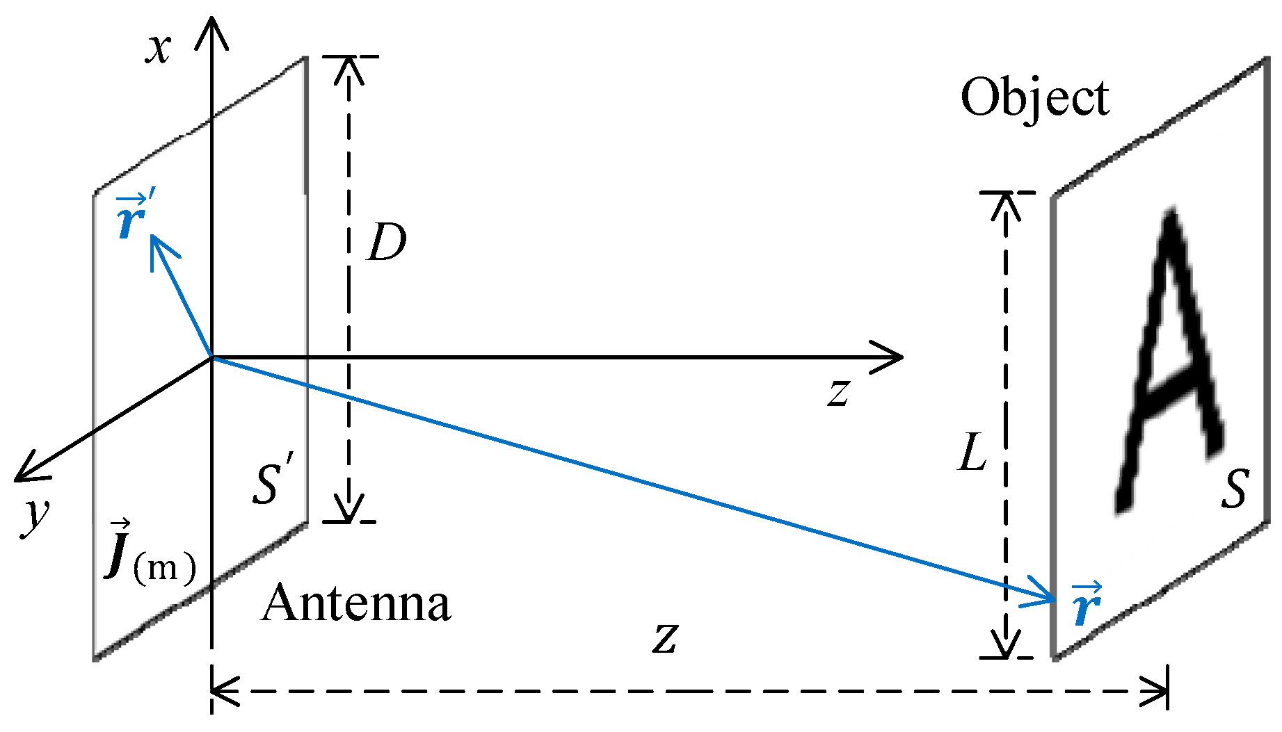
Consider a typical microwave imaging scenario as shown in Figure 1. As in most MCI applications, the AOV of the scenario is finite.

In Figure 1, $S^{\prime }$ and $S$ denote the antenna volumes and the ROI respectively. According to electromagnetic equivalence theorem, the antennas are replaced by equivalent electric current density $\overrightarrow{\mathit{J}}$ or magnetic current density ${\overrightarrow{\mathit{J}}}_{\mathrm{m}}$ (i.e., equivalent radiation sources). Utilizing 2D spectral Green’s dyad, we can formulate the electric fields in the corresponding 2D k-space [21]:

$$\begin{gathered} \widetilde{\overrightarrow{\mathit{E}}}({\overrightarrow{\mathit{k}}}_{xy},z)=-\frac{k_0{Z}_0{\mathrm{e}}^{\mathrm{j}{k}_{z}z}}{2k_z}(\overleftrightarrow{\mathbf{I}}-\widehat{\mathit{k}}\widehat{\mathit{k}})·\widetilde{\overrightarrow{\mathit{J}}} \\ \widetilde{\overrightarrow{\mathit{E}}}({\overrightarrow{\mathit{k}}}_{xy},z)=\frac{k_0{\mathrm{e}}^{\mathrm{j}{k}_{z}z}}{2k_z}\widehat{\mathit{k}}\times {\widetilde{\overrightarrow{\mathit{J}}}}_{\mathrm{m}} \end{gathered}$$

(1)

where $\overleftrightarrow{\mathbf{I}}$ is the unit dyad, $Z_0$ and $k_0$ are the wave impedance and the spatial frequency in free space, $\widehat{\mathit{k}}$ denotes the unit vector of the wave vector $\overrightarrow{\mathit{k}}$ and $k_z=\sqrt{k_0^2-k_{xy}^2}$. Equation (1) shows that the transverse spatial frequency $k_{xy}$ in the propagational components of the fields is bounded by $k_0$ because of the presence of ${\mathrm{e}}^{\mathrm{j}{k}_{z}z}$.

Transforming the fields radiated by $\widetilde{\overrightarrow{\mathit{J}}}$ in Equation (1) into spatial domain gives:

$$\overrightarrow{\mathit{E}}\left({\overrightarrow{\mathit{r}}}_{xy},z\right)=-\frac{k_0{Z}_0}{4\mathsf{\pi }}{\int }_{-\infty }^{\infty }\frac{(\overleftrightarrow{\mathbf{I}}-\widehat{\mathit{k}}\widehat{\mathit{k}})·\widetilde{\overrightarrow{\mathit{J}}}}{k_z}{\mathrm{e}}^{\mathrm{j}\overrightarrow{\mathit{k}}·\overrightarrow{\mathit{r}}}{\mathrm{d}}^2{\overrightarrow{\mathit{k}}}_{xy}$$

(2)

According to Reference [22], the integral in Equation (2) can be solved by stationary phase approximation because $\overrightarrow{\mathit{k}}·\overrightarrow{\mathit{r}}$ is stationary at the critical points distruibuting in the ROI. Define $\phi =\overrightarrow{\mathit{k}}·\overrightarrow{\mathit{r}}$, then it gives the gradient vector ${\nabla }_{{\overrightarrow{\mathit{k}}}_{xy}}\phi$ and Hessian matrix $\mathbf{Hess}$ as:

$$\begin{gathered} {\nabla }_{{\overrightarrow{\mathit{k}}}_{xy}}\phi ={[\begin{array}{cc}x-k_{x}z/k_z& y-k_{y}z/k_z\end{array}]}^{\mathrm{T}} \\ \mathbf{Hess}=-\frac{z}{k_z^3}\left[\begin{array}{cc}{k}_x^2+k_z^2& k_x{k}_y\\ k_x{k}_y& k_y^2+k_z^2\end{array}\right] \end{gathered}$$

(3)

Equation (3) shows that the critical points ${\overrightarrow{\mathit{k}}}_{xy}^{*}$ are give by ${[\begin{array}{cc}{k}_{0}x/r& k_{0}y/r\end{array}]}^{\mathrm{T}}$ where x and y vary in the ROI. These points correspond to the positions in the ROI where particular plane-wave components are illuminated [22]. According to Reference [23], at the critical points, Equation (2) integrates to:

$$\begin{array}{ll}\overrightarrow{\mathit{E}}({\overrightarrow{\mathit{r}}}_{xy},z)& \approx -\frac{k_0{Z}_0}{4\mathsf{\pi }}\left\{{\mathrm{e}}^{\mathrm{j}\phi ({\overrightarrow{\mathit{k}}}_{xy}^{*})}{|\det [\mathbf{Hess}({\overrightarrow{\mathit{k}}}_{xy}^{*})]|}^{-\frac{1}{2}}{\mathrm{e}}^{\mathrm{j}\frac{\mathsf{\pi }}{4}\mathrm{sign}[\mathrm{Hess}({\overrightarrow{\mathit{k}}}_{xy}^{*})]}2\mathsf{\pi }{\left[\frac{(\overleftrightarrow{\mathbf{I}}-\widehat{\mathit{k}}\widehat{\mathit{k}})·\widetilde{\overrightarrow{\mathit{J}}}}{k_z}\right]}_{{\overrightarrow{\mathit{k}}}_{xy}^{*}}+o\left(\frac{1}{k_0}\right)\right\}\\ & \approx -\frac{k_0{Z}_0}{2r}{\mathrm{e}}^{\mathrm{j}(k_{0}r-\frac{\mathsf{\pi }}{4})}{\left[(\overleftrightarrow{\mathbf{I}}-\widehat{\mathit{k}}\widehat{\mathit{k}})·\widetilde{\overrightarrow{\mathit{J}}}\right]}_{{\overrightarrow{\mathit{k}}}_{xy}^{*}}\end{array}$$

(4)

Similarly, by the same procedures, the fields radiated by ${\overrightarrow{\mathit{J}}}_{\mathrm{m}}$ can be obtained:

$$\overrightarrow{\mathit{E}}\left({\overrightarrow{\mathit{r}}}_{xy},z\right)\approx \frac{k_0}{2r}{\mathrm{e}}^{\mathrm{j}\left(k_{0}r-\frac{\mathsf{\pi }}{4}\right)}{\left(\widehat{\mathit{k}}\times {\widetilde{\overrightarrow{\mathit{J}}}}_{\mathrm{m}}\right)}_{{\overrightarrow{\mathit{k}}}_{xy}^{*}}$$

(5)

Equations (4) and (5) formulate $\overrightarrow{\mathit{E}}$ radiated by $\overrightarrow{\mathit{J}}$ and ${\overrightarrow{\mathit{J}}}_{\mathrm{m}}$ respectivley in the 2D k-space.

Before we proceed, it is necessary to investigate the influence of the scenario geometry on the spatial spectrum of the fields in the ROI. In order to formulate the spectrum, we define a window function $w\left({\overrightarrow{\mathit{r}}}_{xy}\right)$ in the ROI:

$$w\left({\overrightarrow{\mathit{r}}}_{xy}\right)=\{\begin{array}{c}1, {\overrightarrow{\mathit{r}}}_{xy}\in S\\ 0, {\overrightarrow{\mathit{r}}}_{xy}\notin S\end{array}$$

(6)

Implementing inverse Fourier transformation to Equation (5) with (6) yields:

$${\widetilde{\overrightarrow{\mathit{E}}}}_w\left({\overrightarrow{\mathit{k}}}_{xy},z\right)={\int }_{-\infty }^{\infty }\left(w\overrightarrow{\mathit{E}}\right){\mathrm{e}}^{-\mathrm{j}{\overrightarrow{\mathit{k}}}_{xy}·{\overrightarrow{\mathit{r}}}_{xy}}{\mathrm{d}}^2{\overrightarrow{\mathit{r}}}_{xy}$$

(7)

By the similar procedures implemented previously, applying stationary phase approximation to Equation (7) gives the amplitude of the spectrum:

$$\begin{gathered} |{\widetilde{\overrightarrow{\mathit{E}}}}_w({\overrightarrow{\mathit{k}}}_{xy},z)|\approx \mathsf{\pi }{Z}_0|(\overleftrightarrow{\mathbf{I}}-\widehat{\mathit{k}}\widehat{\mathit{k}})·\widetilde{\overrightarrow{\mathit{J}}}|w({\overrightarrow{\mathit{r}}}_{xy}^{*}) \\ |{\widetilde{\overrightarrow{\mathit{E}}}}_w({\overrightarrow{\mathit{k}}}_{xy},z)|\approx \mathsf{\pi }|\widehat{\mathit{k}}\times {\widetilde{\overrightarrow{\mathit{J}}}}_{\mathrm{m}}|w({\overrightarrow{\mathit{r}}}_{xy}^{*}) \end{gathered}$$

(8)

where the critical points ${\overrightarrow{\mathit{r}}}_{xy}^{*}$ distruibuting in the 2D k-space are given by:

$${\overrightarrow{\mathit{r}}}_{xy}^{*}=\left[\begin{array}{c}{k}_x\sqrt{\frac{k_y^2{x}^2+k_0^2{z}^2}{\left(k_0^2-k_x^2\right)\left(k_0^2-k_y^2\right)}}\\ k_y\sqrt{\frac{k_x^2{y}^2+k_0^2{z}^2}{\left(k_0^2-k_x^2\right)\left(k_0^2-k_y^2\right)}}\end{array}\right]$$

(9)

It shows that the spectrum is bounded in the k-space due to the presence of $w\left({\overrightarrow{\mathit{r}}}_{xy}^{*}\right)$. With the purpose of simplifying the imaging scenario under consideration, the ROI is set to a square with the size of L at the imaging range of z (Figure 1). Thus combining Equation (6) with (9) gives an approximation of the cut-off spatial frequency of the spectrum:

$$|k_{x,y}|\le k_{0}L/2z$$

(10)

Equation (10) shows that the scenario geometry functions equivalently as a low-pass filter in the k-space of which the cut-off frequency varies with the AOV of the ROI. The filter shrinks with the increasing of the imaging range. Therefore, the spectrum of the fields in the ROI are bounded in a low-pass area (denoted as LPF for convenience) in the k-space due to not only the propagational components but also the finite AOV of the imaging scenario.

In the next, the coherence relationship will be discussed. Before the discussion, we briefly introduce the electromagnetic model for MCI. In this model, the echo signals are formulated by the measurement mode h sampling the contrast function x of the object:

$$\begin{gathered} g={\int }_{S}hx{\mathrm{d}}^2\overrightarrow{\mathit{r}} \\ h=-\frac{\mathrm{j}{k}_0}{Z_0}\overrightarrow{\mathit{E}}·{\overrightarrow{\mathit{E}}}_{\mathrm{Rx}} \\ x={\tilde{\epsilon }}_{\mathrm{r}}-1={\epsilon }_{\mathrm{r}}-\mathrm{j}\sigma /\omega {\epsilon }_0-1 \end{gathered}$$

(11)

where $g$ is the echo, ${\epsilon }_{\mathrm{r}}$ and $\sigma$ are the relative permittivity and the conductivity of the object respectively, $\overrightarrow{\mathit{E}}$ is the field generated by the incident field ${\overrightarrow{\mathit{E}}}_{\mathrm{Tx}}$ illuminating the object and ${\overrightarrow{\mathit{E}}}_{\mathrm{Rx}}$ is the field radiated by the receiving antennas with normalized excitation [24]. Comparing with the model used for electromagnetic inverse scattering imaging [23]:

$$\begin{gathered} {\overrightarrow{\mathit{E}}}_{\mathrm{sca}}={\int }_S\overleftrightarrow{\mathit{G}}·\mathrm{O}\overrightarrow{\mathit{E}}{\mathrm{d}}^2\overrightarrow{\mathit{r}} \\ \mathrm{O}=k_0^2\left({\tilde{\epsilon }}_{\mathrm{r}}-1\right) \end{gathered}$$

(12)

where $\mathrm{O}$ is the same quantity as $x$ omitting the constant $k_0^2$, $\overleftrightarrow{\mathit{G}}$ is dyadic Green’s function in free space and ${\overrightarrow{\mathit{E}}}_{\mathrm{sca}}$ is the scattering field, it shows that Equation (12) does not consider the generation of the echo. When the generation is considered, the measurement mode h, which is the dot production $\overrightarrow{\mathit{E}}·{\overrightarrow{\mathit{E}}}_{\mathrm{Rx}}$, appears in the integral as a result of electromagnetic reciprocity:

$$g\propto {\int }_{S^{\prime }}{\overrightarrow{\mathit{E}}}_{\mathrm{inc}}·{\overrightarrow{\mathit{J}}}_{\mathrm{Rx}}{\mathrm{d}}^2{\overrightarrow{\mathit{r}}}^{\prime }={\int }_{S^{\prime }}{\int }_S\overleftrightarrow{\mathit{G}}·\mathrm{O}\overrightarrow{\mathit{E}}{\mathrm{d}}^2\overrightarrow{\mathit{r}}·{\overrightarrow{\mathit{J}}}_{\mathrm{Rx}}{\mathrm{d}}^2{\overrightarrow{\mathit{r}}}^{\prime }\propto {\int }_{S}x\left(\overrightarrow{\mathit{E}}·{\overrightarrow{\mathit{E}}}_{\mathrm{Rx}}\right){\mathrm{d}}^2\overrightarrow{\mathit{r}}$$

(13)

where ${\overrightarrow{\mathit{E}}}_{\mathrm{inc}}$ is ${\overrightarrow{\mathit{E}}}_{\mathrm{sca}}$ at the receiving antenna region $S^{\prime }$ and ${\overrightarrow{\mathit{J}}}_{\mathrm{Rx}}$ is the virtual electric current density that generates ${\overrightarrow{\mathit{E}}}_{\mathrm{Rx}}$. Essentially, Equation (11) is obtained by the combination of Equation (12) and the reciprocity of the receiving antennas, while the scattering of the receiving antennas is omitted. A detailed derivation of Equation (11) can be found in Reference [5,24].

As shown in Equation (13), the object can be deemed as a secondary radiation source which is stimulated by $\overrightarrow{\mathit{E}}$ illuminating the object. Unfortunately, $\overrightarrow{\mathit{E}}$ is dependent on not only the incident field ${\overrightarrow{\mathit{E}}}_{\mathrm{Tx}}$ but also the object itself, making the imaging model a nonlinear problem. To settle the nonlinearity, researchers have proposed many iterative approaches, such as Born iterative method [6]. However, in most MCI applications, the interaction can be neglected by applying Born approximation without obviously deteriorating the imaging quality due to the short wavelength of microwaves (the applicability of Born approximation is another big issue that seems to go beyond the scope of this paper; relevant detailed discussion can be found in Reference [23]). Therefore, Born approximation, which ignores the perturbation of the object and replaces $\overrightarrow{\mathit{E}}$ with ${\overrightarrow{\mathit{E}}}_{\mathrm{Tx}}$, is widely applied in MCI.

Born approximation is also adopted in our analysis. Hence, neither the measurement nor the coherence is affected by the object. Under this approximation, the measurement mode can be formulated by ${\overrightarrow{\mathit{E}}}_{\mathrm{Tx}}$ and ${\overrightarrow{\mathit{E}}}_{\mathrm{Rx}}$:

$$h\left(\overrightarrow{\mathit{r}}\right)=-\frac{\mathrm{j}{k}_0}{Z_0}{\overrightarrow{\mathit{E}}}_{\mathrm{Tx}}\left(\overrightarrow{\mathit{r}}\right)·{\overrightarrow{\mathit{E}}}_{\mathrm{Rx}}\left(\overrightarrow{\mathit{r}}\right)$$

(14)

In discrete form, the model can be represented by a matrix equation: $\mathbf{g}=\mathbf{Hx}$, where $\mathbf{g}$ is an echo vector, $\mathbf{H}={[\begin{array}{ccc}{\mathit{h}}_1^{\mathrm{T}}& \cdots & {\mathit{h}}_M^{\mathrm{T}}\end{array}]}^{\mathrm{T}}$ is the measurement matrix which is composed of the measurement modes in multiple measurements, M and N are the numbers of the measurements and the grid of the ROI respectively and $\mathbf{x}$ is the contrast function of the object.

The matrix $\mathbf{H}$ transforms the space of the object to the measurement space spanned by incoherent measurement modes, encoding the object’s spatial information into the echoes. Hence, the object can be retrieved via the inverse of $\mathbf{H}$. However, this inverse problem always possess natural ill-posedness due to deficient rank of $\mathbf{H}$ and the presence of noise. In practice, the number of effective bases supporting the measurement space is always inadequate to support the space of the object, which leads to inevitable losses of spatial information during the above-mentioned transformation. Thus, it is critical to construct the bases in the measurement space as more as possible, which requires reducing the mutual coherences in $\mathbf{H}$. As $\mathbf{H}$ is generated by the radiations of the equivalent radiation sources, the mutual coherences in $\mathbf{H}$ results from the mutual coherences of the sources.

In order to formulate the relationship between the two sets of mutual coherences, we start with row correlations of the matrix $\widehat{\mathbf{H}}$ which is the matrix $\mathbf{H}$ with ${\ell }_2$ normalized rows. Analogously to Gramian matrix, we define the average mutual coherence ${\mu }^{\mathrm{T}}$ that is calculating in rows and ${[\widehat{\mathbf{H}}{\widehat{\mathbf{H}}}^{*}]}_{ij}$ which is the mutual coherence between measurement #i and #j:

$$\begin{gathered} {\mu }^{\mathrm{T}}\left(\mathbf{H}\right)=\frac{{\sum }_{i\ne j}{|{[\widehat{\mathbf{H}}{\widehat{\mathbf{H}}}^{*}]}_{ij}|}^2}{M\left(M-1\right)} \\ {[\widehat{\mathbf{H}}{\widehat{\mathbf{H}}}^{*}]}_{ij}=⟨h_i\left(\overrightarrow{\mathit{r}}\right),h_j\left(\overrightarrow{\mathit{r}}\right)⟩={\int }_S\frac{h_i\left(\overrightarrow{\mathit{r}}\right)}{\Vert h_i\left(\overrightarrow{\mathit{r}}\right)\Vert }\frac{h_j^{*}\left(\overrightarrow{\mathit{r}}\right)}{\Vert h_j\left(\overrightarrow{\mathit{r}}\right)\Vert }{\mathrm{d}}^2\overrightarrow{\mathit{r}} \end{gathered}$$

(15)

where the superscript * denotes conjugate transpose and $<>$ denotes coherence calculation. The coherence ${\mu }^{\mathrm{T}}$ accumulates from every ${[\widehat{\mathbf{H}}{\widehat{\mathbf{H}}}^{*}]}_{ij}$ and thus provides an indication of the mutual coherence level of the entire matrix $\mathbf{H}$. With the aim of relating the mutual coherence ${[\widehat{\mathbf{H}}{\widehat{\mathbf{H}}}^{*}]}_{ij}$ to the equivalent radiation sources, we substitute Equation (14) into (15), which gives:

$${[\widehat{\mathbf{H}}{\widehat{\mathbf{H}}}^{*}]}_{ij}=\frac{1}{Z_0^2}{⟨k_i{\overrightarrow{\mathit{E}}}_i^{\mathrm{Tx}}\left(\overrightarrow{\mathit{r}}\right)·{\overrightarrow{\mathit{E}}}_i^{\mathrm{Rx}}\left(\overrightarrow{\mathit{r}}\right),k_j{\overrightarrow{\mathit{E}}}_j^{\mathrm{Tx}}\left(\overrightarrow{\mathit{r}}\right)·{\overrightarrow{\mathit{E}}}_j^{\mathrm{Rx}}\left(\overrightarrow{\mathit{r}}\right)⟩}_{\overrightarrow{\mathit{r}}\in S}$$

(16)

where $k_i$ is the spatial frequency in free space in measurement #i. Then substituting Equations (4) and (5) into (16) gives ${[\widehat{\mathbf{H}}{\widehat{\mathbf{H}}}^{*}]}_{ij}$ represented by $\widetilde{\overrightarrow{\mathit{J}}}$ or ${\widetilde{\overrightarrow{\mathit{J}}}}_{\mathrm{m}}$ respectively:

$$\begin{gathered} {[\widehat{\mathbf{H}}{\widehat{\mathbf{H}}}^{*}]}_{ij}=\frac{Z_0^2}{16}{⟨\frac{k_i^3{\mathrm{e}}^{\mathrm{j}2k_{i}r}}{r^2}{\widetilde{\overrightarrow{\mathit{J}}}}_i^{\mathrm{Tx}}·{(\overleftrightarrow{\mathbf{I}}-\widehat{\mathit{k}}\widehat{\mathit{k}})}^2·{\widetilde{\overrightarrow{\mathit{J}}}}_i^{\mathrm{Rx}},\frac{k_j^3{\mathrm{e}}^{\mathrm{j}2k_{j}r}}{r^2}{\widetilde{\overrightarrow{\mathit{J}}}}_j^{\mathrm{Tx}}·{(\overleftrightarrow{\mathbf{I}}-\widehat{\mathit{k}}\widehat{\mathit{k}})}^2·{\widetilde{\overrightarrow{\mathit{J}}}}_j^{\mathrm{Rx}}⟩}_{{\overrightarrow{\mathit{k}}}_{i,j}^{*}=k_{i,j}\overrightarrow{\mathit{r}}/r, \overrightarrow{\mathit{r}}\in S} \\ {[\widehat{\mathbf{H}}{\widehat{\mathbf{H}}}^{*}]}_{ij}=\frac{1}{16Z_0^2}{⟨\frac{k_i^3{\mathrm{e}}^{\mathrm{j}2k_{i}r}}{r^2}{\widetilde{\overrightarrow{\mathit{J}}}}_i^{\mathrm{m},\mathrm{Tx}}·(\overleftrightarrow{\mathbf{I}}-\widehat{\mathit{k}}\widehat{\mathit{k}})·{\widetilde{\overrightarrow{\mathit{J}}}}_i^{\mathrm{m},\mathrm{Rx}},\frac{k_j^3{\mathrm{e}}^{\mathrm{j}2k_{j}r}}{r^2}{\widetilde{\overrightarrow{\mathit{J}}}}_j^{\mathrm{m},\mathrm{Tx}}·(\overleftrightarrow{\mathbf{I}}-\widehat{\mathit{k}}\widehat{\mathit{k}})·{\widetilde{\overrightarrow{\mathit{J}}}}_j^{\mathrm{m},\mathrm{Rx}}⟩}_{{\overrightarrow{\mathit{k}}}_{i,j}^{*}=k_{i,j}\overrightarrow{\mathit{r}}/r, \overrightarrow{\mathit{r}}\in S} \end{gathered}$$

(17)

where ‘m’ in the superscript denotes magnetic currents.

In most microwave imaging scenarios, the AOV is a small angle, which leads to $\overleftrightarrow{\mathbf{I}}-\widehat{\mathit{k}}\widehat{\mathit{k}}\approx \overleftrightarrow{\mathbf{I}}$ and $r\approx z$. Applying these approximations to Equation (17), it is convenient to transform the independent variable of the right-hand-side (RHS) from $\overrightarrow{\mathit{r}}$ to ${\overrightarrow{\mathit{k}}}_{xy}^{*}$. Omitting constant coefficients, the transformed equation with the variable ${\overrightarrow{\mathit{k}}}_{xy}^{*}$ can therefore be formulated within the low-pass area (LPF):

$$\begin{gathered} {[\widehat{\mathbf{H}}{\widehat{\mathbf{H}}}^{*}]}_{ij}\propto {⟨k_i^3{\mathrm{e}}^{\mathrm{j}{\varphi }_i}{\widetilde{\overrightarrow{\mathit{J}}}}_i^{\mathrm{Tx}}·{\widetilde{\overrightarrow{\mathit{J}}}}_i^{\mathrm{Rx}},k_j^3{\mathrm{e}}^{\mathrm{j}{\varphi }_j}{\widetilde{\overrightarrow{\mathit{J}}}}_j^{\mathrm{Tx}}·{\widetilde{\overrightarrow{\mathit{J}}}}_j^{\mathrm{Rx}}⟩}_{\mathrm{LPF}} \\ {[\widehat{\mathbf{H}}{\widehat{\mathbf{H}}}^{*}]}_{ij}\propto {⟨k_i^3{\mathrm{e}}^{\mathrm{j}{\varphi }_i}{\widetilde{\overrightarrow{\mathit{J}}}}_i^{\mathrm{m},\mathrm{Tx}}·{\widetilde{\overrightarrow{\mathit{J}}}}_i^{\mathrm{m},\mathrm{Rx}},k_j^3{\mathrm{e}}^{\mathrm{j}{\varphi }_j}{\widetilde{\overrightarrow{\mathit{J}}}}_j^{\mathrm{m},\mathrm{Tx}}·{\widetilde{\overrightarrow{\mathit{J}}}}_j^{\mathrm{m},\mathrm{Rx}}⟩}_{\mathrm{LPF}} \end{gathered}$$

(18)

where the phase term in Equation (17) is denoted by $\varphi$ for convenience in expression:

$$\varphi =2k_{0}r=2z{k}_0^2/k_z^{*}$$

(19)

Furthermore, if the frequencies of the measurements are bounded in a narrow band, which makes ${\mathrm{e}}^{\mathrm{j}\varphi }$ negligible, an approximate form of Equation (18) can be yielded:

$$\begin{gathered} {[\widehat{\mathbf{H}}{\widehat{\mathbf{H}}}^{*}]}_{ij}\propto {⟨{\widetilde{\overrightarrow{\mathit{J}}}}_i^{\mathrm{Tx}}·{\widetilde{\overrightarrow{\mathit{J}}}}_i^{\mathrm{Rx}},{\widetilde{\overrightarrow{\mathit{J}}}}_j^{\mathrm{Tx}}·{\widetilde{\overrightarrow{\mathit{J}}}}_j^{\mathrm{Rx}}⟩}_{\mathrm{LPF}} \\ {[\widehat{\mathbf{H}}{\widehat{\mathbf{H}}}^{*}]}_{ij}\propto {⟨{\widetilde{\overrightarrow{\mathit{J}}}}_i^{\mathrm{m},\mathrm{Tx}}·{\widetilde{\overrightarrow{\mathit{J}}}}_i^{\mathrm{m},\mathrm{Rx}},{\widetilde{\overrightarrow{\mathit{J}}}}_j^{\mathrm{m},\mathrm{Tx}}·{\widetilde{\overrightarrow{\mathit{J}}}}_j^{\mathrm{m},\mathrm{Rx}}⟩}_{\mathrm{LPF}} \end{gathered}$$

(20)

For convenience in expression, we discretize the RHS of Equation (20) and rewrite it as:

$${[\widehat{\mathbf{H}}{\widehat{\mathbf{H}}}^{*}]}_{ij}\propto {[\widehat{\mathbf{S}}{\widehat{\mathbf{S}}}^{*}]}_{ij}$$

(21)

where the source matrix $\mathbf{S}$ is composed of ${({\widetilde{\overrightarrow{\mathit{J}}}}^{\mathrm{Tx}}·{\widetilde{\overrightarrow{\mathit{J}}}}^{\mathrm{Rx}})}_{\mathrm{LPF}}$ or ${({\widetilde{\overrightarrow{\mathit{J}}}}^{\mathrm{m},\mathrm{Tx}}·{\widetilde{\overrightarrow{\mathit{J}}}}^{\mathrm{m},\mathrm{Rx}})}_{\mathrm{LPF}}$ in discrete form:

$$\begin{gathered} {[\mathbf{S}]}_{ij}={\widetilde{\overrightarrow{\mathit{J}}}}_i^{\mathrm{Tx}}({\overrightarrow{\mathit{k}}}_j)·{\widetilde{\overrightarrow{\mathit{J}}}}_i^{\mathrm{Rx}}({\overrightarrow{\mathit{k}}}_j) \\ {[\mathbf{S}]}_{ij}={\widetilde{\overrightarrow{\mathit{J}}}}_i^{\mathrm{m},\mathrm{Tx}}({\overrightarrow{\mathit{k}}}_j)·{\widetilde{\overrightarrow{\mathit{J}}}}_i^{\mathrm{m},\mathrm{Rx}}({\overrightarrow{\mathit{k}}}_j) \\ {\overrightarrow{\mathit{k}}}_j\in \mathrm{LPF} \end{gathered}$$

(22)

Thus far, the mutual coherences in the measurement matrix are explicitly related to the spectral mutual coherences of the equivalent radiation sources:

$$\widehat{\mathbf{H}}{\widehat{\mathbf{H}}}^{*}\propto \widehat{\mathbf{S}}{\widehat{\mathbf{S}}}^{*}$$

(23)

while in this relationship the imaging scenario functions equivalently as a low-pass filter in the k-space. Equation (21) implies that the bases in the measurement space evolves from the bases of the sources via the ‘lossy’ projections of Green’s function within limited AOV. According to Equation (10), growing the imaging range narrows the constraint in the k-space, which inevitably leads to more ‘losses’ in the projections. This is in accordance with the researches on the EM DOF we introduced in previous section.

3. Full-Wave Validation and Discussion

In this section, we validate the proposed coherence relationship by three numerical full-wave electromagnetic simulations and a commercial full-wave simulation (Ansoft HFSS). The imaging scenario in the simulations is set as shown in Figure 1 with $D=L=300\mathrm{mm}$ while the imaging range varies. During the comparisons in each simulation with varying ranges, other parameters in this simulation remain invariable.

In the numerical simulations, a square which is filled by homogeneous, monochromic ($\lambda =10\mathrm{mm}$) and unitarily polarized magnetic currents is introduced as the equivalent radiation sources of the antenna in the region $S^{\prime }$. For simplification of these simulations, this antenna is used for both transmitting and receiving. Because the sources in Equation (22) are formulated in the k-space, we apply spatial frequency modulations to the source in order to demonstrate the relationship or the low-pass filter or generate enough samples of the sources that are ergodic in the k-space. Different spatial frequency modulations are applied for specific purpose in respective simulation. The electric fields in the ROI are calculated via spatial Green’s dyad:

$$\begin{gathered} \overleftrightarrow{\mathit{G}}\left({\overrightarrow{\mathit{r}}}_i,{\overrightarrow{\mathit{r}}}_j^{\prime }\right)=\frac{{\mathrm{e}}^{\mathrm{j}{k}_0{R}_{ij}}}{4\mathsf{\pi }{R}_{ij}}\left[\left(1+\frac{\mathrm{j}}{k_0{R}_{ij}}-\frac{1}{k_0^2{R}_{ij}^2}\right)\overleftrightarrow{\mathbf{I}}+\left(-1-\frac{\mathrm{j}3}{k_0{R}_{ij}}+\frac{3}{k_0^2{R}_{ij}^2}\right){\widehat{\mathit{R}}}_{ij}{\widehat{\mathit{R}}}_{ij}\right] \\ {\overleftrightarrow{\mathit{G}}}_{\mathrm{m}}\left({\overrightarrow{\mathit{r}}}_i,{\overrightarrow{\mathit{r}}}_j^{\prime }\right)=\nabla \times \overleftrightarrow{\mathit{G}}\left({\overrightarrow{\mathit{r}}}_i,{\overrightarrow{\mathit{r}}}_j^{\prime }\right) \end{gathered}$$

(24)

The matrix $\mathbf{H}$ is generated by the inner productions of the electric fields according to Equation (14).

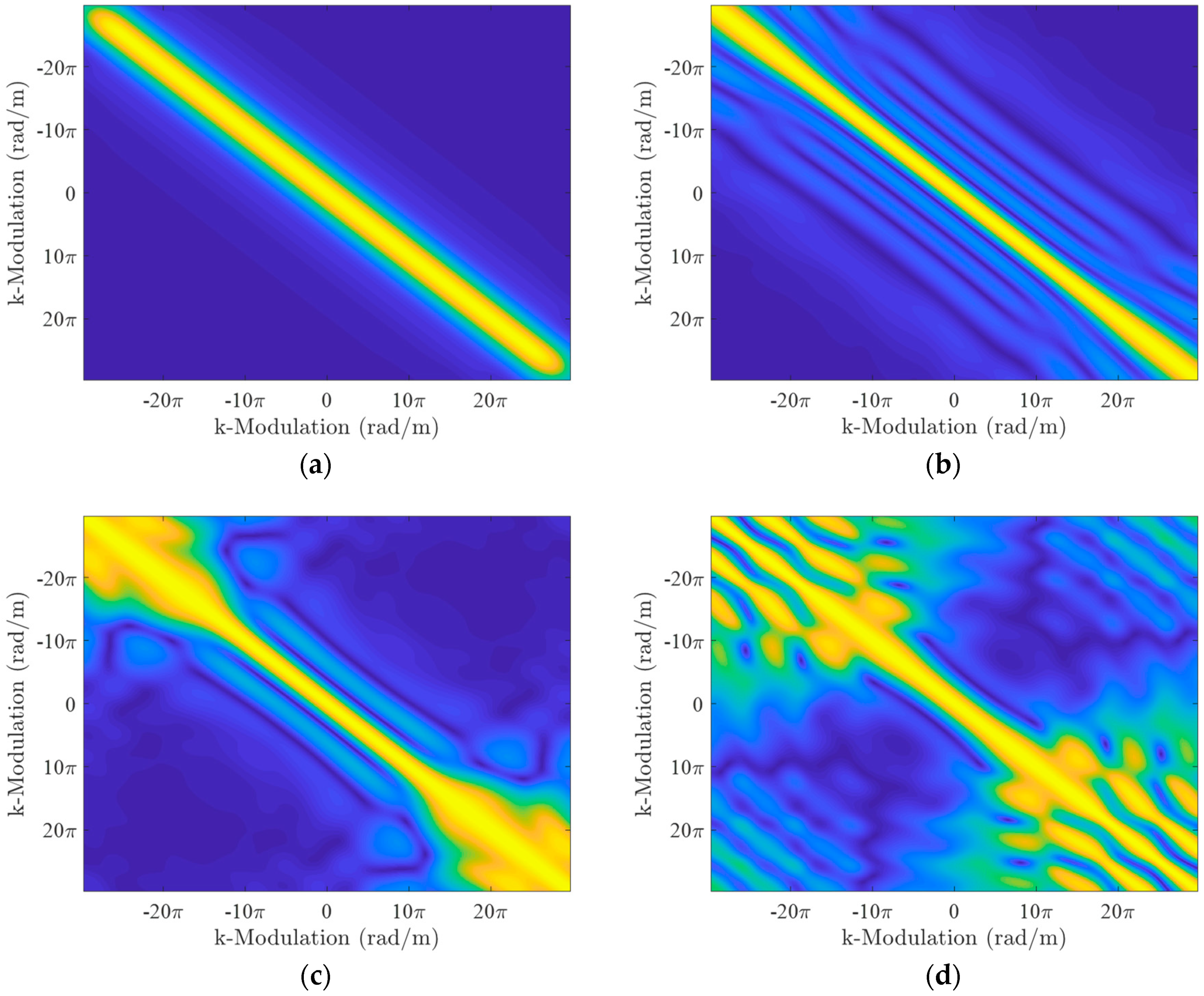
Firstly, we start with the validation of the low-pass filter in the k-space by the first numerical simulation. For explicit demonstration, the source is simultaneously modulated by a set of spatial frequencies. These spatial frequencies are uniformly distributed in the low-pass area in the k-space at the imaging range of 1 m (see Equation (10)). Then implementing Fourier transformation to the source and the measurement modes gives a demonstration of the low-pass filter:

In Figure 2, the spatial spectrum of the modulated source is shown in (a), where each spectrum with respective modulation frequencies can be evidently distinguished. The spectra of the measurement modes at the imaging range of 1 m, 2 m and 4 m are shown in (b), (c) and (d) respectively. By comparison, it shows that the components with high spatial frequency are substantially attenuated with the increasing of the imaging range, which approximately conforms to Equation (10). This result validates that the imaging scenario acts equivalently as a spectral low-pass filter of which the cut-off frequency decreases with the increasing of the imaging range.

In order to demonstrate the coherence properties of the measurement modes and the source, we perform the second numerical simulation in which the modulation of the source is changed. In this simulation, the source is modulated by a spatial frequency that is linearly increased from $-30\mathsf{\pi }$ to $30\mathsf{\pi }$ rad/m, while the directions of these frequencies are identical. In each measurement, only one modulation frequency is applied. According to Fourier analysis, the spectral coherence of the source can be reduced by applying the spatial modulation that shifts its spatial spectrum. If the proposed coherence relationship (i.e., Equation (20)) is valid, the mutual coherence between the measurement modes would decrease with the increasing of the distance between the spatial modulation frequencies applied to the source. Therefore, we observe and compare the amplitudes of the spectral coherence of the source (i.e., matrix $\widehat{\mathbf{S}}{\widehat{\mathbf{S}}}^{*}$) and the mutual coherence of the measurement modes (i.e., matrix $\widehat{\mathbf{H}}{\widehat{\mathbf{H}}}^{*}$). The results are shown in Figure 3, where (a) is the amplitude of $\widehat{\mathbf{S}}{\widehat{\mathbf{S}}}^{*}$, (b–d) are of the respective $\widehat{\mathbf{H}}{\widehat{\mathbf{H}}}^{*}$ at the imaging range of 1 m, 2 m and 4 m.

Figure 3 shows that the most energy of $\widehat{\mathbf{S}}{\widehat{\mathbf{S}}}^{*}$ concentrates on the main diagonal, implying that only the measurement modes with adjacent modulation frequencies are coherent. This phenomenon proves that the spectral coherences of the source is reduced by the spatial modulation that avoids spectrum overlapping. With the linear spatial frequency modulation, the source possesses ideal coherence property. $\widehat{\mathbf{H}}{\widehat{\mathbf{H}}}^{*}$ at different imaging ranges resembles to $\widehat{\mathbf{S}}{\widehat{\mathbf{S}}}^{*}$, while side lobes appear symmetrically along the main diagonal. There are significant upsurges in the mutual coherences of the measurement modes with high spatial frequency modulation when the imaging range is increased. The result suggests that the mutual coherences in the measurement matrix is dependent on the spectral coherences of the sources, while the high spatial frequency components’ attenuation that is imposed by shrinking low-pass area in the k-space increases the coherences.

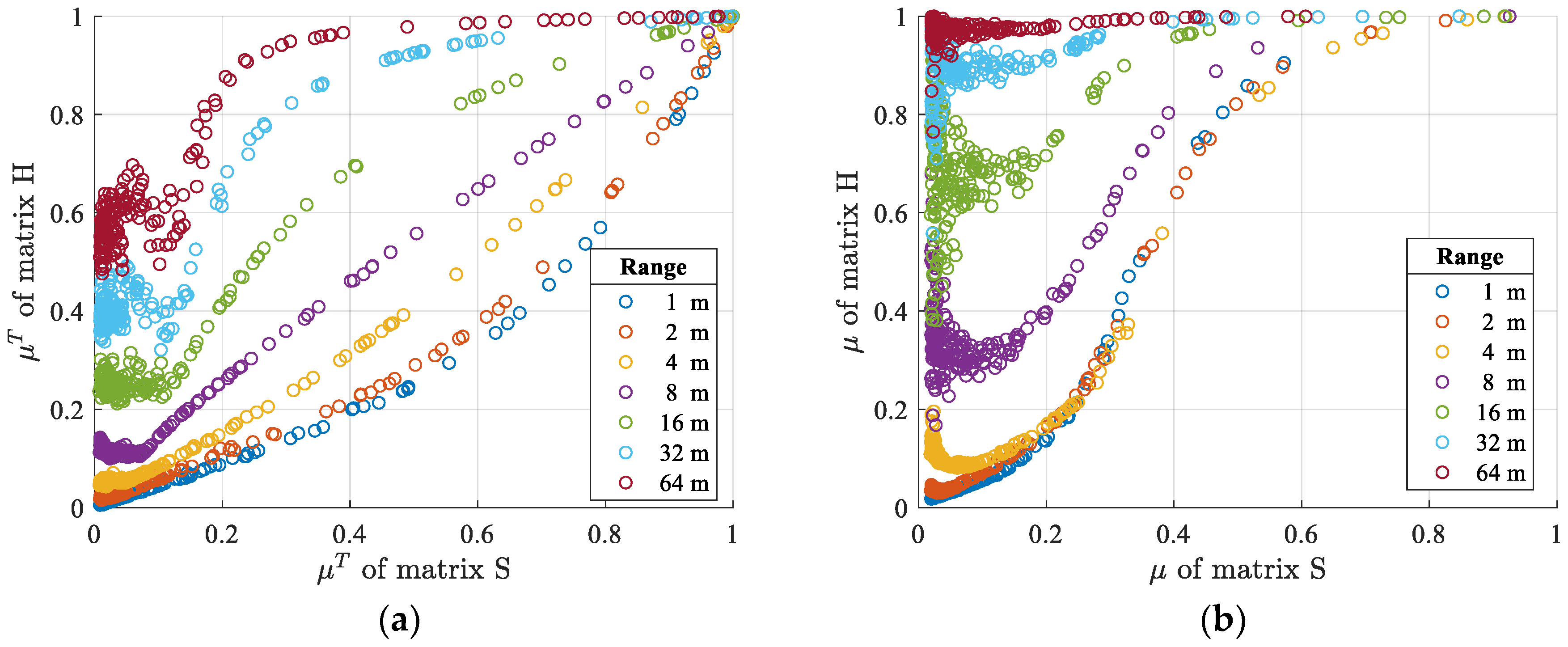
In previous simulations, only one pair of the matrix $\mathbf{H}$ and $\mathbf{S}$ (namely one sample) is generated for validation. In the next, we need to obtain massive samples in which the spectrum of the source goes through the entire low-pass area in the k-space in order to prove that the proposed coherence relationship is still valid in general situation. Therefore, we perform the third numerical simulation in which a set of samples is obtained. In this simulation, the mutual coherences in $\mathbf{H}$ and $\mathbf{S}$ are evaluated by observing the average mutual coherence ${\mu }^{\mathrm{T}}$ that is calculated in rows of the matrix (see Equation (15)). For comparison, the average mutual coherence $\mu$ that is calculated in columns [25]:

$$\mu \left(\mathbf{H}\right)=\frac{{\sum }_{i\ne j}{|{[{\widehat{\mathbf{H}}}^{*}\widehat{\mathbf{H}}]}_{ij}|}^2}{N\left(N-1\right)}$$

(25)

is also observed. ${\mu }^{\mathrm{T}}$ and $\mu$ represent the average level of the coherences in a matrix and thus allow evaluating the coherences more comprehensively. In this simulation, the source is modulated by the random spatial frequencies that are varying in the k-space. In order to obtain sufficient samples, 200 groups of modulation frequencies are generated via Monte Carlo method, while in each group the modulation frequencies are randomly distributed in a low-pass area of which the cut-off spatial frequency is also randomly selected between 0 and the one of the low-pass area at the imaging range of 1 m. If the proposed coherence relationship in matrix form (i.e., Equation (23)) holds for these samples, the average mutual coherences of matrix H and matrix S would be in positive relationship. The results are shown in Figure 4, where (a) demonstrates the relationship ${\mu }^{\mathrm{T}}\left(\mathbf{H}\right)\leftarrow {\mu }^{\mathrm{T}}\left(\mathbf{S}\right)$ and (b) $\mu \left(\mathbf{H}\right)\leftarrow \mu \left(\mathbf{S}\right)$:

Figure 4 shows that the ${\mu }^{\mathrm{T}}$ of matrix H increases with the increasing of the ${\mu }^{\mathrm{T}}$ of matrix S, validating the predicted positive relationship. It is also obvious that in the positive relationship the mutual coherences in the measurement matrix upsurges with the increasing of the imaging range, which can be interpreted by the shrinking spectral low-pass filter. The $\mu$ relationship possesses the same characteristics with ${\mu }^{\mathrm{T}}$, although it represents the coherence level in the column space of the matrix. Therefore, this simulation proves that the proposed coherence relationship is still valid in a general situation.

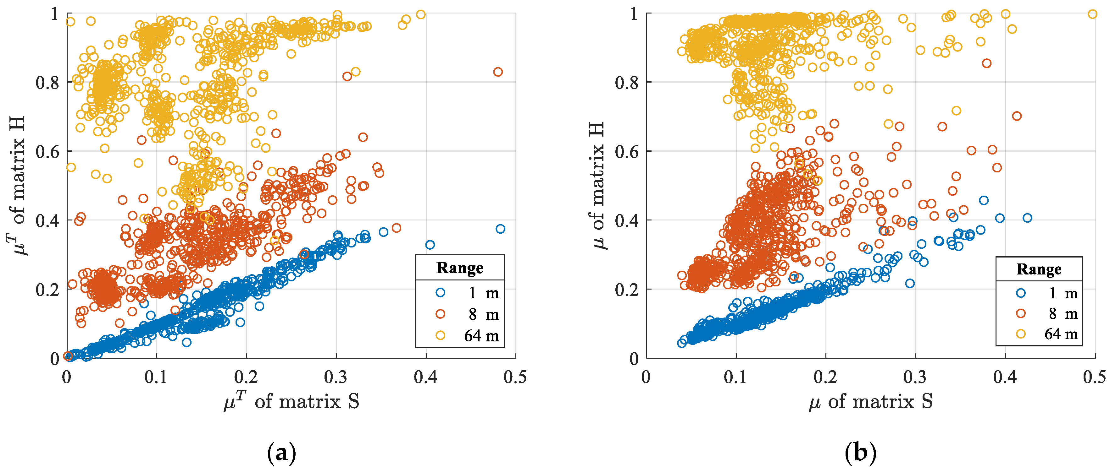
At last, we perform a full-wave simulation in a commercial electromagnetic simulation environment (Ansoft HFSS), in which a set of Complementary Electric-Field-Coupled (CELC) arrays as shown in Figure 5 is introduced in sequence as the radiation source. This simulation shares the same intention with the numerical simulations, although the fictitious sources are replaced with the equivalent sources generated by the near-field scanning of these arrays.

The number of the elements in this set of arrays varies as 25, 100, 225 and 400, while resonant frequencies of the elements are randomly distributed from 26 to 34 GHz. The elements are placed in the same polarization direction. In addition, we randomly select the rows of the source matrix $\mathbf{S}$ and correspoding $\mathbf{H}$ to reassemble a new sample. Eventually, the number of the samples is enlarged to 648. The results are shown in Figure 6, where (a) demonstrates the relationship ${\mu }^{\mathrm{T}}\left(\mathbf{H}\right)\leftarrow {\mu }^{\mathrm{T}}\left(\mathbf{S}\right)$ and (b) $\mu \left(\mathbf{H}\right)\leftarrow \mu \left(\mathbf{S}\right)$:

As is shown Figure 6, the average mutual coherence of $\mathbf{H}$ keeps an approximately linear relationship with the average mutual coherence of S at the imaging range of 1 m. The former coherence obviously upsurges with the increasing of the imaging range. The characteristics of the ${\mu }^{\mathrm{T}}$ and the $\mu$ relationship in this result coincide with previous numerical simulation, validating that the proposed coherence relationship still holds for actual antennas.

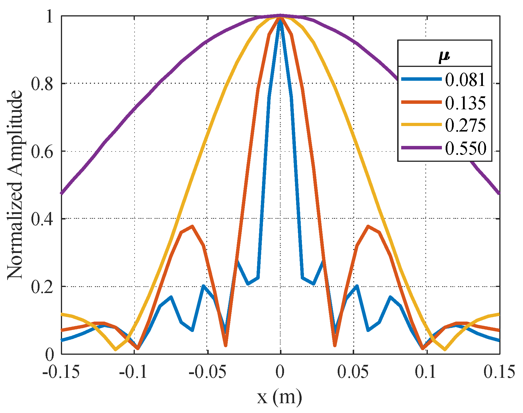
Before we end up with the section of simulation, in order to clearly demonstrate how the coherences in the measurement matrix affect the reconstruction, we generate the point-spread-functions (PSF) of four measurement matrices with the $\mu$ of 0.081, 0.135, 0.275 and 0.550 respectively. These matrices are selected from the samples in previous numerical simulations. The result is shown in Figure 7, where the resolution is significantly improved with the reduction of $\mu$, validating that the number of independent measurements is enlarged by the reduction. Therefore, the reduction of the coherences improves the resolution of microwave computational imaging systems.

The above simulations validate that antennas can be optimized for MCI by reducing the spectral coherences of their equivalent radiation sources; however, it should be noted that how the reduction can be realized on actual antenna structures still remains unknown.

In this paper, we focus on the investigation of the coherence relationship based on antennas’ equivalent radiation sources rather than actual structures. This work is a first step towards the antenna optimization for MCI. The spatial modulation implemented in the numerical simulations avoids overlapping in the k-space by shifting the spectrum, which reduces the spectral coherences. However, at present, this modulation is difficult to implement in practice and will increase requirements in hardwares, which violates the original intention of MCI. For this reason, currently, we do not think the spatial modulation is a practical approach.

Furthermore, if we extend our scope to consider actual antenna structures rather than the equivalent radiation sources, the non-ideal properties, such as mutual couplings between elements, will be great challenges for the formulation. The proposed relationship interprets the generation of the coherences only at the theoretical level because the antennas are replaced with equivalent radiation sources, leaving a research gap between the equivalent sources and actual antennas.

For these reasons, we believe that the investigation of the coherence relationship at an antenna structure level, which permits practical reduction of the coherences, will be a promising and challenging work.

4. Conclusions and Future Direction

The mutual coherences in the measurement matrix are dependent on the mutual coherences of the spatial spectrum of the antennas’ equivalent radiation sources. In this relationship, the imaging scenario functions equivalently as a low-pass filter in the k-space, which limits the spatial frequency of the measurement modes. Growing imaging range narrows this spectral constraint and thus leads to surges in the mutual coherences in the measurement matrix. The minimization of the spatial spectral coherences gives a possible direction for the antenna optimization in MCI applications.

It should be noted that the stationary phase approximation applied in our derivation constraints the spectrum of the modes because it only retains components that contains most of the energy but with low spatial frequency. Applying a more accurate approximation which reserves the terms with high-order phase in Equation (2) maybe an interesting option to extend the spectrum. This is a possible future direction for achieving super-resolution under the inevitable low-pass constraint.