Rolling Bearings Fault Diagnosis Based on Tree Heuristic Feature Selection and the Dependent Feature Vector Combined with Rough Sets

Abstract

Rolling element bearings (REB) are widely used in all walks of life, and they play an important role in the health operation of all kinds of rotating machinery. Therefore, the fault diagnosis of REB has attracted substantial attention. Fault diagnosis methods based on time-frequency signal analysis and intelligent classification are widely used for REB because of their effectiveness. However, there still exist two shortcomings in these fault diagnosis methods: (1) A large amount of redundant information is difficult to identify and delete. (2) Aliasing patterns decrease the methods’ classification accuracy. To overcome these problems, this paper puts forward an improved fault diagnosis method based on tree heuristic feature selection (THFS) and the dependent feature vector combined with rough sets (RS-DFV). In the RS-DFV method, the feature set was optimized through the dependent feature vector (DFV). Furthermore, the DFV revealed the essential difference among different REB faults and improved the accuracy of fault description. Moreover, the rough set was utilized to reasonably describe the aliasing patterns and overcome the problem of abnormal termination in DFV extraction. In addition, a tree heuristic feature selection method (THFS) was devised to delete the redundant information and construct the structure of RS-DFV. Finally, a simulation, four other feature vectors, three other feature selection methods and four other fault diagnosis methods were utilized for the REB fault diagnosis to demonstrate the effectiveness of the RS-DFV method. RS-DFV obtained an effective subset of five features from 100 features, and acquired a very good diagnostic accuracy (100%, 100%, 99.51%, 100%, 99.47%, 100%), which is much higher than all comparative tests. The results indicate that the RS-DFV method could select an appropriate feature set, deeply dig the effectiveness of the features and more exactly describe the aliasing patterns. Consequently, this method performs better in REB fault diagnosis than the original intelligent methods.

1. Introduction

Rolling bearings are the key components of various rotating machinery that are widely used in all walks of life [1,2]. The failure of the bearings could lead to serious consequences such as grave safety accidents, long breaks of production and great pecuniary losses. Thus, accurate status monitoring and timely fault identification of REB is significant for the safe and regular operation of large machinery [3,4]. Accordingly, research and development in REB fault diagnosis has had an all-important social significance and economic value [5,6,7].

In recent years, the researches on rolling bearing fault diagnosis mainly focused on two kinds of methods [7]: (1) Fault diagnosis based on feature extraction and fault recognition; (2) Self-learning and self-evolution fault diagnosis based on deep learning. The first kind of methods firstly obtained fault symptoms from fault signals by signal analysis methods, and then identified fault types through fault recognition methods. Feature extraction [8,9,10] and fault recognition are two determinant steps which affected the accuracy of fault diagnosis. Therefore, the related researches mainly focused on feature extraction method [11,12] and fault recognition method. The second kind of methods [13] did not need advance feature extraction and could learn complex fault parameters from the original fault data and realize fault identification autonomously. The related researches mainly focused on deep neural network and various deep learning methods based on it.

Signal processing is the most effective and widely used method for fault feature extraction and is the significant basis for machinery fault diagnosis. Recently, many kinds of signal analysis methods have been widely used in fault diagnosis, such as wavelet [14,15], empirical mode decomposition (EMD) [16,17], variational mode decomposition (VMD) [18,19] and singular value decomposition (SVD) [20,21]. They are the most important signal analysis methods in REB fault diagnosis because of their prominent effectiveness. After a long time of in-depth research by a large number of scientists, these signal analysis methods all could obtain good enough fault feature of rolling bearings. In addition, intelligent algorithms are another key technology for fault diagnosis, and a variety of such algorithms [9,22,23,24], such as support vector machine [9,22], clustering algorithms [23], neural networks [24] and so on, are used to design and improve the intelligent fault diagnosis system. Signal processing and an intelligent classification algorithm cooperate efficiently in REB fault diagnosis.

With the capacity of automatically learning complex features of input data, deep learning architectures have great potential to overcome drawbacks of traditional intelligent fault diagnosis. Accordingly, deep learning algorithms have been applied widely in machine health monitoring recently [2]. Duy-Tang Hoang [2] proposed a method for diagnosing bearing faults based on a deep structure of convolutional neural network, and this method has high accuracy and robustness in noisy environment. With deep convolutional neural network as the main structure, Xiang Li [13] proposed a novel domain adaptation method for rolling bearing fault diagnosis. It minimized the maximum mean deviation between the source domain and the target domain in multi-core structure, and significantly improved the performance of cross-domain testing. An integrated deep learning diagnosis method based on multi-objective optimization is proposed by Sai Ma [5]. This method weighted and integrated convolutional residual network (CRN), belief network (DBN) and depth automatic encoder (DAE) to realize effective diagnosis of bearing faults. Zhiyu Zhu [6] presented a capsule network with an inception block and a regression branch, which improved the generalization ability of deep neural network. Wentao Mao [25] designed a deep output kernel learning method to conduct collaborative diagnosis of multiple bearing fault types, which improved the generalization ability and robustness of the diagnosis model. Shao Haidong [26] proposed an integrated depth automatic coding method to overcome the dependence of traditional artificial feature extraction methods on depth learning models and the limitations of some depth learning models.

However, there still exist two shortcomings in traditional REB fault diagnosis methods: (1) A large amount of redundant information is difficult to identify and delete [27]. (2) Aliasing patterns decrease the classification accuracy [27] and increase the complexity of fault diagnosis. Although deep learning techniques could extract more representative features from bearing fault data adaptively, they usually have high computational cost, slow convergence speed and unavoidable randomness [25].

To overcome these two shortcomings in traditional REB fault diagnosis methods, this paper proposes an improved intelligent fault diagnosis method for REB. The major contributions of this work are as follows: (1) An adaptive fault description model is established based on RS-DFV, (2) a rough set is used to enhance the description accuracy and the self-healing nature of RS-DFV, and (3) a tree heuristic feature selection method is devised to delete the redundant information and construct the structure of RS-DFV. Therefore, the fault diagnosis method presented in this paper ameliorated the algorithm performance in terms of accuracy, complexity as well as timeliness and greatly advanced the efficiency and practicability of REB fault diagnosis.

To improve the validity and timeliness of REB fault diagnosis, the researchers designed a fault diagnosis method based on RS-DFV for REB. The current study’s discourse is composed as follows: Section 2 recounts the conception of RS-DFV, the tree heuristic feature selection method (THFS) and the RS-DFV extraction method. The evaluation of the feature vector and the classifier are introduced in Section 3. In Section 4, the REB fault diagnosis tests are described in detail, and the experimental results are analyzed and discussed. At last, the conclusions of this study are arranged in Section 5.

2. Materials and Methods

2.1. The Framework of REB Fault Diagnosis Based on THFS and RS-DFV

The fault diagnosis method based on THFS and RS-DFV proposed in this paper includes two crucial components: (1) a unique feature selection method (THFS) which is not only need to remove the redundant features to the maximum extent, but also must determine the composition of DFV and established the logical structure of DFV; (2) a feature organization method (RS-DFV) which could not only overcome the interference of overlapping samples, dig out the complex relationship between faults and features, but also improve the accuracy of fault representation. The framework of REB Fault diagnosis based on THFS and RS-DFV is showed in Figure 1.

2.2. The Proposition of RS-DFV

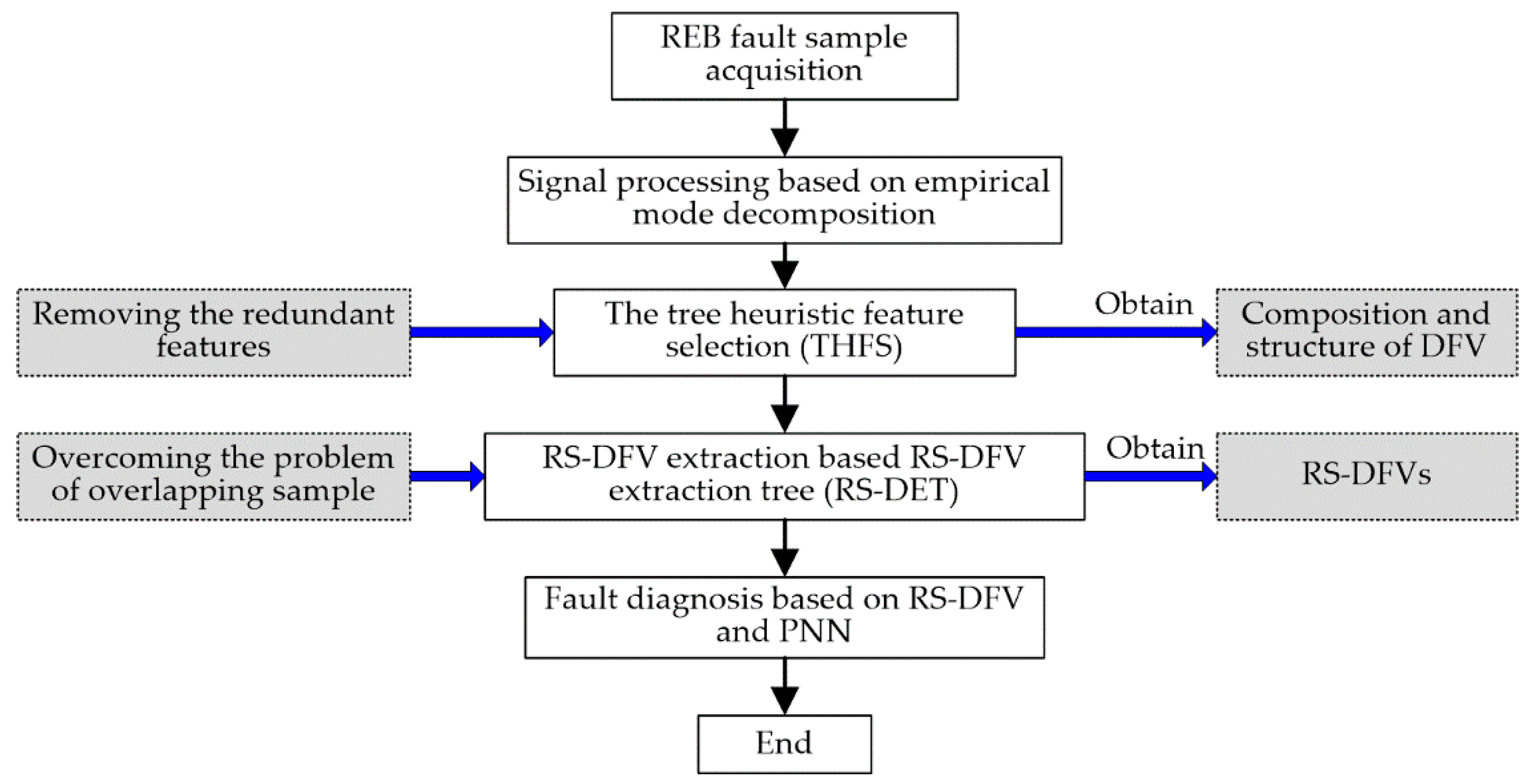
2.2.1. The Basic Concept of DFV

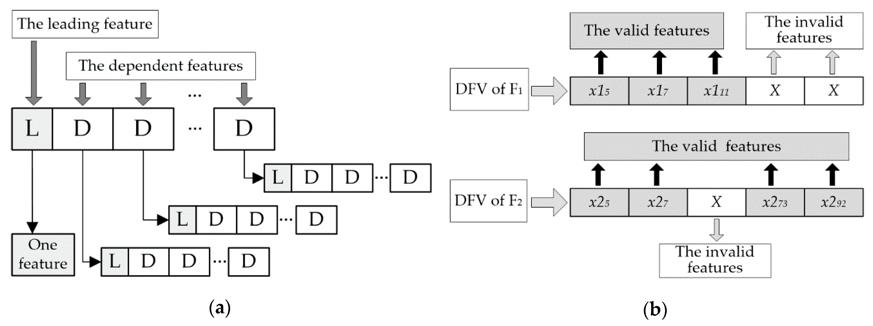
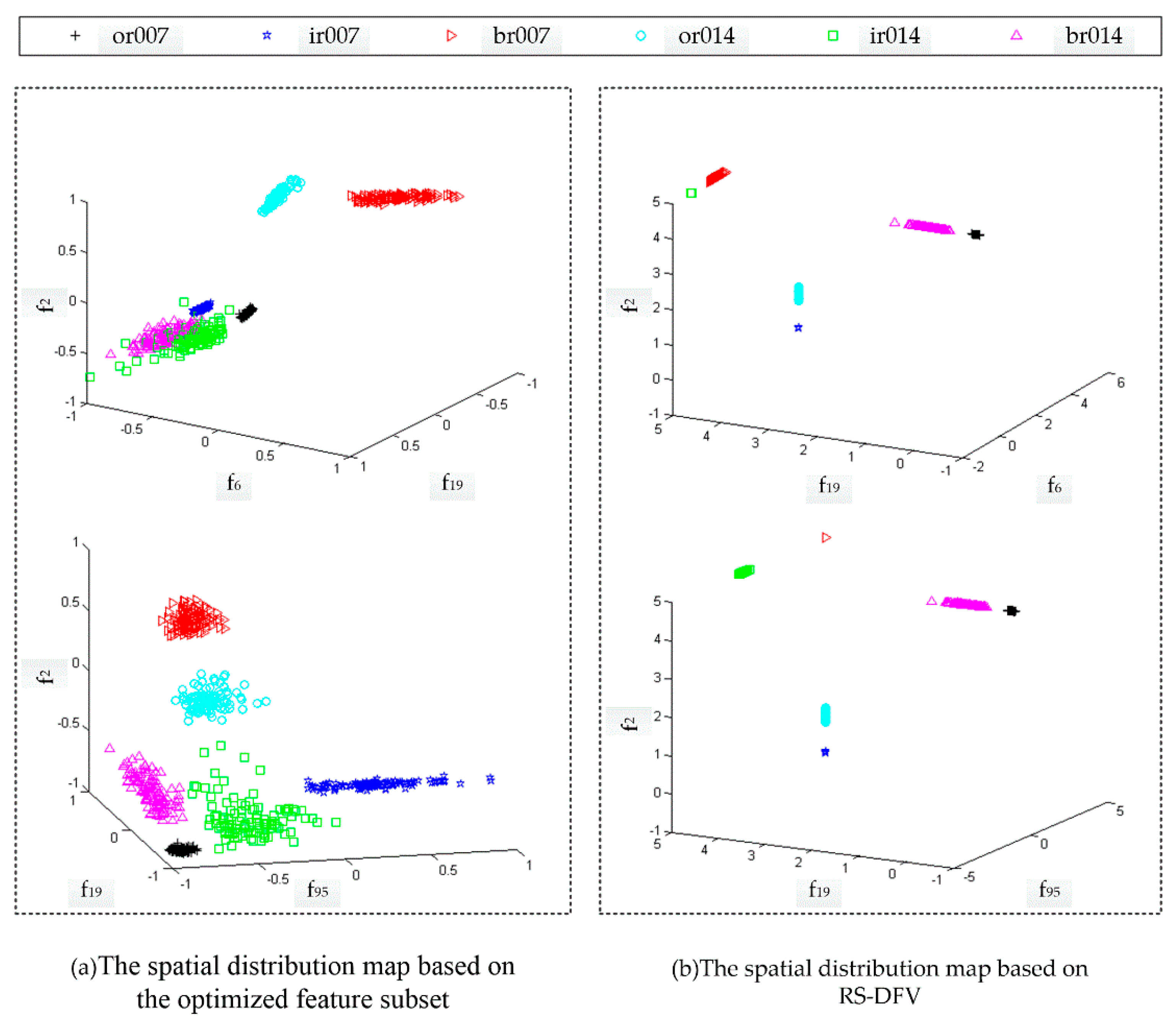
To simulate the object description method of the human brain, one study [22] designed a special feature vector that was called dependent feature vector (DFV) for REB fault description. The topology and logical structure of DFV is displayed in Figure 2a. In DFV, there must be at most one leading feature (LF). However, A DFV could include many dependent features (DFs) or no DF. DFV could mining the essential difference among all kinds of faults through its unique nested structure. Moreover, the difference between different faults is magnified by the means of adaptive invalid features of the DFV, and the difference among faults of the same type is reduced at the same time, as illustrated in Figure 2b and Equations (1)–(7). Therefore, DFV greatly improved the accuracy of fault description and fault diagnosis.

In a DFV, the valid features must be acquired through the analysis of sample data. However, invalid features do not have to be calculated, and it is only necessary to subjectively give an effective value for them. The unified evaluation mechanism of invalid items in a DFV could greatly improve its fault discrimination.

For the examples in Figure 2b, F1 and F2 are two different fault types, xi_j is the jth feature item of the fault Fi, $\left|{fv}_1-f{v}_2\right|$ is the Euler distance between F1 and F2 based on the traditional feature vector, and $\left|DF{V}_1-DF{V}_2\right|$ is the Euler distance between F1 and F2 based on the DFV. As long as the value (X) of the invalid features is suitable, Equations (3) and (4) are true. It is obvious that the DFV could magnify the difference between different faults through the value assignment of the invalid features.

$${\left|{fv}_1-f{v}_2\right|}^2={(x{1}_5-x{2}_5)}^2+{(x{1}_7-x{2}_7)}^2+{(x{1}_{11}-x{2}_{11})}^2+{(x{1}_{73}-x{2}_{73})}^2+{(x{1}_{92}-x{2}_{92})}^2$$

(1)

$${\left|DF{V}_1-DF{V}_2\right|}^2={(x{1}_5-x{2}_5)}^2+{(x{1}_7-x{2}_7)}^2+{(x{1}_{11}-X)}^2+{(X-x{2}_{73})}^2+{(X-x{2}_{92})}^2$$

(2)

$$\{\begin{array}{l}{(x{1}_{11}-X)}^2\gg {(x{1}_{11}-x{2}_{11})}^2\\ {(X-x{2}_{73})}^2\gg {(x{1}_{73}-x{2}_{73})}^2\\ {(X-x{2}_{92})}^2\gg {(x{1}_{92}-x{2}_{92})}^2\end{array}$$

(3)

$$\left|DF{V}_1-DF{V}_2\right|\gg \left|f{v}_1-f{v}_2\right|$$

(4)

$${\left|f{v}_{11}-f{v}_{12}\right|}^2={(x11_5-x12_5)}^2+{(x11_7-x12_7)}^2+{(x11_{11}-x12_{11})}^2+{(x11_{73}-x12_{73})}^2+{(x11_{92}-x12_{92})}^2$$

(5)

$${\left|DF{V}_{11}-DF{V}_{12}\right|}^2={(x{11}_5-x{12}_5)}^2+{(x{11}_7-x{12}_7)}^2+{(x{11}_{11}-x{12}_{11})}^2+{(X-X)}^2+{(X-X)}^2$$

(6)

$\left|f{v}_{11}-f{v}_{12}\right|$ is the Euler distance between two faults of type F1 based on the traditional feature vector, and $\left|DF{V}_{11}-DF{V}_{12}\right|$ is the Euler distance between two faults of type F1 based on DFV. No matter what is the value (X) of the invalid features, Equation (7) is true. Obviously, the DFV was able to significantly lessen the discrepancies among the same faults.

$$\left|DF{V}_{11}-DF{V}_{12}\right|<\left|f{v}_{11}-f{v}_{12}\right|$$

(7)

2.2.2. The Tree Heuristic Feature Selection

• Feature evaluation based on information granulation and neighboring clustering

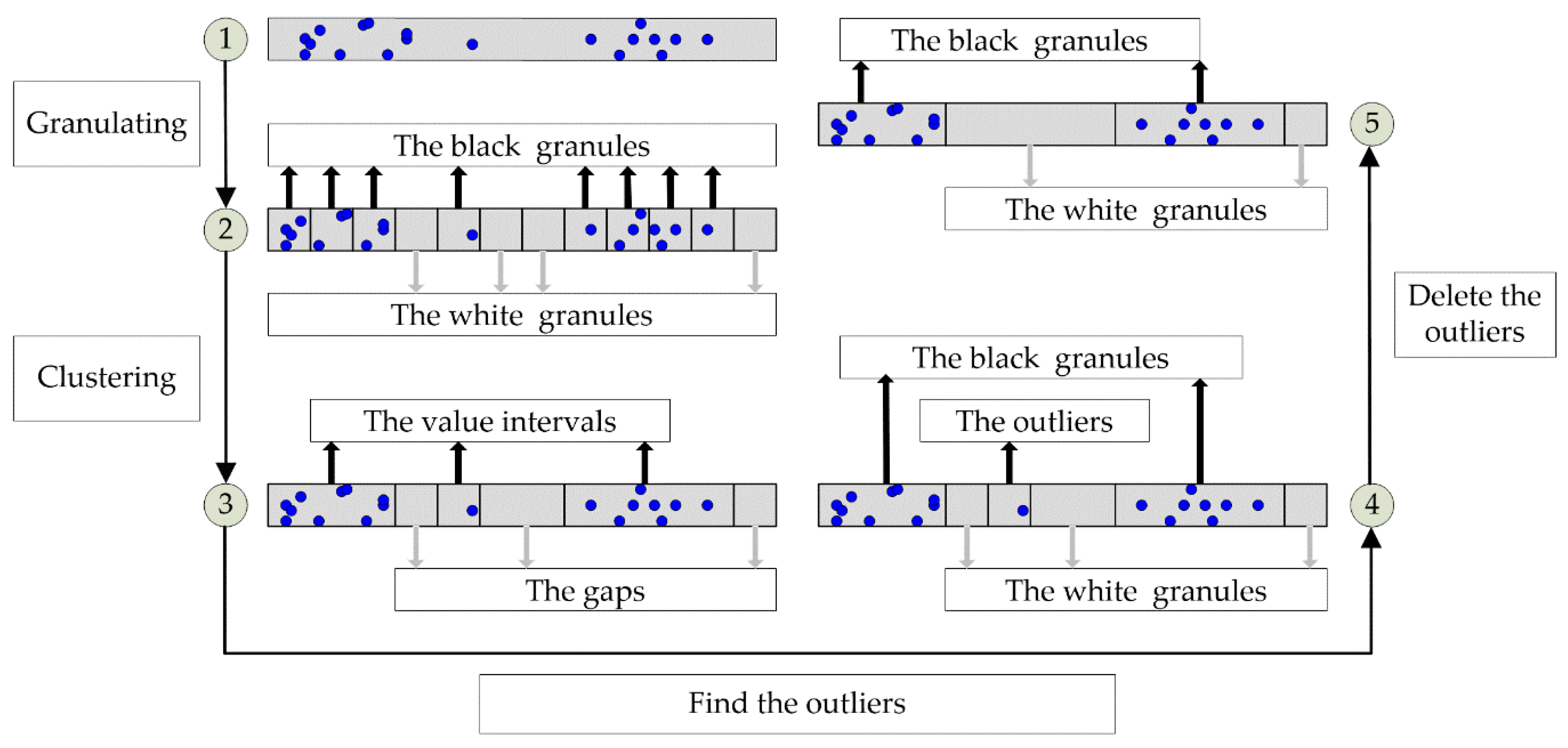
Different feature selection methods required different feature evaluation criteria, but the excellent traditional feature evaluation methods could not provide the best heuristic knowledge for the feature selection method proposed in this paper. So, a feature evaluation method based on information granulation and neighboring clustering is put forward for tree heuristic feature selection (THFS). In this feature evaluation method, information granulation and neighboring clustering were used to delete the features that were obviously ineffective in fault distinguishing at first; then, the remaining features were evaluated through Equations (8)–(11). The specific steps of this feature evaluation method are introduced below.

Step 1: The value range of one feature is divided into many small granules evenly in accordance with the same criterion, as illustrated in Figure 3①–②. The granules that included some feature values of samples are black granules, and the others are white granules.

Step 2: The adjoining granules of the same type are merged to a larger one through the neighboring clustering method, as illustrated in Figure 3②–③. The black granules that included very few samples and the white granules with a tiny length are outliers (Figure 3④).

Step 3: The black outlier is first changed to be white and amalgamated with white granules adjacent to it. Then, the white outlier is changed to be black and amalgamated with black granules adjacent to it, as illustrated in Figure 3④–⑤.

Step 4: If there is only one black granule or two different black granules both with some samples of the same type, this feature is considered to be ineffective in fault distinguishing and deleted.

Step 5: The remaining features are evaluated through Equations (8)–(11):

$$L_i{=x}_i{}^{+}-x_i{}^{-}$$

(8)

$$L_{i(i+1)}{=x}_{i+1}{}^{-}-x_i{}^{+}$$

(9)

$$V_{i(i+1)}=\frac{L_{i(i+1)}}{\frac{1}{2}(L_i+L_{i+1})}$$

(10)

$$P(x)={\displaystyle \sum _i^{N-1}{V}_{i(i+1)}}$$

(11)

where L_i is the length of the No. i black granule, x_i⁺ is its upper bound, and x_i⁻ is its lower bound. L_i (i+1) is the length of the white granule between the No. i and No. (i+1) black granules. V_i (i+1) is the separability between the No. i and No. (i+1) black granules, and N is the number of the black granules. P(x) is the score of this feature, and a large P(x) displayed its high separability among the black granules.

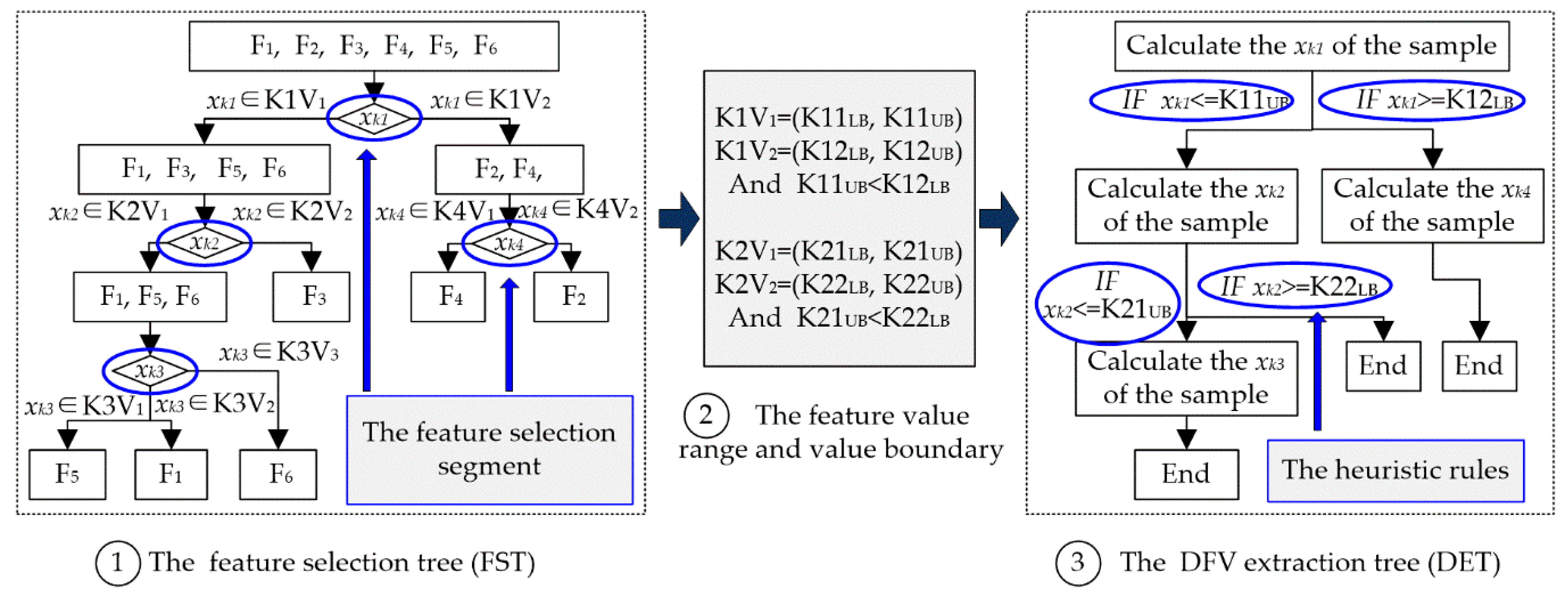
• Feature selection based on the tree heuristic search strategy

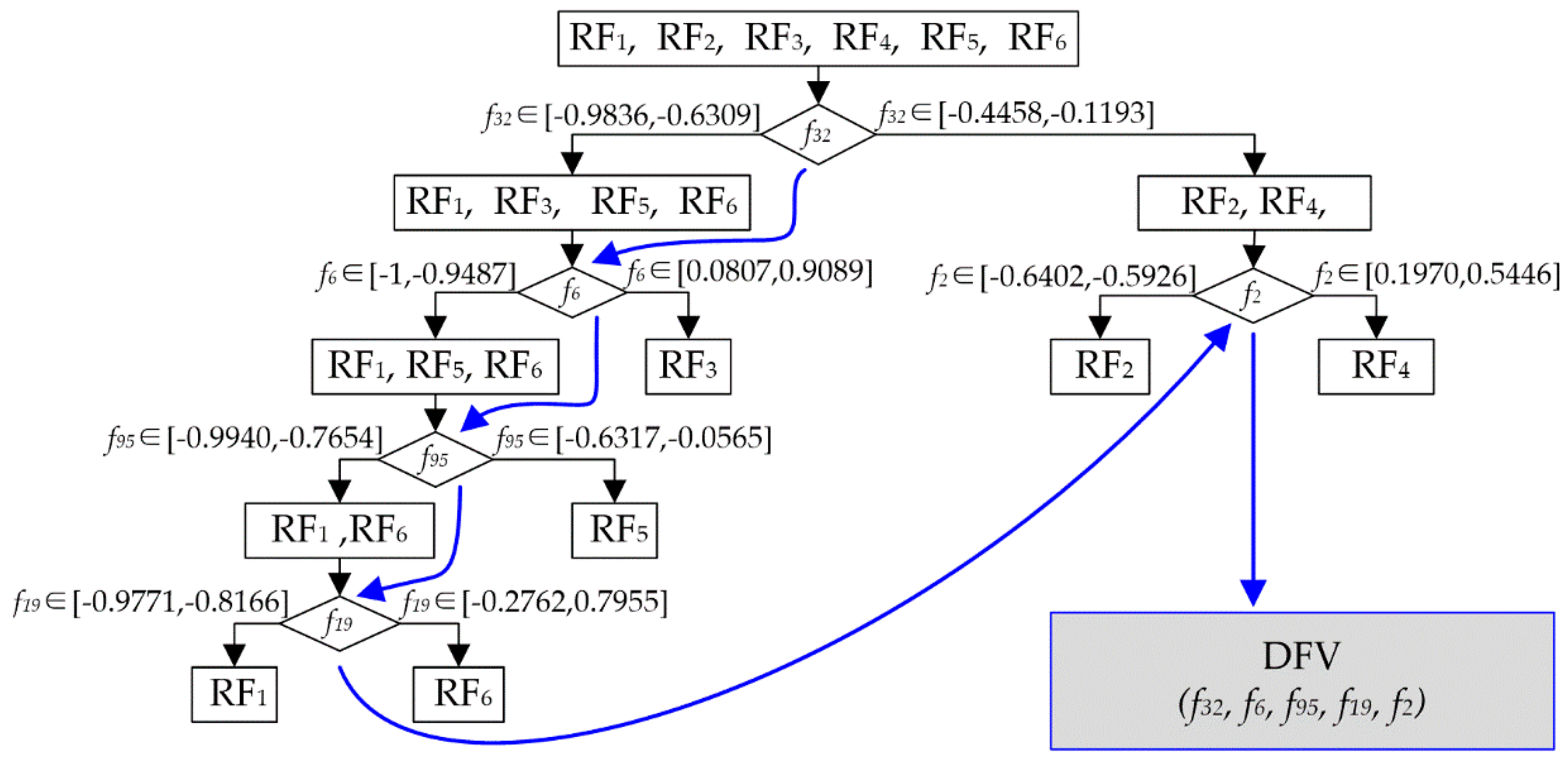
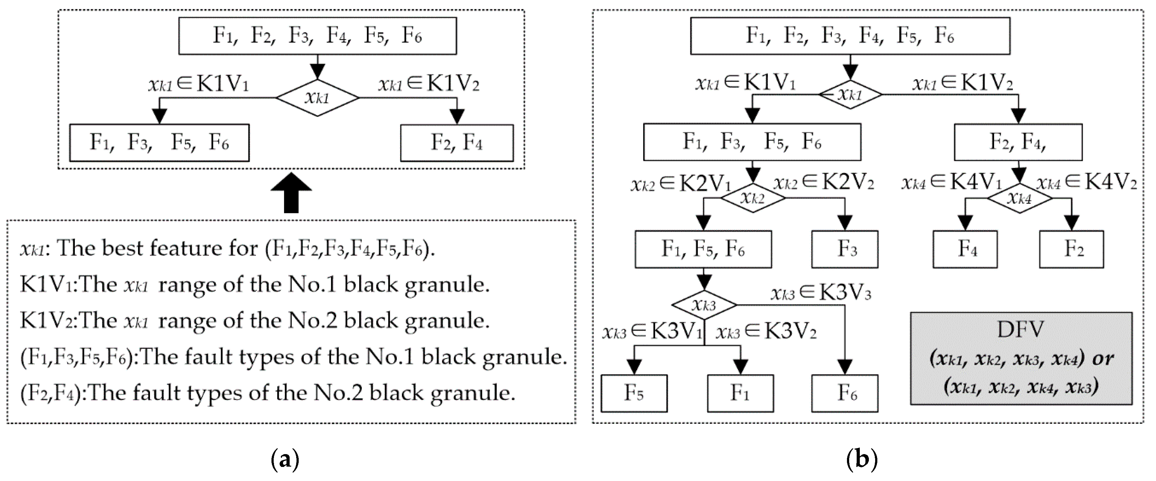
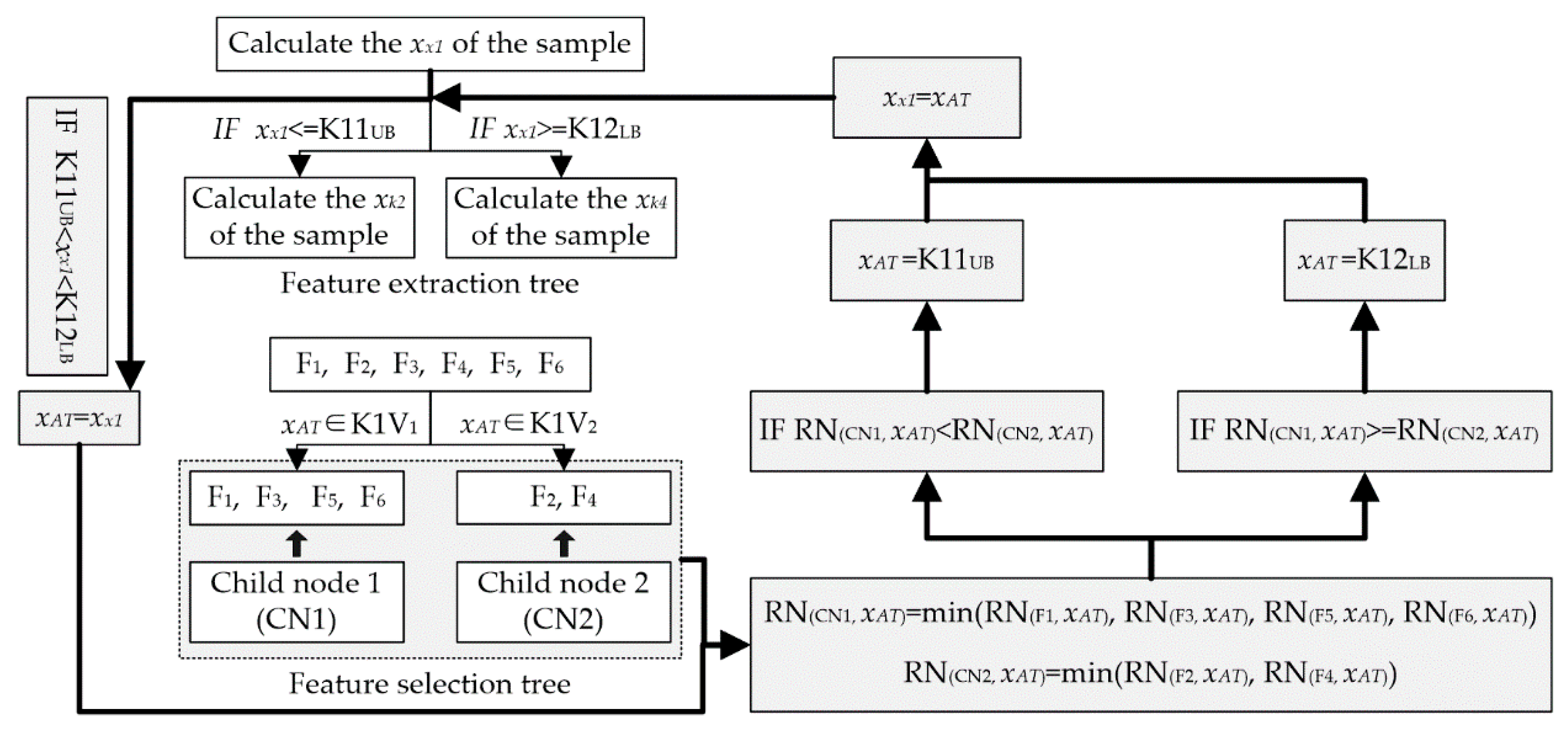
The structure establishment of the feature vector is a very important basis for DFV. To adapt to the uniqueness of DFV, this study proposes a feature selection method based on THFS to establish the structure of DFV. The workflow of THFS is illustrated in Figure 4.

The most efficient feature (x_k1) for the sample space is first chosen through the feature evaluation method based on information granulation and neighboring clustering, which is introduced above, and the black granules are obtained. Each black granule includes some fault types, and the samples of these types make a fault subspace. Then, the sample space is made the root node, the subspaces are made the leaf nodes, and the x_k1 value range of each leaf node is marked. Thus, the local structure connected to the root of the heuristic tree is established, as illustrated in Figure 4a. If a leaf node includes faults of more than one type, its subtree is built using the same method. When all leaf nodes contain faults of only one type, the heuristic tree has completed its growth and gained complete tree, as illustrated in Figure 4b.

The optimization feature subset is obtained through traversing the heuristic tree. Because the position of each feature in a DFV is fixed, traversing the heuristic tree with a different method could get a different DFV. For example, in Figure 4b, depth-first traversal of the heuristic tree could get a DFV (x_k1, x_k2, x_k3, x_k4), but breadth-first traversal could get another DFV (x_k1, x_k2, x_k4, x_k3). Therefore, THFS not only has completed the feature selection and the optimization of feature subset but also could establish the structure of the DFV.

2.2.3. RS-DFV Extraction

• DFV Extraction Tree

Extracting the DFV of fault samples is another key step of the fault diagnosis method presented in this paper. The DFV is different from the traditional feature vector because of its unique structure. In a DFV, the importance of each feature item is not equal: some of them are valid feature items, and the others are invalid. More importantly, faults of different types had different valid feature items and invalid feature items, i.e., the same feature is of different importance for different faults. In addition, only the valid feature items of DFV need to be calculated from the sample data and the value of the invalid items are set subjectively, based on the requirement of the fault classification. All these differences considerably increased the difficulties of DFV extraction. Moreover, for a fault sample that has to be diagnosed, features that are valid items in the sample’s DFV are unknown. This made the DFV extraction more difficult.

To overcome those problems in the DFV extraction mentioned above, a tree heuristic feature extraction method is put forward to extract the DFV in this paper, as illustrated in Figure 5.

First, a DFV extraction tree (DET) that inherited the heuristic rules of the feature selection tree (FST) is put forward in this paper, as illustrated in Figure 5③. The DET is constructed based on the FST: (1) The FST is traversed. When a non-leaf node is passed, continue; when a feature selection segment is passed, a feature calculation node for the DET is built; when a leaf node is passed, an end-node for the DET is built. (2) A connection relationship is established among the nodes for the DET, and consistency with the FST is ensured. (3) According to the value ranges of the child nodes that had the same parent node in the FST, heuristic rules that could guide the subsequent feature calculation for the DET are built.

Then, for a new fault sample, the values of all valid feature items are calculated in turn according to the guidance of the (DET); hence, the valid feature items of the DFV are obtained. As illustrated in Figure 6, different faults have different valid features, but their valid features all could be accurately calculated through DET.

Finally, the other feature items in the DFV are the invalid feature items of this fault sample, and all invalid features are subjectively assigned the same specific value. Therefore, the DFV of all fault samples could be acquired in this manner.

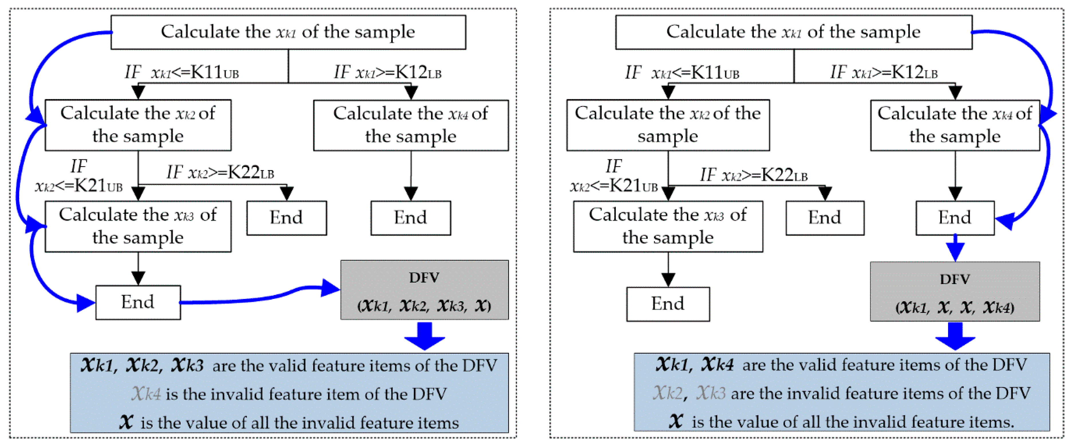
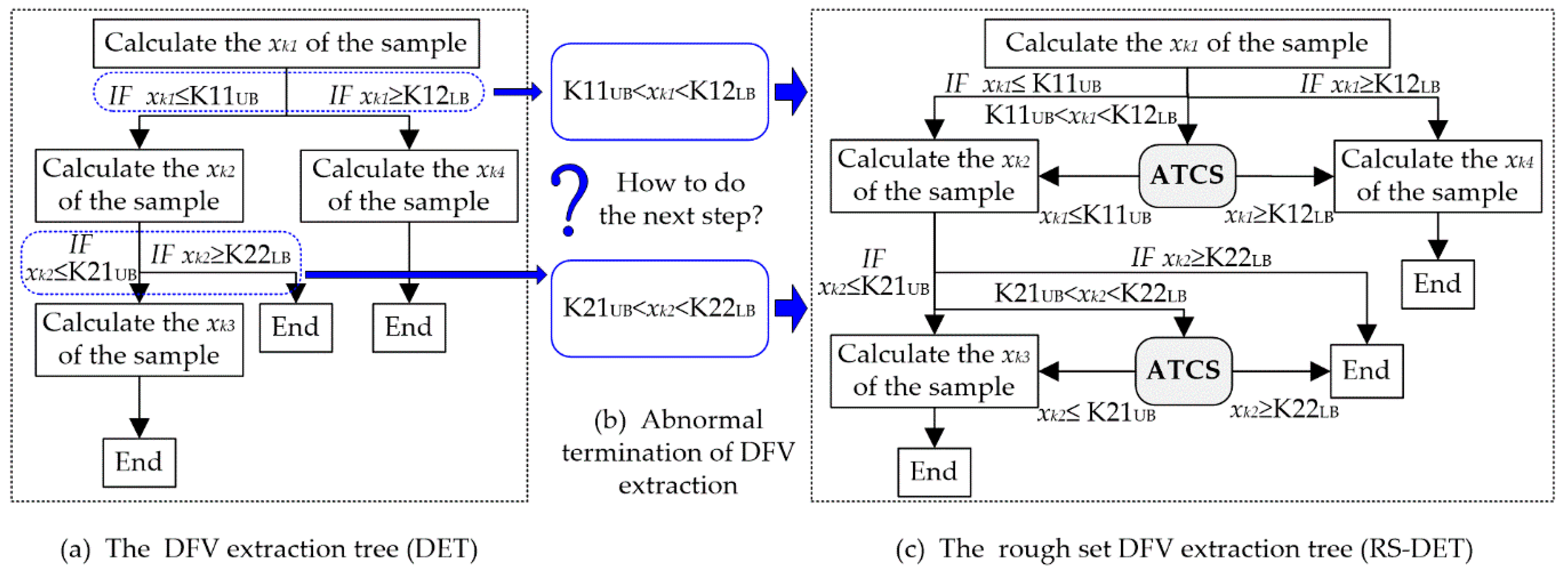
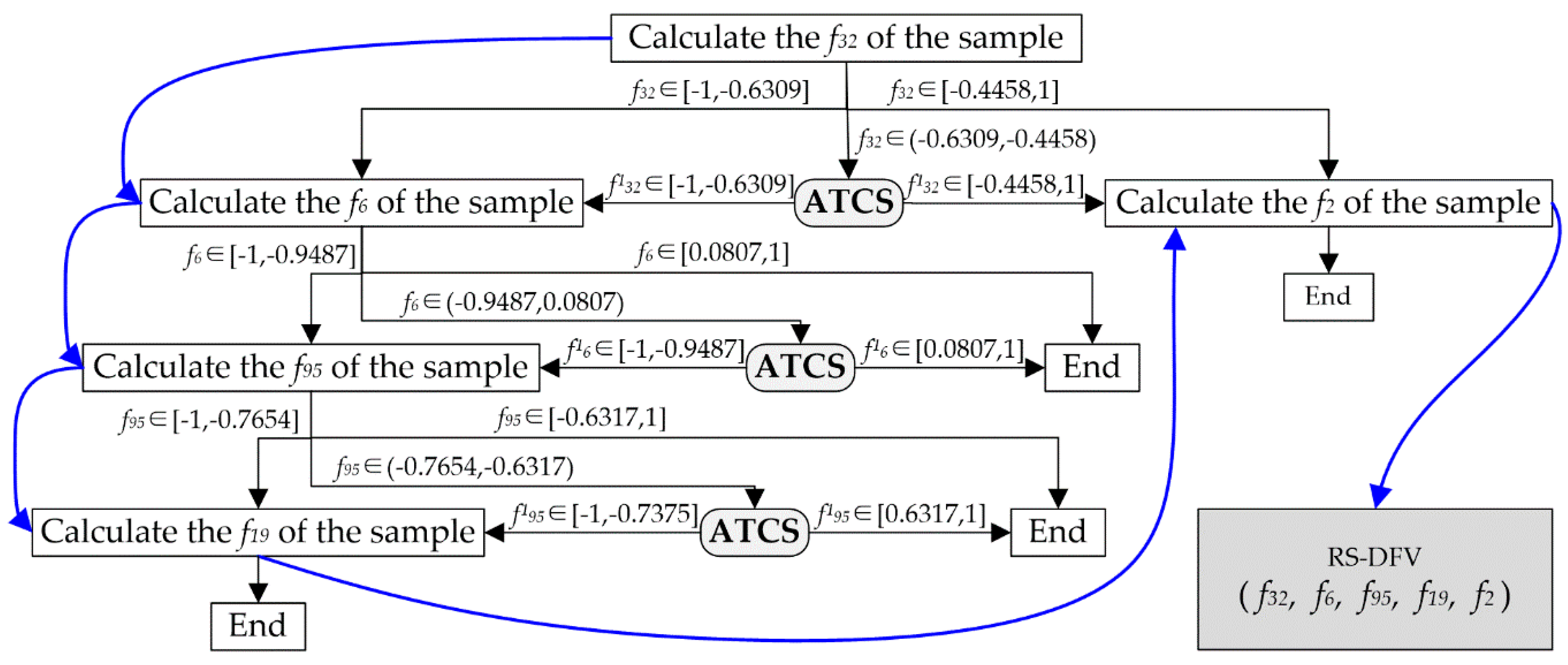
• RS-DFV Extraction Tree

Although the tree heuristic feature extraction method overcomes the difficulties in DFV extraction, it could efficiently and accurately start the calculation of an unknown fault sample and successfully calculated the DFV of most of the fault samples. However, there is still another weakness in the DFV: The feature value obtained in the parent feature calculation node of the DFV extraction tree could not meet the demand of any one heuristic rule connected to this feature, and there is be no inspire information for the next step, as illustrated in Figure 7a,b. This could lead to an abnormal termination in the DFV extraction and inaccurate calculation of the sample DFV.

To overcome the problem mentioned above, a rough set is introduced to solve the boundary problem of heuristic rule in the DFV extraction tree, and a DFV extraction method based on the rough set and the DFV extraction tree is presented in this paper. As illustrated in Figure 7c, a new DFV extraction tree combining the rough set and DET (RS-DET) is designed. The RS-DET increased an abnormal termination correction segment (ATCS) for each node that had more than one child nodes. When an abnormal DFV extraction termination occurred, the corresponding ATCS responded quickly and reasonably amended the value of the current heuristic feature to be instructive. Obviously, RS-DET could effectively overcome the abnormal suspension of DET and was able to complete the DFV extraction of each sample. The procedure of the ATCS is displayed below.

Step 1: Extract the DFV in accordance with the instructions of the RS-DET until an abnormal termination appeared, record the current fault sample as an AT fault sample, record the current node as an ATN, and record the current heuristic feature as an AT feature (x_AT).

Step 2: Find the all child nodes of the ATN in the RS-DET and put them into the node set CN-ATN.

Step 3: For each node in CN-ATN, find fault types that were included in it, construct a rough set on x_AT for each fault type, and calculate the roughness of this node based on Figure 8 and Equations (12)–(14).

Step 4: Amend the value of x_AT according to the roughness of the child nodes illustrated in Figure 9 and Equations (12) and (13).

Step 5: Go back to step 1.

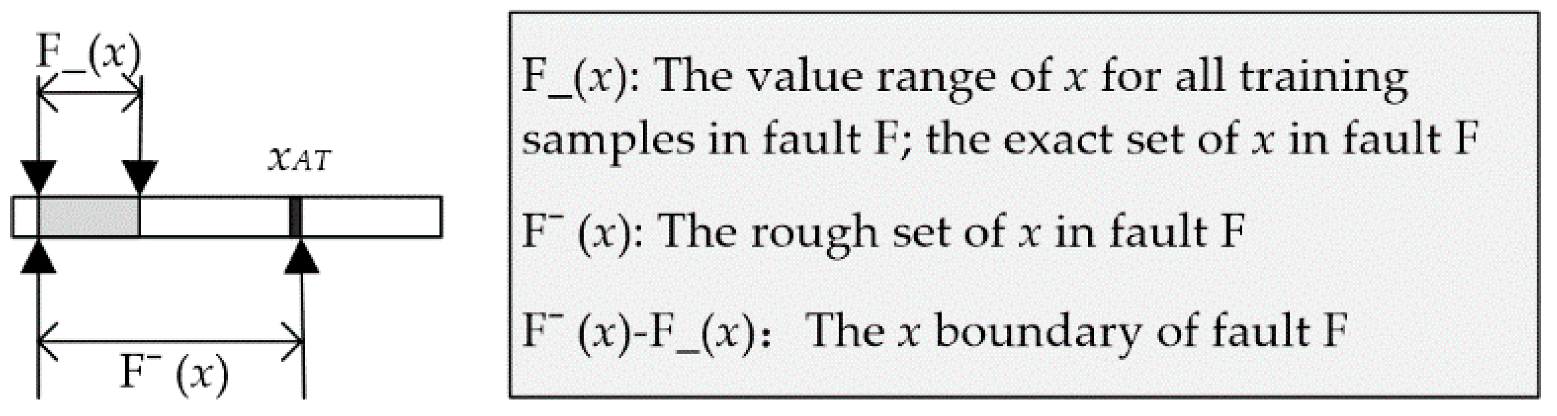
• Feature Correction based on the Rough Set

The ATCS could overcome the problem of abnormal termination in DFV extraction; hence, it is a most important part in RS-DET. In this paper, a rough set is applied to amend the current heuristic feature.

First, the fault sample that caused an abnormal termination is treated as a fault sample in fault type F, and the rough set of F is obtained through the method illustrated in Figure 8. F_-(x) is the value range of the current heuristic feature for all the training samples in fault type F, and RN(F, xAT) is the roughness of fault type F based on the current heuristic feature. Through Equation (12), the roughness of every fault type based on the current heuristic feature could be acquired. Then, for the child nodes of the ATD, RN(CNh, xAT) is the roughness of the hth child node, and, as illustrated in Equation (13), RN(CNh, xAT) is the minimum roughness of all fault types in the hth child node. Finally, the child node that included the fault type with the minimum roughness is found, the value range (X) of the current heuristic feature for all the training samples in this child node is obtained, and the value of xAT toward X is amended based on Equation (14). Therefore, the ATCS solved the problem of abnormal termination in DFV extraction and made it possible for DFV extraction to be accurately completed.

$$RN(F,x_{AT})=\frac{F^{-}(x)-F_{-}(x)}{F_{-}(x)}$$

(12)

$$RN(C{N}_h,x_{AT})=min(RN(F_{h1},x_{AT}),RN(F_{h2},x_{AT}),\cdots ,RN(F_{h3},x_{AT}))$$

(13)

$$x_{AT}=\{\begin{array}{c}min(X),x_{AT}<min(X)\\ max(X),x_{AT}>max(X)\end{array}$$

(14)

2.3. The Evaluation of the Feature Vector and the Classifier

2.3.1. The Evaluation of Feature Vector

Euclidean distance is widely used to evaluate feature sets in fault diagnosis. The average Euclidean distance presented by Equation (15) is put forward in this paper to confirm the superiority of the THFS and RS-DFV. The average Eulerian distance among different fault types reflected the dispersion among different faults, and the average Eulerian distance among the faults of the same type could measure the compactness of this fault.

$$d_{ij}=\frac{1}{h\times k}{\displaystyle \sum _{m=1}^h{\displaystyle \sum _{n=1}^{k}MSE(i(m),j(n))}}$$

(15)

The average Euclidean distance between the ith fault type and the jth fault type is d_ij; the Euclidean distance between fault Fi and fault Fj is MSE(Fi, Fj); i(m) is the mth fault of the ith fault type, and j(n) is the nth fault of the jth fault type. h is the fault number of the ith fault type; and k is the fault number of the jth fault type.

$$D{A}_{i(min)}=\frac{min\left(d_{ij}\right)}{d_{ii}}(j=1,2,\cdots ,cn;j\ne i)$$

(16)

$$D{A}_{i(ave)}=\frac{\frac{1}{cn-1}\left({\displaystyle \sum _{j=1,j\ne i}^{cn}{d}_{ij}}\right)}{d_{ii}}$$

(17)

Then, another parameter, DA, is presented to measure the fault distinguishing ability of feature vectors, as depicted by Equations (16) and (17). DA_i(min) is the worst distinguishing ability of the feature vector for the ith fault. DAi(ave) is the average distinguishing ability of the feature vector for the ith fault; d_ij is the average Euclidean distance between the ith fault type and the jth fault type; d_ii is the average Euclidean distance among all faults of the ith fault type; min(_dij) is the minimum Euclidean distance between the ith fault type and others; cn is the number of fault types. DA_i(min) and DA_i(ave) not only considered the dispersity among different faults but also comprised the compactness of one fault. Therefore, DA_i(min) and DA_i(ave) could well reflect the fault distinguishing ability of feature vectors. The bigger the values of DA_i(min) and DA_i(ave), the better the fault distinguishing ability of the feature vector.

2.3.2. The Intelligent Fault Classification Method

The fault classification method is another significant determinant factor for the timeliness and accuracy of fault diagnosis. Thus, it is crucial in designing a suitable fault classification method according to the specificity of the faults and the feature vector.

For the REB fault diagnosis discussed in this study, the unique feature vector DFV not only had a very simple structure but also made the corresponding relation between the feature vectors and REB faults absolutely clear. In this case, the general classifiers all could get the satisfactory accuracy rate for the fault classification, such as BP, RBF, PNN, SVM and so on. By comparison, PNN is easy to train, has a better real-time performance, has a simpler structure and the calculation of PNN is simpler and faster [23]. Most importantly, the PNN was proved to be very suitable for classification problems of this type [23]. Consequently, this paper chose the PNN to design the intelligent fault classification method.

The probabilistic neural network (PNN) based on the Parzen probabilistic density function and the Bayesian classification rule was proposed by Specht [24]. The PNN had four layers, namely the input layer, the pattern layer, the summation layer and the output layer, and its basic structure is illustrated in Figure 10. As found in many studies [22,23], the PNN is not only easy to train but also very excellent in timeliness. Furthermore, in the case of sufficient training samples, the PNN could get the optimal classification results. This is only a brief introduction of the PNN theory, and the detailed explanation was given by Specht (1990) [24].

3. The Digital Simulation

3.1. The Fault Data of Rolling Element Bearings

In this section, the proposed method (RS-DFV) is applied to REB fault diagnosis. Besides, the experimental fault data of the paper comes from the Bearings Vibration Dataset of Case Western Reserve University [25,26,27]. As showed in Figure 11, the test stand consists of a 2 hp motor (left), a torque transducer/encoder (center), a dynamometer (right), and control electronics (not shown). The test bearings support the motor shaft. Single point faults were introduced to the test bearings using electro-discharge machining. Vibration data was collected using accelerometers, which were attached to the housing with magnetic bases. Accelerometers were placed at the 12 o’clock position at the drive end of the motor housing. The signals of this this dataset are collected at 48,000 samples/s under 2 hp load, the defect sizes are 0.007 or 0.014 in, and this dataset does not contain data without failure. In this paper, each original fault signal is truncated into 118 fault samples that are presented in

Table 1. The data set of the rolling element bearings.

Label of Class	Position of Fault	Defect Size (in.)	The Number of Fault Samples
RF1	Outer race	0.007	118
RF2	Inner race	0.007	118
RF3	Ball	0.007	118
RF4	Outer race	0.014	118
RF5	Inner race	0.014	118
RF6	Ball	0.014	118

.

3.2. The Flow of the Fault Diagnosis Experiment

The application experiments were conducted according to Figure 1.

First, each fault sample was decomposed through EMD, and the 20 feature parameters presented in

Table 2. The feature parameters.

Time Domain		Frequency Domain
$T{F}_1=\frac{1}{N}{\displaystyle \sum _{n=1}^{N}x(n)}$	$T{F}_7=\frac{T{F}_4}{T{F}_3}$	$F{F}_1=\frac{{\displaystyle {\sum }_{k=1}^{K}s(k)}}{K}$	$F{F}_7=\frac{F{F}_4}{F{F}_1}$
$T{F}_2=\sqrt{\frac{1}{N}{{\displaystyle \sum _{n=1}^N\left[x(n)-T{F}_1\right]}}^2}$	$T{F}_8=\frac{T{F}_4}{{\left(\frac{1}{N}{\displaystyle {\sum }_{n=1}^N\left|x(n)\right|}\right)}^2}$	$F{F}_2=\frac{{\displaystyle {\sum }_{k=1}^K{f}_{k}s(k)}}{{\displaystyle {\sum }_{k=1}^{K}s(k)}}$	$F{F}_8=\frac{{\displaystyle {\sum }_{k=1}^K{(f_k-F{F}_1)}^{3}s(k)}}{KF{F}_{{}_4}^3}$
$T{F}_3=\sqrt{\frac{1}{N}{\displaystyle \sum _{n=1}^N{x}^2(n)}}$	$T{F}_9=\frac{T{F}_3}{\frac{1}{N}{\displaystyle {\sum }_{n=1}^N\left|x(n)\right|}}$	$F{F}_3=\sqrt{\frac{{\displaystyle {\sum }_{k=1}^K{f}_k{}^{2}s(k)}}{{\displaystyle {\sum }_{k=1}^{K}s(k)}}}$	$F{F}_9=\frac{{\displaystyle {\sum }_{k=1}^K{(f_k-F{F}_5)}^{4}s(k)}}{KF{F}_{{}_6}^4}$
$T{F}_4=\max \left|x(n)\right|$	$T{F}_{10}=\frac{T{F}_4}{\frac{1}{N}{\displaystyle {\sum }_{n=1}^N\left|x(n)\right|}}$	$F{F}_4=\sqrt{\frac{{\displaystyle {\sum }_{k=1}^K{(f_k-F{F}_2)}^{2}s(k)}}{K}}$	$F{F}_{10}=\frac{{\displaystyle {\sum }_{k=1}^K{(f_k-F{F}_5)}^{1/2}s(k)}}{K\sqrt{F{F}_6}}$
$T{F}_5=\frac{N}{(N-1)(N-2)}{\displaystyle {\sum }_{n=1}^N{(\frac{x(n)-T{F}_1}{T{F}_2})}^3}$		$F{F}_5=\sqrt{\frac{{\displaystyle {\sum }_{k=1}^K{f}_k{}^{4}s(k)}}{{\displaystyle {\sum }_{k=1}^K{f}_k{}^{2}s(k)}}}$
$T{F}_6=\left\{\frac{N(N+1)}{(N-1)(N-2)(N-3)}\right\}{{\displaystyle {\sum }_{n=1}^N\left(\frac{(x(n)-T{F}_1)}{T{F}_2}\right)}}^4-\frac{3{(N-1)}^2}{(N-2)(N-3)}$		$F{F}_6=\sqrt{\frac{{\displaystyle {\sum }_{k=1}^K{f}_k{}^{2}s(k)}}{{\displaystyle {\sum }_{k=1}^{K}s(k)}{\displaystyle {\sum }_{k=1}^K{f}_k{}^{4}s(k)}}}$

where x(n) is a signal series for n = 1, 2, …, N, N is the number of data points, s(k) is a spectrum for k = 1, 2, …, K, K is the number of spectrum lines; fk is the frequency value of the k-th spectrum line.

of that sample’s first five intrinsic mode functions were extracted to constitute a feature set of 100 features. All fault samples were described by the feature vector composed by this feature set.

After that, the DFV of six REB faults presented in Table 1 was established through THFS proposed in this paper, and the FST was obtained at the same time. In accordance with the FST, the RS-DFV extraction tree (RS-DET) was set up for RS-DFV extraction, and the RS-DFVs of all the REB fault samples in Table 1 were calculated by means of the RS-DET.

Finally, the PNN was used to construct a fault classifier, and the values of the related parameters in this fault diagnosis experiment are presented in

Table 3. Parameter settings.

Parameters		Values	Attentions
Parameters of PNN	p	3	The dimension of metric space
	σ	2	The smoothing factor, whose value was obtained through multiple contrast experiments
Value of the ineffective DF feature items	DV	5	This value depends on experience and is obtained through multiple contrast experiments.

. For each test, 70 samples of each fault type described by RS-DFV were randomly selected to train the PNN, and the rest of the fault samples were used to verify the diagnostic accuracy and effectiveness. And the diagnostic accuracy, training time and test time of each experiment were recorded. This fault diagnosis test was repeated 100 times with the same data under the same condition, and the average recognition accuracy, training time and test time are calculated.

4. Analysis of Experimental Results and Discussion

4.1. The Effectiveness of Tree Heuristic Feature Selection

Through THFS, the FST of six REB faults (RF₁, RF₂, RF₃, RF₄, RF₅, and RF₆) was built as illustrated in Figure 12. Through the depth-first traverse of this FST, the DFV of this the six REB faults was obtained as (f₃₂, f₆, f₉₅, f₁₉, f₂). The valid items and invalid items of each fault type were illustrated in

Table 4. The DFV valid items and invalid items of each fault type.

Fault Types	The Valid Items	The Invalid Items
RF1 (f32, f6, f95, f19, f2)	f32, f6, f95, f19	f2
RF2 (f32, f6, f95, f19, f2)	f32, f2	f6, f95, f19
RF3 (f32, f6, f95, f19, f2)	f32, f6	f95, f19, f2
RF4 (f32, f6, f95, f19, f2)	f32, f2	f6, f95, f19
RF5 (f32, f6, f95, f19, f2)	f32, f6, f95	f19, f2
RF6 (f32, f6, f95, f19, f2)	f32, f6, f95, f19	f2

. The Eulerian distances based on the optimized feature set (f₂, f₆, f₁₉, f₃₂, f₉₅) between the six faults were recorded in

Table 5. The average Euler distance based on (f₂, f₆, f₁₉, f₃₂, f₉₅).

MSE	RF1	RF2	RF3	RF4	RF5	RF6
RF1	0.0810	1.5305	1.5639	0.6544	0.8711	0.9860
RF2	1.5305	0.2829	1.8882	1.2583	0.9927	1.4509
RF3	1.5639	1.8882	0.2697	1.3829	1.5463	1.5552
RF4	0.6544	1.2583	1.3829	0.1646	0.9659	1.1540
RF5	0.8711	0.9927	1.5463	0.9659	0.3768	0.6894
RF6	0.9860	1.4509	1.5552	1.1540	0.6894	0.2854

. The minimum DA and average DA based on (f₂, f₆, f₁₉, f₃₂, f₉₅) of each fault were recorded in

Table 6. The DAi(min) and DAi(ave) based on (f₂, f₆, f₁₉, f₃₂, f₉₅).

DA	RF1	RF2	RF3	RF4	RF5	RF6
DAimin	8.1698	3.5090	5.1275	3.9756	1.8296	2.4156
DAiave	13.8417	5.0339	5.8854	6.5804	2.6886	4.0893

. The spatial distribution map based on this feature set is provided in Figure 13a.

In Table 5, it is clear that the average Euler distances between the samples of the same type were much smaller than the average Euler distances between different fault types, and in Table 6, the smallest DA of the six faults is 1.8296, which indicated the excellent fault distinguishing ability of the feature vector (f₂, f₆, f₁₉, f₃₂, f₉₅). In Figure 13a, there is a very clear distance between each fault and other faults, and fault samples of the same type are relatively centralized. These all meant that THFS put forward in this paper could find a very excellent optimized feature subset for the six REB faults in an acceptable time.

4.2. The Effectiveness of RS-DFV

Based on the rough set and the DFV extraction tree, the RS-DFV extraction tree (RS-DET) of the six REB faults (RF₁, RF₂, RF₃, RF₄, RF₅, RF₆) was built as illustrated in Figure 14. Through depth-first traverse of this RS-DET, the RS-DFV of the six REB faults was obtained as (f₃₂, f₆, f₉₅, f₁₉, f₂). The RS-DFV had the same structure, the same valid items and the same invalid items as the DFV. The Eulerian distances based on the RS-DFV among the six faults were recorded in

Table 7. The average Euler distance based on the RS-DFV consisting of (f₃₂, f₆, f₉₅, f₁₉, f₂).

	RF1	RF2	RF3	RF4	RF5	RF6
RF1	0.0726	10.3140	8.4930	10.3088	5.9324	0.9872
RF2	10.3140	0.0667	4.5708	0.9597	8.0773	9.7451
RF3	8.4930	4.5708	0.2394	4.5622	5.5733	7.8007
RF4	10.3088	0.9597	4.5622	0.0657	8.0713	9.7399
RF5	5.9324	8.0773	5.5733	8.0713	0.2014	4.9514
RF6	0.9872	9.7451	7.8007	9.7399	4.9514	0.2538

, and the spatial distribution map based on RS-DFV is illustrated in Figure 13b. The statistics of abnormal termination in DET and RS-DET are presented in

Table 8. The abnormal interruptions in the DET and the RS-DET.

Times of the Abnormal Interruptions	RF1	RF2	RF3	RF4	RF5	RF6
DET	0	0	2	3	2	4
RS-DET	0	0	0	0	0	0

.

In Table 7, the average Euler distances among the samples of the same type were much smaller than the corresponding record in Table 5, and the average Euler distances between different fault types were much larger than the corresponding record in the same table. In

Table 9. The DAi(min) and DAi(ave) based on the RS-DFV.

DA	RF1	RF2	RF3	RF4	RF5	RF6
DAimin	13.5978	14.3885	19.0569	14.6073	24.5849	3.8897
DAiave	99.0100	101.0101	25.8981	102.4107	32.3790	26.1015

, the minimum DA and average DA based on RS-DFV of each fault were much larger than the corresponding record based on (f₂, f₆, f₁₉, f₃₂, f₉₅) in Table 6. Compared with Figure 13a, the fault samples of the same type are much more concentrated in Figure 13b, and the different faults were much more scattered. All these revealed that RS-DFV is much more remarkable in fault differentiation than the traditional feature vector.

In Table 8, there were always a few abnormal interruptions in the DFV extraction based on the DFV extraction tree (DET), but the abnormal interruptions were eliminated in the RS-DFV extraction based on RS-DFV. This indicates that a rough set can effectively overcome the problem of abnormal interruptions in DFV extraction, and RS-DFV is a more efficient fault description method.

4.3. The Results of Fault Diagnosis

According to the RS-DET, (f₃₂, f₆, f₉₅, f₁₉, f₂) is selected to constitute the RS-DFV. The comparison between the effect of RS-DFV and the DFV in REB fault diagnosis are presented in

Table 10. The experimental results of RS-DFV and DFV.

Fault Classes	Diagnostic Rate		Time of Feature Extraction (ms)		Training Time (ms)		Testing Time (ms)
	RS-DFV	DFV	RS-DFV	DFV	RS-DFV	DFV	RS-DFV	DFV
RF1	100%	100%	113	103	369	371	257	265
RF2	100%	100%	111	99	373	369	261	259
RF3	99.51%	97.55%	127	101	387	377	245	255
RF4	100%	93.63%	131	107	382	385	238	239
RF5	99.47%	98.04%	110	106	376	382	258	255
RF6	100%	94.61%	114	102	395	389	263	261

. To verify the effectiveness of RS-DFV in REB fault diagnosis, three other comparison experiments of REB fault diagnosis are designed and carried out under the same conditions with the same data and classification methods. These comparison experiments are based on three other feature vectors such as SFI, FSR and AF. Comparisons among the five feature vectors are listed in

Table 11. Comparison with other feature vectors.

Feature Vector	The Average Diagnostic Rate							Training Time (ms)	Testing Time (ms)
	RF1	RF2	RF3	RF4	RF5	RF6	Mean
RS-DFV	100%	100%	99.51%	100%	99.47%	100%	99.83%	381	259
DFV	100%	100%	97.55%	93.63%	98.04%	94.61%	97.31%	377	261
SFI	93.97%	100%	99.33%	100%	88.09%	93.81%	95.87%	379	252
FSR	78.25%	66.78%	75.82%	56.04%	73.45%	44.26%	65.77%	389	243
AF	100%	100%	96.18%	99.93%	81.54%	96.49%	95.69%	1362	1194

SFI: The feature vector constituted by the same feature items of RS-DFV; FSR: The feature vector constituted by the same number of features selected randomly; AF: The feature vector constituted by all the features.

. We also made a comparative experiment with other three feature selection method, such as filter, wrapper, filter the combination of filter and wrapper. These experiments used feature vectors with the same dimension, the same feature evaluation methods and classifiers. And the experimental results are shown in

Table 12. Comparison with other feature selection methods.

Feature Selection Methods	The Average Diagnostic Rate							Feature Selection Time (ms)
	RF1	RF2	RF3	RF4	RF5	RF6	Mean
RS-DFV	100%	100%	99.51%	100%	99.47%	100%	99.83%	117
Filter	94.93%	100%	100%	100%	84.34%	95.59%	95.81%	103.66
Wrapper	99.51%	100%	99.02%	100%	94.61%	83.33%	96.08%	7719.72
Filter + Wrapper	91.69%	100%	100%	100%	68.82%	80.66%	90.11%	2604.32

. In addition, the experimental results based on RS-DFV and four different classifiers are shown in

Table 13. Comparison with different classification methods.

Fault Classes	Average Diagnostic Rate
	RS-DFV-PNN	RS-DFV-RBF	RS-DFV-BP	RS-DFV-SVM
F1	100%	100%	100%	100%
F2	100%	100%	100%	100%
F3	99.51%	99.45%	99.51%	99.49%
F4	100%	100%	100%	100%
F5	99.47%	99.47%	99.48%	99.45%
F6	100%	100%	100%	100%

RS-DFV-PNN: Fault diagnosis based on RS-DFV and PNN; RS-DFV-RBF: Fault diagnosis based on RS-DFV and radical basis function neural networks; RS-DFV-BP: Fault diagnosis based on RS-DFV and back propagation neural networks; RS-DFV-SVM: Fault diagnosis based on RS-DFV and SVM.

.

In Table 10, it is very obvious that REB fault diagnosis based on RS-DFV achieved a very ideal diagnostic accuracy close to 100%, and its time consumption for feature extraction, classifier training and diagnosis test are acceptable. Compared with DFV, RS-DFV significantly increased the diagnosis accuracy without taking a much longer time. This indicates that RS-DFV is more suitable for REB fault diagnosis than the DFV and that the rough set improved the performance of DFV in fault characterization.

In Table 11, the average diagnostic accuracy rate of the RS-DFV fault diagnosis method is much higher than that due to other feature vectors. Therefore, the distribution optimization technique of RS-DFV significantly improved the accuracy of REB fault diagnosis. It is clear that the RS-DFV method yielded the best testing accuracy rate and took the shortest time. Obviously, the fault diagnosis contrast test proved that RS-DFV realized the easiest and most effective fault sample representation and that the RS-DFV fault diagnosis method is very efficient for REB fault diagnosis.

In Table 12, the average diagnostic accuracy rate of the RS-DFV fault diagnosis method is much higher than that which were based on other feature selection methods, and the corresponding feature selection time is much less. Obviously, RS-DFV found the best feature subset in the shortest time and achieved the best diagnostic accuracy with the same size feature subset and the same classifier.

In Table 13, the four different classification methods all have achieved very satisfactory diagnostic accuracy. This further confirms the effectiveness of RS-DFV for rolling bearing fault diagnosis and shows that PNN reduces the classification complexity but does not affect the classification accuracy.

5. Conclusions

This paper has proposed and discussed an original REB fault diagnosis method based on rough set and dependent feature vector (RS-DFV). First, this method employed dependent feature vector (DFV) to describe rolling element bearing faults. And this fault characterization method greatly improved the accuracy of fault description and laid a reliable data base for the follow-up fault diagnosis. Afterwards, a tree heuristic feature selection method (THFS) is proposed for selecting the effective features and building the dependent feature vector structure. THFS perfectly overcame the difficult problem in dependent feature vector building and realized feature reduction as well as feature optimization. Above all, a feature extraction method based on rough set and the dependent feature vector extraction tree was designed for RS-DFV extraction, and it ensured that RS-DFV had the same structure advantage as that of dependent feature vector and solved the abnormal termination problem in DFV extraction. Therefore, RS-DFV not only inherits the advantages of DFV, but also cleverly overcomes the defects of DFV. The results of the contrast tests showed that: the diagnostic accuracy of RS-DFV are (100%, 100%, 99.51%, 100%, 99.47%, 100%), while those of the feature vector constituted by the same feature items and DFV are only (93.97%, 100%, 99.33%, 100%, 88.09%, 93.81%) and (100%, 100%, 99.51%, 100%, 99.47%, 100%); and there was no significant difference in training time and test time. In general, the fault diagnosis method presented in this paper ameliorated the algorithm performance in terms of accuracy, complexity and timeliness and greatly advanced the efficiency as well as the practicability of REB fault diagnosis. Therefore, RS-DFV is a very useful fault description method for REB fault diagnosis.

References

1. Wang, D.; Zhao, Y.; Yi, C.; Tsui, K.; Lin, J. Sparsity guided empirical wavelet transform for fault diagnosis of rolling element bearings. Mech. Syst. Signal Process. 2018, 101, 292–308. [Google Scholar] [CrossRef]
2. Hoang, D.; Kang, H. Rolling element bearing fault diagnosis using convolutional neural network and vibration image. Cogn. Syst. Res. 2019, 53, 42–50. [Google Scholar] [CrossRef]
3. Liu, H.; Zhou, J.; Zheng, Y.; Jiang, W.; Zhang, Y. Fault diagnosis of rolling bearings with recurrent neural network-based autoencoders. ISA Trans. 2018, 77, 167–178. [Google Scholar] [CrossRef] [PubMed]
4. Ding, C.; Zhao, M.; Lin, J.; Jiao, J. Multi-objective iterative optimization algorithm based optimal wavelet filter selection for multi-fault diagnosis of rolling element bearings. ISA Trans. 2018, 77, 167–178. [Google Scholar] [CrossRef] [PubMed]
5. Ma, S.; Chu, F. Ensemble deep learning-based fault diagnosis of rotor bearing systems. Comput. Ind. 2019, 105, 143–152. [Google Scholar] [CrossRef]
6. Zhu, Z.; Peng, G.; Chen, Y.; Gao, H. A convolutional neural network based on a capsule network with strong generalization for bearing fault diagnosis. Neurocomputing 2019, 323, 62–75. [Google Scholar] [CrossRef]
7. Li, X.; Zhang, W.; Ding, Q. A robust intelligent fault diagnosis method for rolling element bearings based on deep distance metric learning. Neurocomputing 2018, 310, 77–95. [Google Scholar] [CrossRef]
8. Yan, X.; Jia, M. Intelligent fault diagnosis of rotating machinery using improved multiscale dispersion entropy and mRMR feature selection. Knowl. Based Syst. 2019, 163, 450–471. [Google Scholar] [CrossRef]
9. Yan, X.; Jia, M. A novel optimized SVM classification algorithm with multi-domain feature and its application to fault diagnosis of rolling bearing. Neurocomputing 2018, 313, 47–64. [Google Scholar] [CrossRef]
10. Zhang, Y.; Duan, L.; Duan, M. A new feature extraction approach using improved symbolic aggregate approximation for machinery intelligent diagnosis. Measurement 2019, 133, 468–478. [Google Scholar] [CrossRef]
11. Yang, T.; Guo, Y.; Wu, X.; Na, J.; Fung, R. Fault feature extraction based on combination of envelope order tracking and cICA for rolling element bearings. Mech. Syst. Signal Process. 2018, 113, 131–144. [Google Scholar] [CrossRef]
12. Jiao, J.; Zhao, M.; Lin, J.; Liang, K. Hierarchical discriminating sparse coding for weak fault feature extraction of rolling bearings. Reliab. Eng. Syst. Saf. 2019, 184, 41–54. [Google Scholar] [CrossRef]
13. Li, X.; Zhang, W.; Ding, Q.; Sun, J. Multi-Layer domain adaptation method for rolling bearing fault diagnosis. Signal Process. 2019, 157, 180–197. [Google Scholar] [CrossRef]
14. Chen, B.; Shen, B.; Chen, F.; Tian, H.; Xiao, W.; Zhang, F.; Zhao, C. Fault diagnosis method based on integration of RSSD and wavelet transform to rolling bearing. Measurement 2019, 131, 400–411. [Google Scholar] [CrossRef]
15. Yu, K.; Lin, T.R.; Tan, J.; Ma, H. An adaptive sensitive frequency band selection method for empirical wavelet transform and its application in bearing fault diagnosis. Measurement 2019, 134, 375–384. [Google Scholar] [CrossRef]
16. Xue, X.; Zhou, J.; Xu, Y.; Zhu, W.; Li, C. An adaptively fast ensemble empirical mode decomposition method and its applications to rolling element bearing fault diagnosis. Mech. Syst. Signal Process. 2015, 63, 444–459. [Google Scholar] [CrossRef]
17. Guo, T.; Deng, Z. An improved EMD method based on the multi-objective optimization and its application to fault feature extraction of rolling bearing. Appl. Acoust. 2017, 127, 46–62. [Google Scholar] [CrossRef]
18. Yan, X.; Jia, M. Application of CSA-VMD and optimal scale morphological slice bispectrum in enhancing outer race fault detection of rolling element bearings. Mech. Syst. Signal Process. 2019, 122, 56–86. [Google Scholar] [CrossRef]
19. Gong, T.; Yuan, X.; Yuan, Y.; Lei, X.; Wang, X. Application of tentative variational mode decomposition in fault feature detection of rolling element bearing. Measurement 2019, 135, 481–492. [Google Scholar] [CrossRef]
20. Zheng, K.; Li, T.; Su, Z.; Wen, J.; Zhang, B.; Zhang, Y. Faults diagnosis of rolling bearings based on shift invariant K-singular value decomposition with sensitive atom nonlocal means enhancement. Measurement 2019, 135, 836–851. [Google Scholar] [CrossRef]
21. Li, H.; Liu, T.; Wu, X.; Chen, Q. Research on bearing fault feature extraction based on singular value decomposition and optimized frequency band entropy. Mech. Syst. Signal Process. 2019, 118, 477–502. [Google Scholar] [CrossRef]
22. Ao, H.; Cheng, J.; Zheng, J.; Truong, T.K. Roller Bearing Fault Diagnosis Method Based on Chemical Reaction Optimization and Support Vector Machine. J. Comput. Civ. Eng. 2015, 29, 1–10. [Google Scholar] [CrossRef]
23. Li, C.; Zhou, J.; Yang, J.; Li, Q.; Luo, Z. Vibration Fault Diagnosis of Turbo-generator Set Based on Hybrid Fuzzy Clustering Analysis. Autom. Electr. Power Syst. 2008, 32, 80–84. [Google Scholar]
24. Chen, X.; Zhou, J.; Xiao, J.; Zhang, X.; Xiao, H.; Zhu, W.; Fu, W. Fault diagnosis based on dependent feature vector and probability neural network for rolling element bearings. Appl. Math. Comput. 2014, 247, 835–847. [Google Scholar] [CrossRef]
25. Mao, W.; Feng, W.; Liang, X. A novel deep output kernel learning method for bearing fault structural diagnosis. Mech. Syst. Signal Process. 2019, 117, 293–318. [Google Scholar] [CrossRef]
26. Shao, H.; Jiang, H.; Lin, Y.; Li, X. A novel method for intelligent fault diagnosis of rolling bearings using ensemble deep auto-encoders. Mech. Syst. Signal Process. 2018, 102, 278–297. [Google Scholar] [CrossRef]
27. Loparo, K.A. Bearings Vibration Dataset, Case Western Reserve University. 2011. Available online: http://www.eecs.case.edu/laboratory/bearing/download.htm (accessed on 28 August 2011).
Figure 1. The framework of REB Fault diagnosis based on tree heuristic feature selection (THFS) and the dependent feature vector combined with rough sets (RS-DFV).
Applsci 09 01161 g001
Figure 2. (a) The structure of DFV; (b) the valid and invalid features of DFV.
Applsci 09 01161 g002
Figure 3. Information granulation and neighboring clustering.
Applsci 09 01161 g003
Figure 4. (a) Build the feature selection tree; (b) the heuristic tree and the composition and structure of DFV.
Applsci 09 01161 g004
Figure 5. DFV extraction based on the DFV extraction tree.
Applsci 09 01161 g005
Figure 6. DFV extraction.
Applsci 09 01161 g006
Figure 7. The RS-DFV extraction tree combining the rough set and DET (RS-DET).
Applsci 09 01161 g007
Figure 8. The rough set of fault F on the AT feature (xAT).
Applsci 09 01161 g008
Figure 9. RS-DFV extraction based on the rough set.
Applsci 09 01161 g009
Figure 10. Architecture of the probability neural network.
Applsci 09 01161 g010
Figure 11. The test stand.
Applsci 09 01161 g011
Figure 12. The feature selection tree of the REB faults.
Applsci 09 01161 g012
Figure 13. The spatial distribution map of the six REB faults based on (f2, f6, f19, f32, f95).
Applsci 09 01161 g013
Figure 14. The RS-DET of the REB faults.
Applsci 09 01161 g014