Towards the Development of a Low-Cost Irradiance Nowcasting Sky Imager

 , and
, and
Abstract
:
1. Introduction
2. Methodology
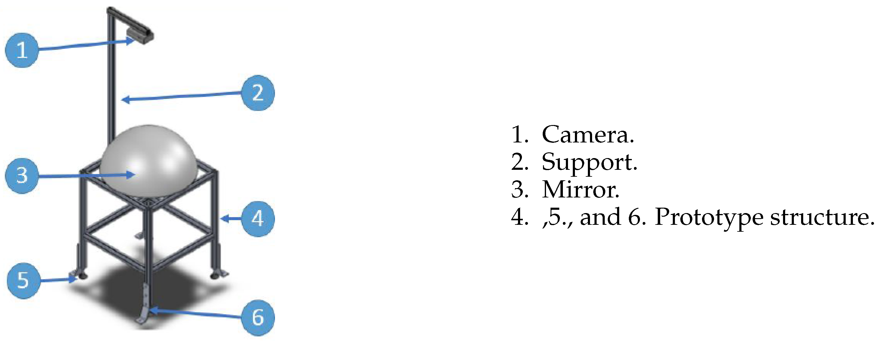
2.1. System Design
2.2. Sun Detection
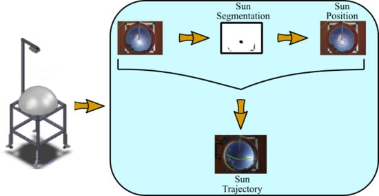
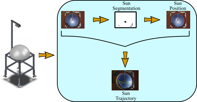
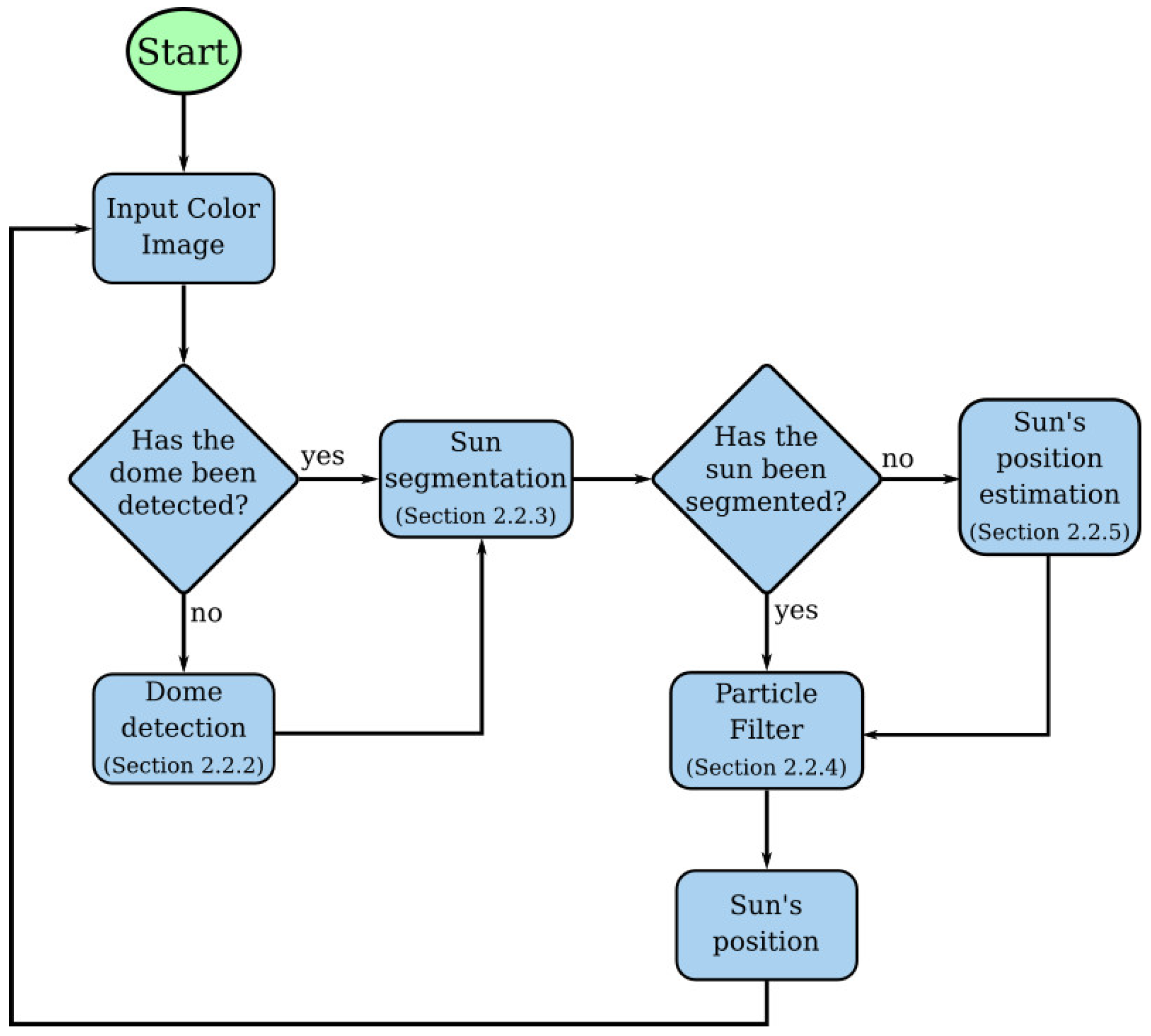
2.2.1. Framework
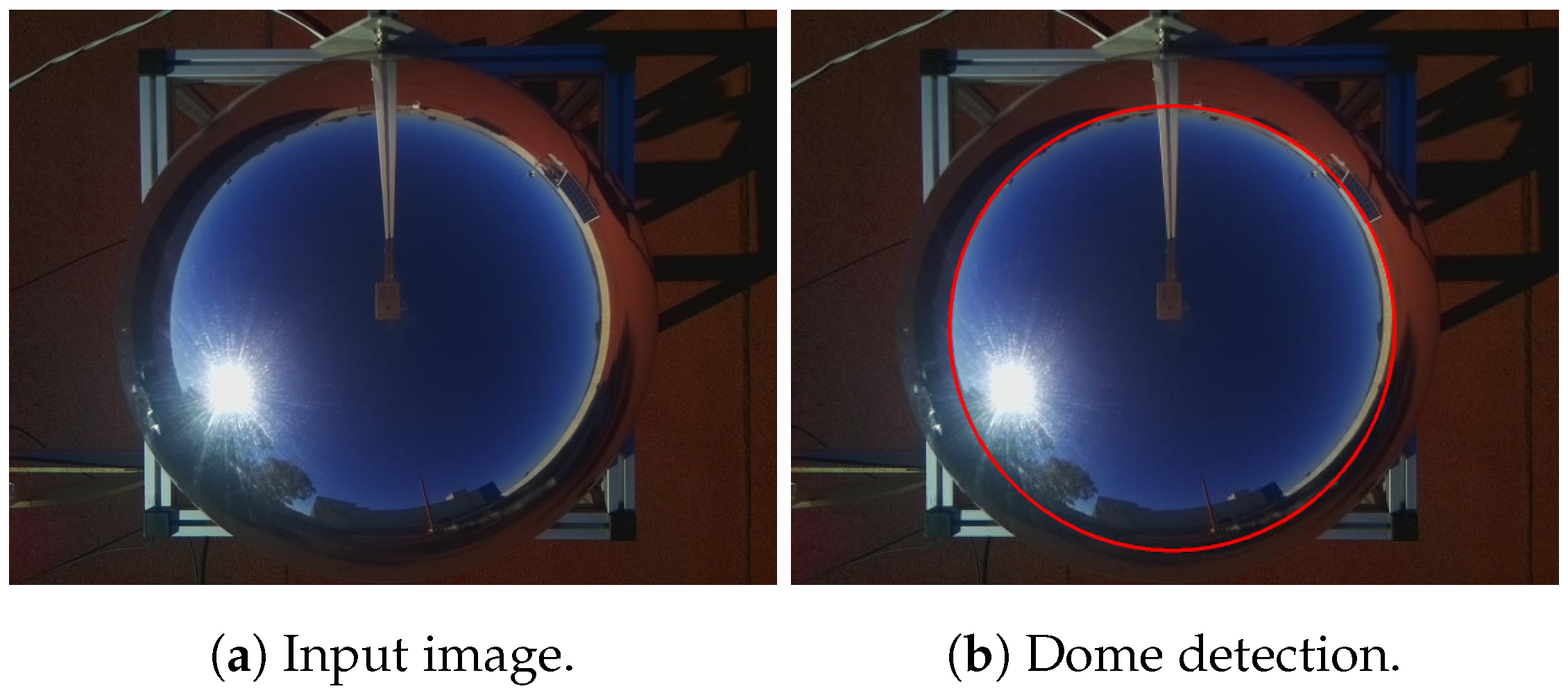
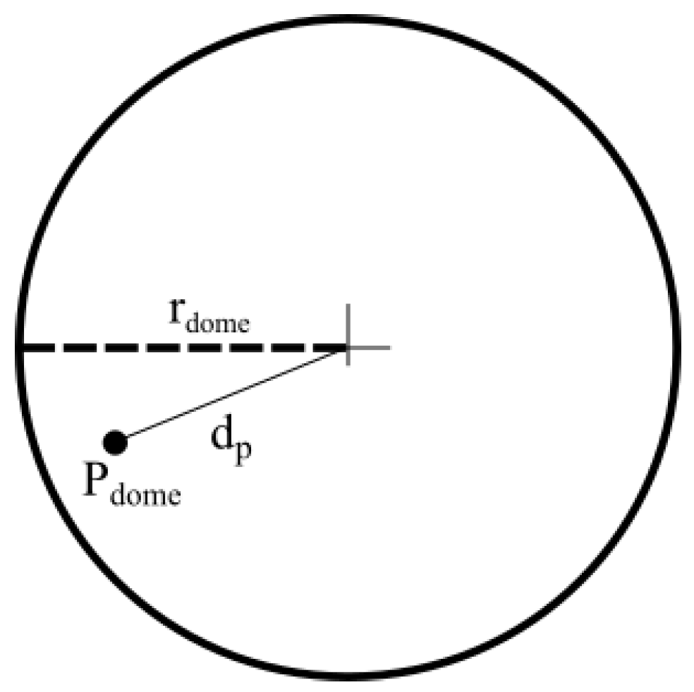
2.2.2. Dome Detection
| Algorithm 1 Dome detection algorithm. |
|
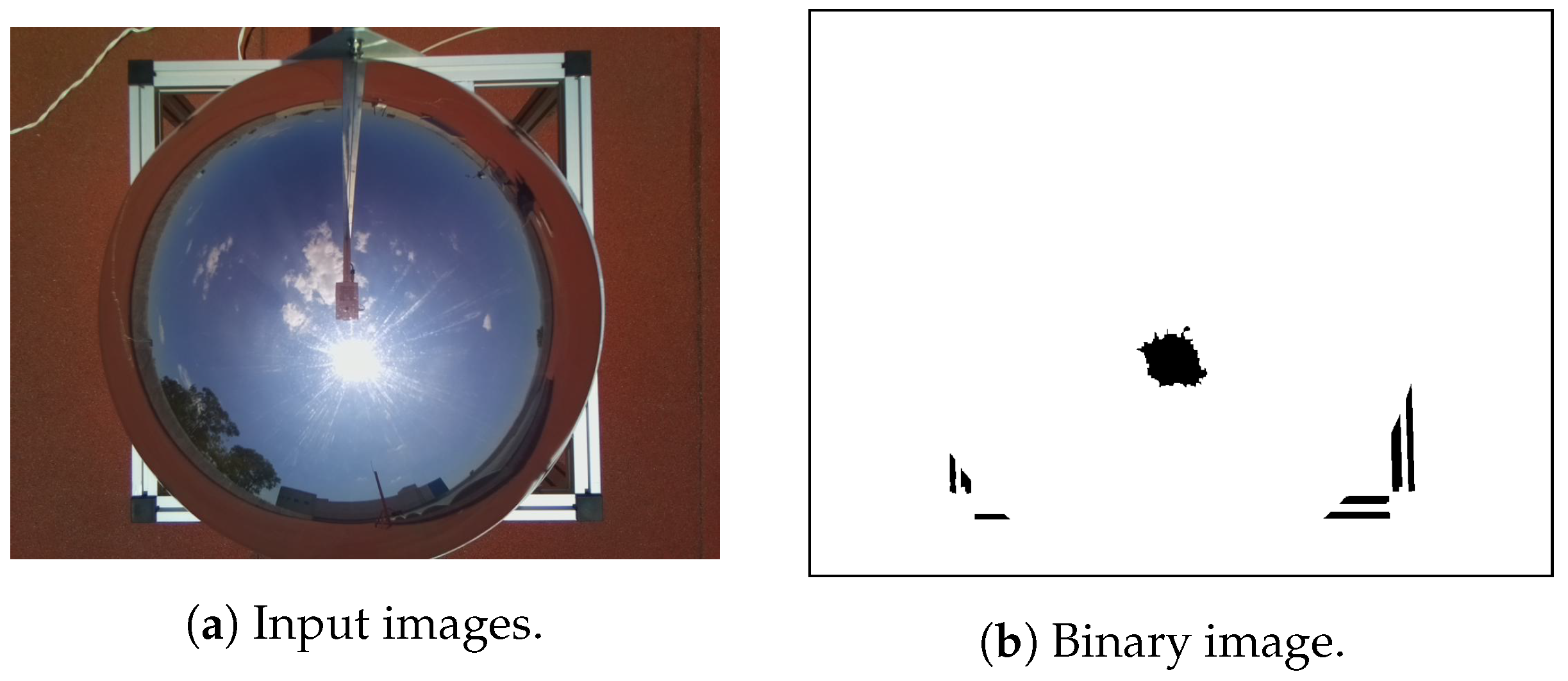
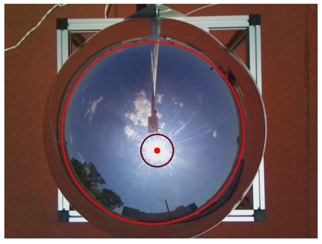
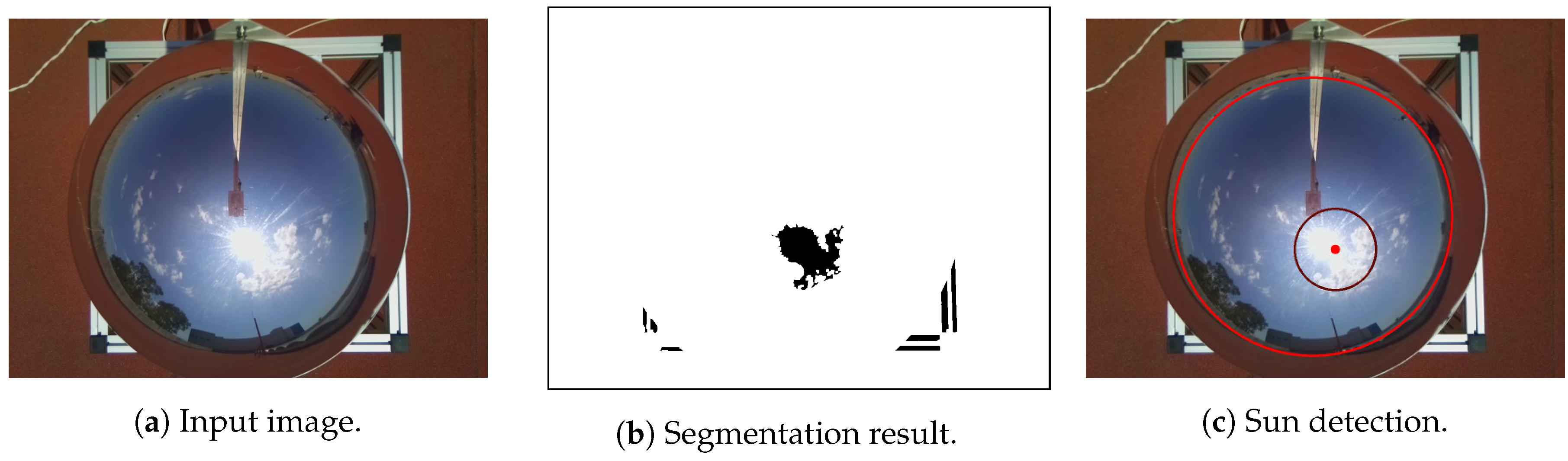
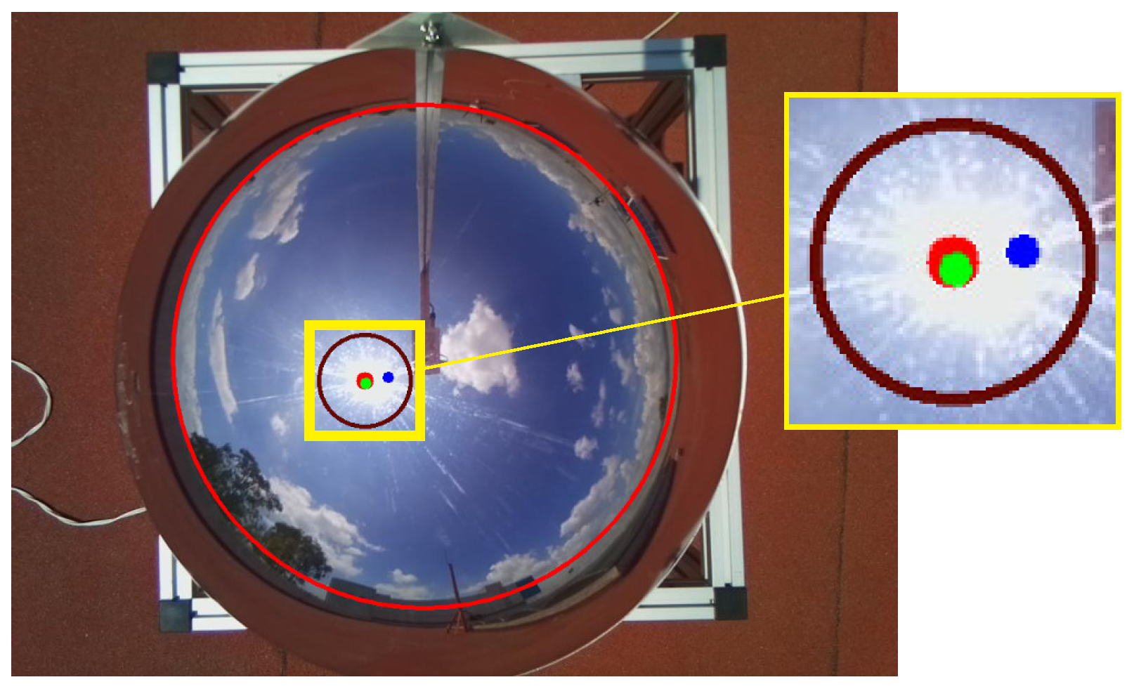
2.2.3. Clear Sky Sun Segmentation
| Algorithm 2 Sun-searching algorithm. |
|
2.2.4. Partially Sunny Day
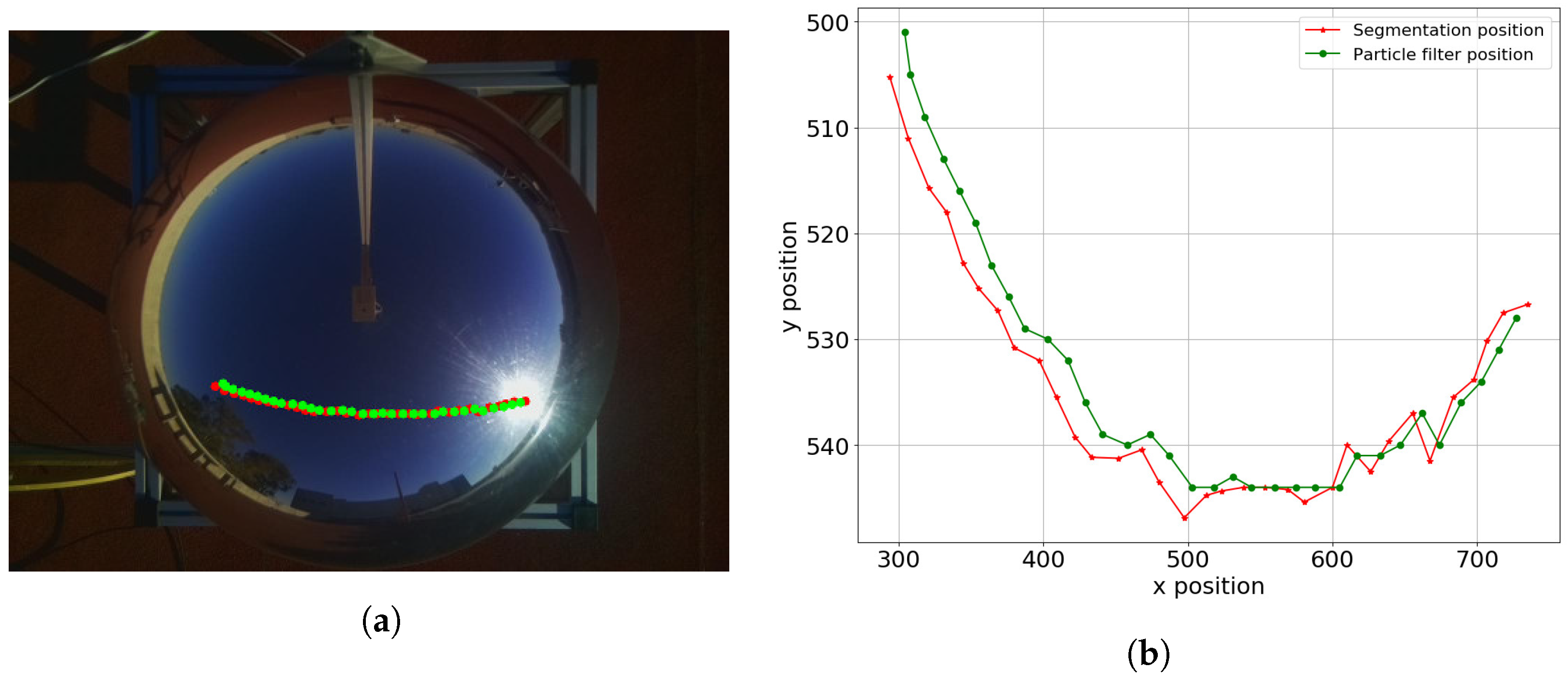
Particle Filter
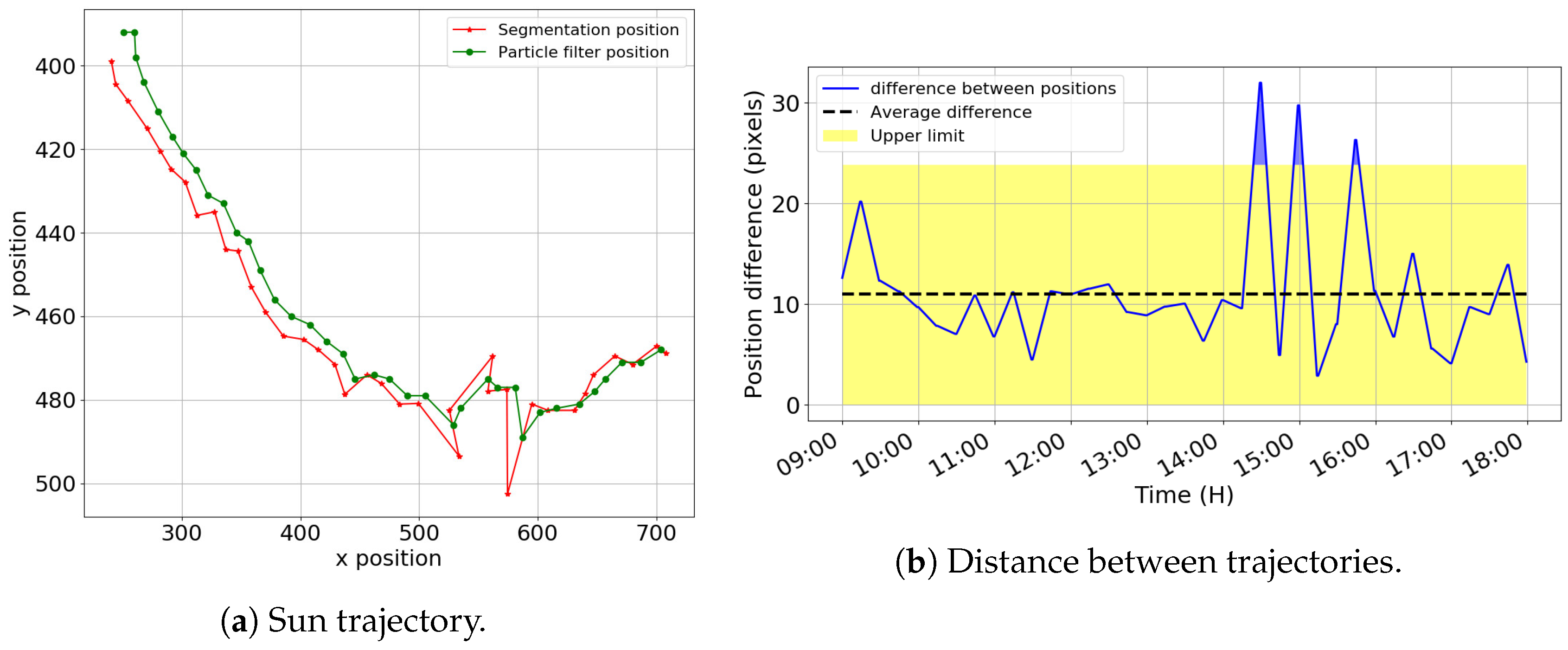
Sun’s Position Based on the Particle Filter
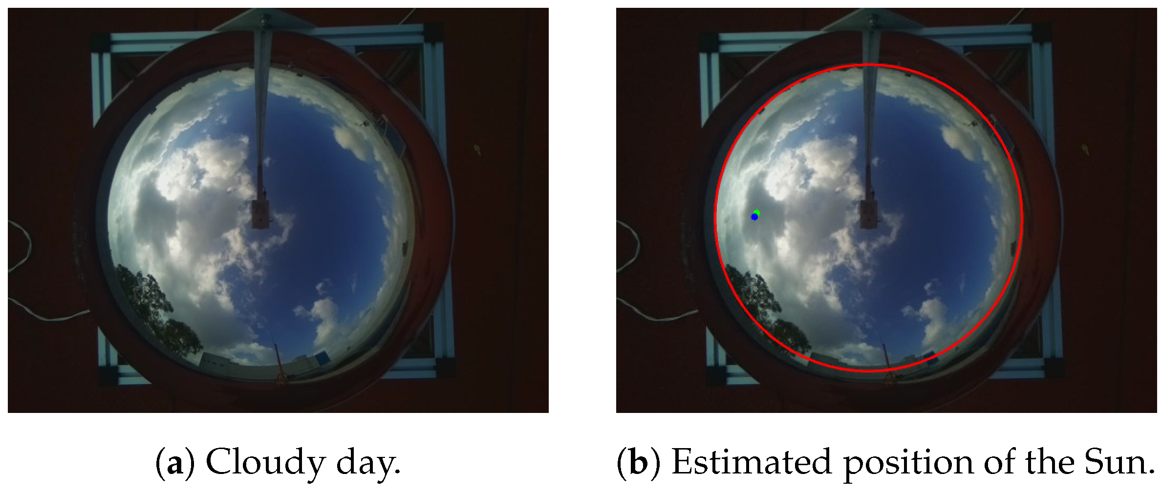
2.2.5. Detection of the Sun on Cloudy Days
3. Results and Discussion
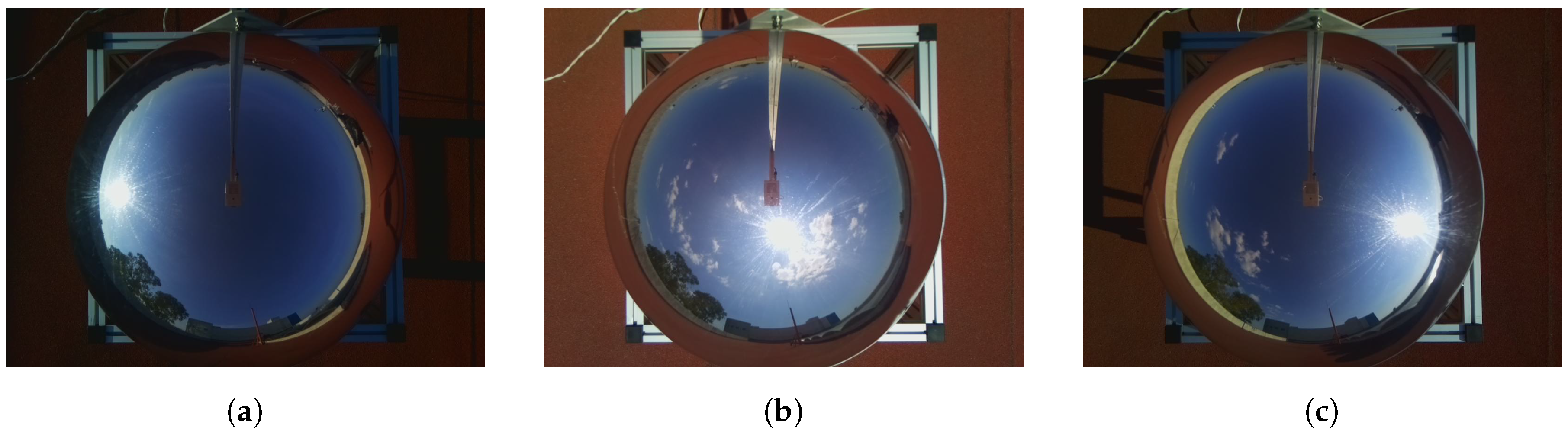
3.1. Scenario 1 (Sunny Day)
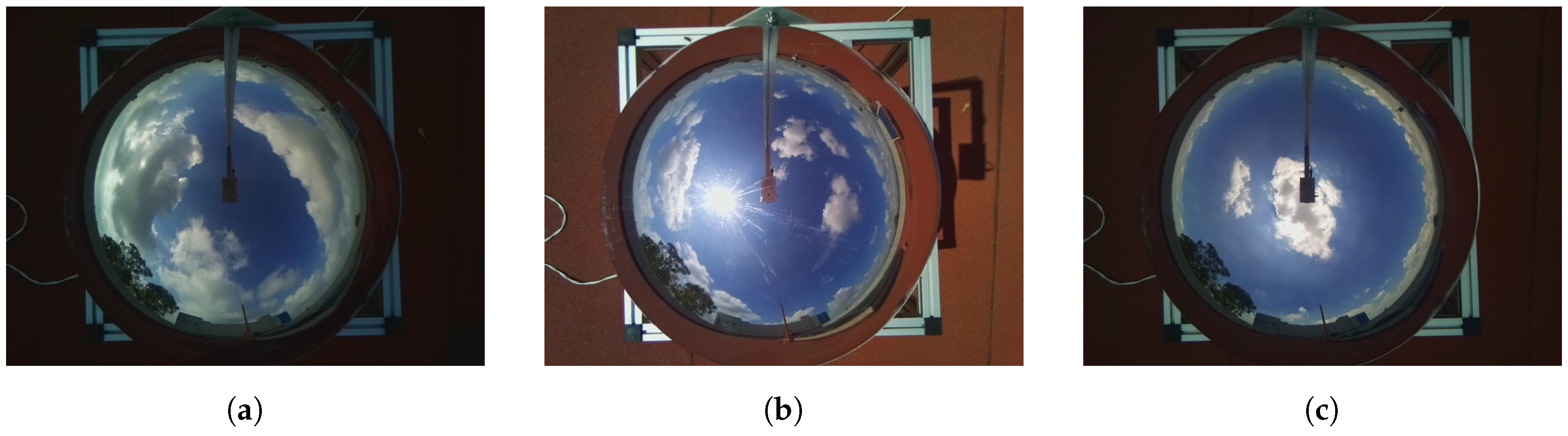
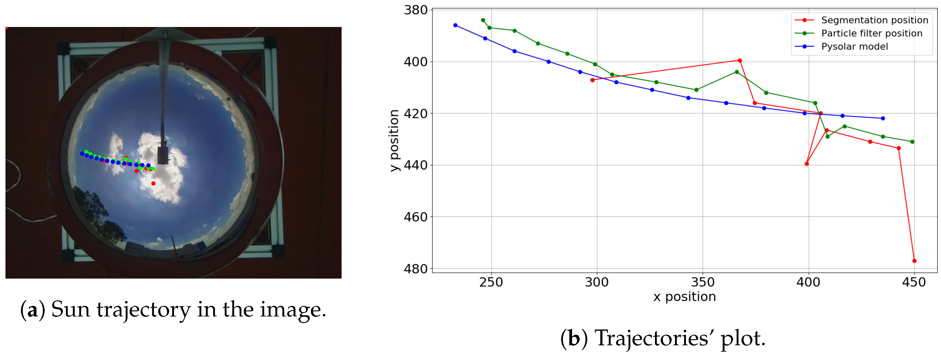
3.2. Scenario 2 (Partially Sunny Day)
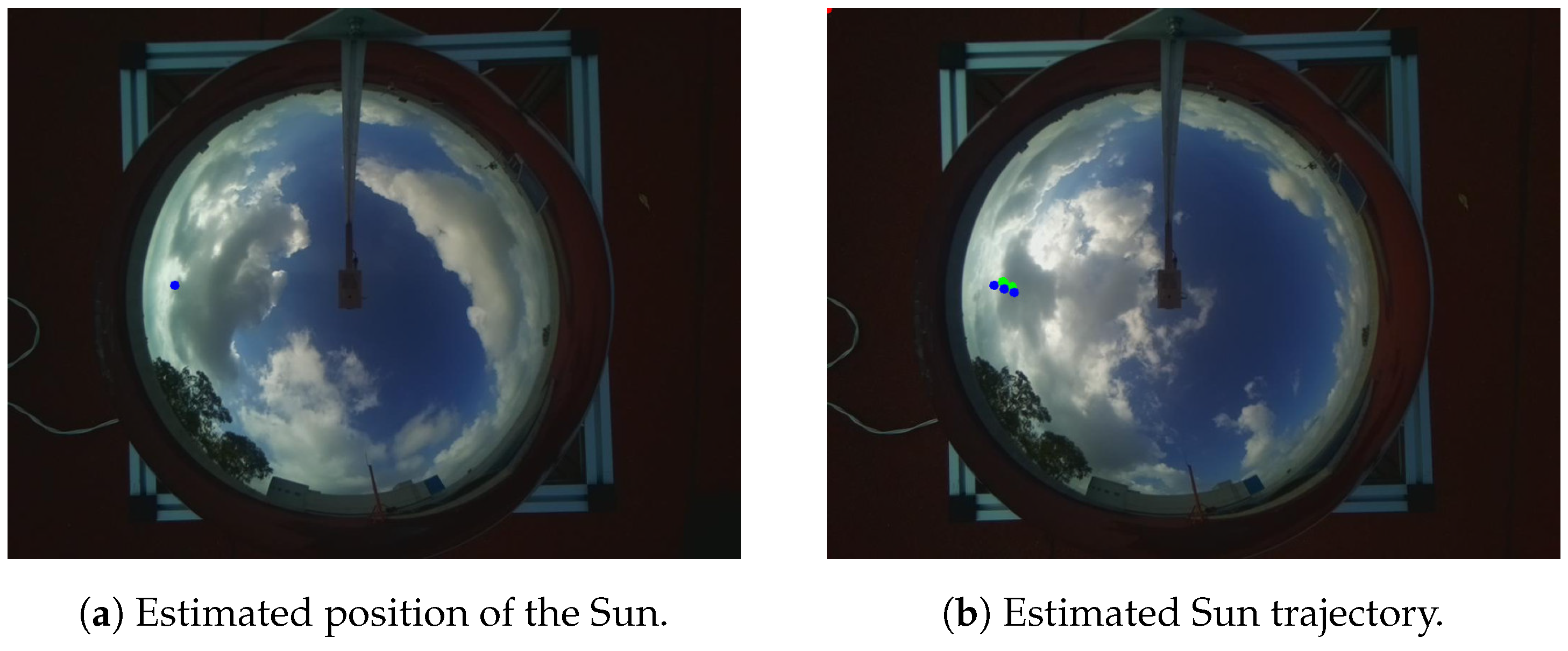
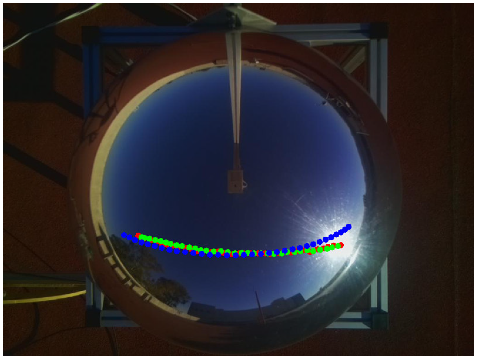
3.3. Scenario 3 (Cloudy Day)
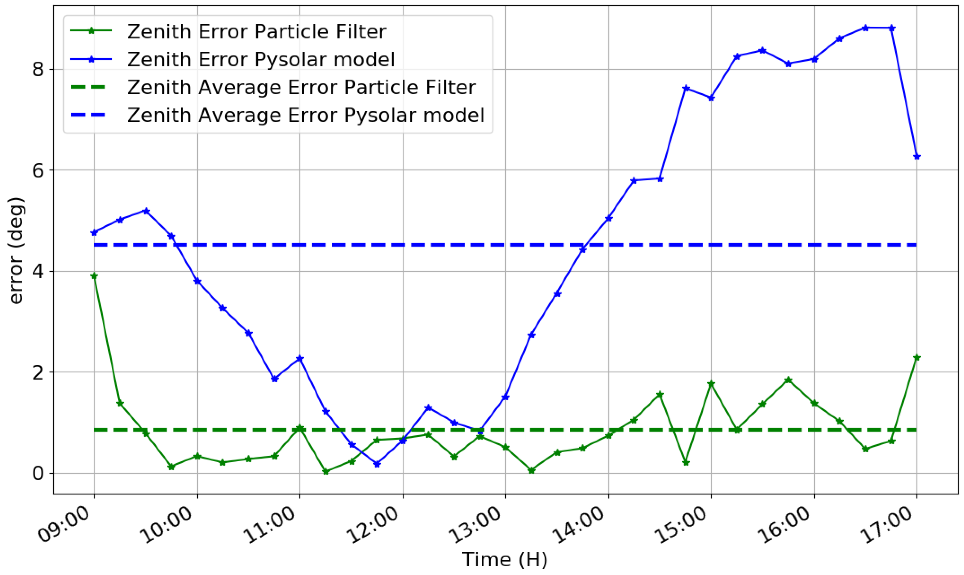
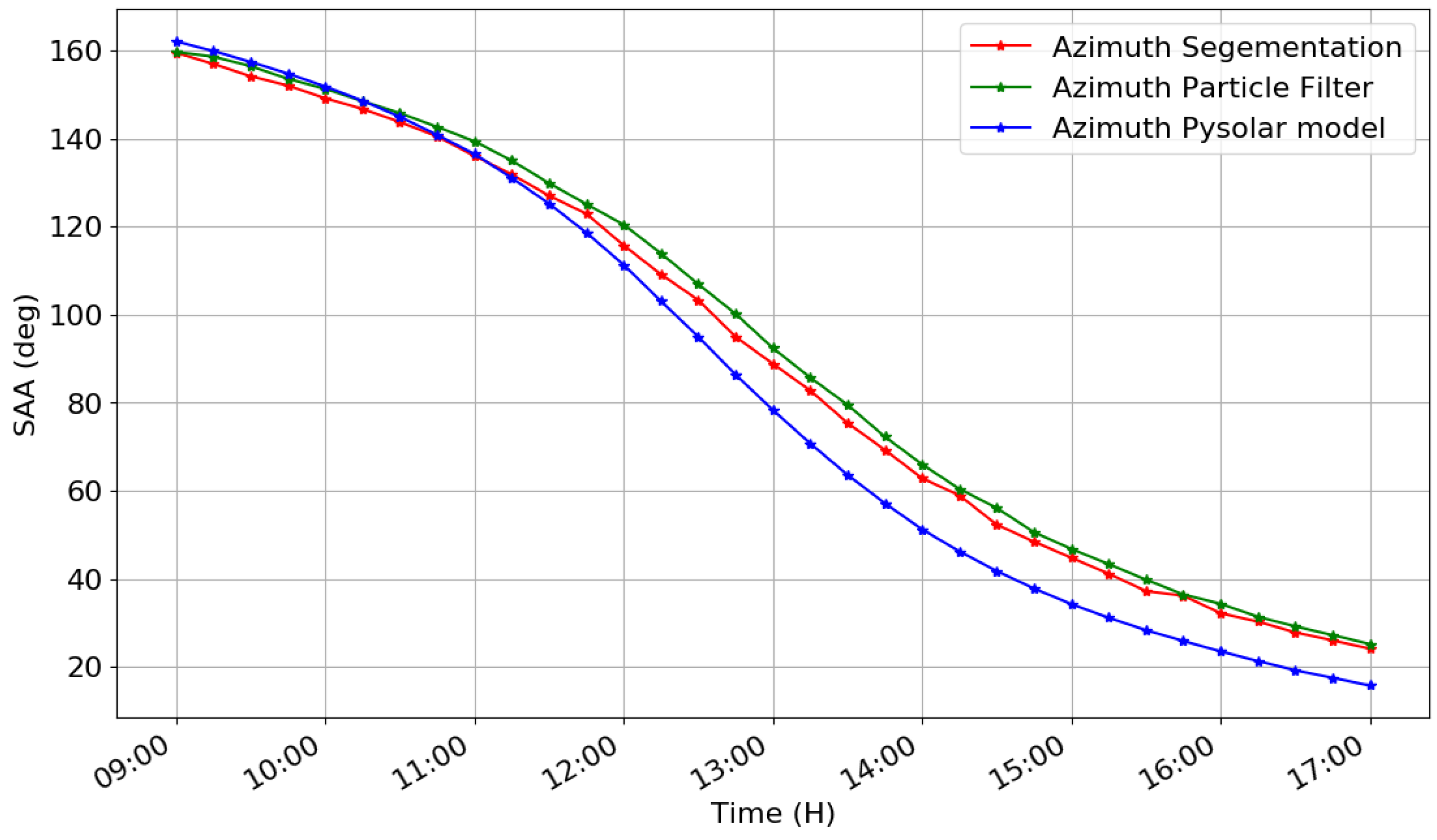
3.4. Detection Accuracy
4. Conclusions
Supplementary Materials
Author Contributions
Funding
Acknowledgments
Conflicts of Interest
References
- Chauvin, R.; Nou, J.; Thil, S.; Grieu, S. Modelling the clear-sky intensity distribution using a sky imager. Sol. Energy 2015, 119, 1–17. [Google Scholar] [CrossRef]
- Yang, H.; Kurtz, B.; Nguyen, D.; Urquhart, B.; Chow, C.W.; Ghonima, M.; Kleissl, J. Solar irradiance forecasting using a ground-based sky imager developed at UC San Diego. Sol. Energy 2014, 103, 502–524. [Google Scholar] [CrossRef]
- Long, C.N.; Sabburg, J.M.; Calbó, J.; Pagès, D. Retrieving Cloud Characteristics from Ground-Based Daytime Color All-Sky Images. J. Atmos. Ocean. Technol. 2006, 23, 633–652. [Google Scholar] [CrossRef] [Green Version]
- Meza, F.; Varas, E. Estimation of mean monthly solar global radiation as a function of temperature. Agric. For. Meteorol. 2000, 100, 231–241. [Google Scholar] [CrossRef]
- Valdes-Barrón, M.; Riveros-Rosas, D.; Arancibia-Bulnes, C.; Bonifaz, R. The Solar Resource Assessment in Mexico: State of the Art. Energy Procedia 2014, 57, 1299–1308. [Google Scholar] [CrossRef] [Green Version]
- Igawa, N.; Koga, Y.; Matsuzawa, T.; Nakamura, H. Models of sky radiance distribution and sky luminance distribution. Sol. Energy 2004, 77, 137–157. [Google Scholar] [CrossRef]
- Florita, A.; Hodge, B.; Orwig, K. Identifying Wind and Solar Ramping Events. In Proceedings of the 2013 IEEE Green Technologies Conference (GreenTech), Denver, CO, USA, 4–5 April 2013; pp. 147–152. [Google Scholar]
- Lorenz, E.; Kühnert, J.; Heinemann, D. Short Term Forecasting of Solar Irradiance by Combining Satellite Data and Numerical Weather Predictions. In Proceedings of the 27th European Photovoltaic Solar Energy Conference and Exhibition, Frankfurt, Germany, 24–28 September 2012; pp. 4401–4405. [Google Scholar]
- Chow, C.W.; Urquhart, B.; Lave, M.; Dominguez, A.; Kleissl, J.; Shields, J.; Washom, B. Intra-hour forecasting with a total sky imager at the UC San Diego solar energy testbed. Sol. Energy 2011, 85, 2881–2893. [Google Scholar] [CrossRef]
- Reikard, G. Predicting solar radiation at high resolutions: A comparison of time series forecasts. Sol. Energy 2009, 83, 342–349. [Google Scholar] [CrossRef]
- Marquez, R.; Coimbra, C.F. Forecasting of global and direct solar irradiance using stochastic learning methods, ground experiments and the NWS database. Sol. Energy 2011, 85, 746–756. [Google Scholar] [CrossRef]
- Chu, Y.; Pedro, H.T.; Li, M.; Coimbra, C.F. Real-time forecasting of solar irradiance ramps with smart image processing. Sol. Energy 2015, 114, 91–104. [Google Scholar] [CrossRef]
- Marquez, R.; Coimbra, C.F. Intra-hour DNI forecasting based on cloud tracking image analysis. Sol. Energy 2013, 91, 327–336. [Google Scholar] [CrossRef]
- Diagne, M.; David, M.; Lauret, P.; Boland, J.; Schmutz, N. Review of solar irradiance forecasting methods and a proposition for small-scale insular grids. Renew. Sustain. Energy Rev. 2013, 27, 65–76. [Google Scholar] [CrossRef]
- Kurtz, B.; Kleissl, J. Measuring diffuse, direct, and global irradiance using a sky imager. Sol. Energy 2017, 141, 311–322. [Google Scholar] [CrossRef]
- Nguyen, R.M.H.; Brown, M.S. Why You Should Forget Luminance Conversion and Do Something Better. In Proceedings of the 2017 IEEE Conference on Computer Vision and Pattern Recognition (CVPR), Honolulu, HI, USA, 21–26 July 2017; pp. 5920–5928. [Google Scholar]
- Deng, G.; Cahill, L.W. An adaptive Gaussian filter for noise reduction and edge detection. In Proceedings of the 1993 IEEE Conference Record Nuclear Science Symposium and Medical Imaging Conference, San Francisco, CA, USA, 31 October–6 November 1993; Volune 3, pp. 1615–1619. [Google Scholar]
- Bradley, D.; Roth, G. Adaptive Thresholding using the Integral Image. J. Graph. Tools 2007, 12, 13–21. [Google Scholar] [CrossRef]
- Almeida, A.; Almeida, J.; Araujo, R. Real-Time Tracking of Moving Objects Using Particle Filters. In Proceedings of the IEEE International Symposium on Industrial Electronics, ISIE 2005, Dubrovnik, Croatia, 20–23 June 2005; Volume 4, pp. 1327–1332. [Google Scholar]
- Nummiaro, K.; Koller-Meier, E.; Gool, L.V. An adaptive color-based particle filter. Image Vis. Comput. 2003, 21, 99–110. [Google Scholar] [CrossRef] [Green Version]
- Arulampalam, M.S.; Maskell, S.; Gordon, N.; Clapp, T. A tutorial on particle filters for online nonlinear/non-Gaussian Bayesian tracking. IEEE Trans. Signal Process. 2002, 50, 174–188. [Google Scholar] [CrossRef] [Green Version]
- Reda, I.; Andreas, A. Solar position algorithm for solar radiation applications. Sol. Energy 2004, 76, 577–589. [Google Scholar] [CrossRef]


© 2019 by the authors. Licensee MDPI, Basel, Switzerland. This article is an open access article distributed under the terms and conditions of the Creative Commons Attribution (CC BY) license (http://creativecommons.org/licenses/by/4.0/).
Share and Cite
Valentín, L.; Peña-Cruz, M.I.; Moctezuma, D.; Peña-Martínez, C.M.; Pineda-Arellano, C.A.; Díaz-Ponce, A. Towards the Development of a Low-Cost Irradiance Nowcasting Sky Imager. Appl. Sci. 2019, 9, 1131. https://doi.org/10.3390/app9061131
Valentín L, Peña-Cruz MI, Moctezuma D, Peña-Martínez CM, Pineda-Arellano CA, Díaz-Ponce A. Towards the Development of a Low-Cost Irradiance Nowcasting Sky Imager. Applied Sciences. 2019; 9(6):1131. https://doi.org/10.3390/app9061131
Chicago/Turabian StyleValentín, Luis, Manuel I. Peña-Cruz, Daniela Moctezuma, Cesar M. Peña-Martínez, Carlos A. Pineda-Arellano, and Arturo Díaz-Ponce. 2019. "Towards the Development of a Low-Cost Irradiance Nowcasting Sky Imager" Applied Sciences 9, no. 6: 1131. https://doi.org/10.3390/app9061131
APA StyleValentín, L., Peña-Cruz, M. I., Moctezuma, D., Peña-Martínez, C. M., Pineda-Arellano, C. A., & Díaz-Ponce, A. (2019). Towards the Development of a Low-Cost Irradiance Nowcasting Sky Imager. Applied Sciences, 9(6), 1131. https://doi.org/10.3390/app9061131