Validation of All-Sky Imager Technology and Solar Irradiance Forecasting at Three Locations: NREL, San Antonio, Texas, and the Canary Islands, Spain

Featured Application

Validation of all-sky imager technology at 3 locations: NREL, Joint Base San Antonio, and the Canary Islands, Spain.

Abstract

Increasing photovoltaic (PV) generation in the world’s power grid necessitates accurate solar irradiance forecasts to ensure grid stability and reliability. The University of Texas at San Antonio (UTSA) SkyImager was designed as a low cost, edge computing, all-sky imager that provides intra-hour irradiance forecasts. The SkyImager utilizes a single board computer and high-resolution camera with a fisheye lens housed in an all-weather enclosure. General Purpose IO pins allow external sensors to be connected, a unique aspect is the use of only open source software. Code for the SkyImager is written in Python and calls libraries such as OpenCV, Scikit-Learn, SQLite, and Mosquito. The SkyImager was first deployed in 2015 at the National Renewable Energy Laboratory (NREL) as part of the DOE INTEGRATE project. This effort aggregated renewable resources and loads into microgrids which were then controlled by an Energy Management System using the OpenFMB Reference Architecture. In 2016 a second SkyImager was installed at the CPS Energy microgrid at Joint Base San Antonio. As part of a collaborative effort between CPS Energy, UT San Antonio, ENDESA, and Universidad de La Laguna, two SkyImagers have also been deployed in the Canary Islands that utilize stereoscopic images to determine cloud heights. Deployments at three geographically diverse locations not only provided large amounts of image data, but also operational experience under very different climatic conditions. This resulted in improvements/additions to the original design: weatherproofing techniques, environmental sensors, maintenance schedules, optimal deployment locations, OpenFMB protocols, and offloading data to the cloud. Originally, optical flow followed by ray-tracing was used to predict cumulus cloud shadows. The latter problem is ill-posed and was replaced by a machine learning strategy with impressive results. R² values for the multi-layer perceptron of 0.95 for 5 moderately cloudy days and 1.00 for 5 clear sky days validate using images to determine irradiance. The SkyImager in a distributed environment with cloud-computing will be an integral part of the command and control for today’s SmartGrid and Internet of Things.

1. Introduction

The Department of Energy (DOE) estimates that PV power will grow to 14% of the electricity supply by 2030 as the price of solar electricity reaches a point at which it is cost-competitive with cogen ($0.06/kwh by 2020). It is imperative that power grid reliability and stability be maintained under this high penetration of low carbon energy [1]. Organizations such as North American Electric Reliability Corporation (NERC) and California Energy Commission (CEC) [2] have formulated several requirements needed in a “grid-friendly” PV power plant. For instance, CEC has developed a set of several smart inverter functionalities such as dynamic volt/var operation and ramp rate control. Existing PV plants do not have these functionalities even though the inverters are capable, due to the lack of communications standards and dynamic control. For PV power plants to participate in energy markets and ancillary services markets, they need to be considered “dispatchable” power plants.

High penetration of PV systems can be achieved if PV inverters [3] participate in the grid frequency regulation by active power control. Currently, frequency disturbances in the grid are handled by load curtailment. The disadvantage of this methodology is that it can cause voltage stress on the distributed generation. The alternative is to operate the PV system below its MPP (Maximum Power Point) to provide active power control. This can be done by modifying the MPP algorithm in such a way that it can track the next MPP point while working in the reduced power mode (RPM). A critical component of coordinated inverter control is forecasted solar power output or forecasted MPP at the array level. Having accurate intra-hour solar forecasts can enable implementation of a coordinated inverter control strategy capable of regulating a set-point, which may be a signal from a utility requiring either power curtailment or frequency regulation. The electric utility industry has yet to see an integrated solution to the dispatchability problem of PV plants, a system solution that effectively integrates intra-hour solar forecasting and smart control of inverters to achieve not only a grid-friendly plant, but also one that provides monetary and efficiency benefits to the PV plant operator.

Microgrids lack the stabilizing effects present in a large urban macrogrid that itself is joined to an interconnect; these issues are critical when a microgrid is operated in islanded mode. The Energy Management Systems (EMS) that balance PV output, load, and battery storage require accurate intra-hour irradiance forecasts to solve the control problem by shedding non-critical load when power generated is predicted to drop significantly below the load. An increasingly important problem for utilities is optimal scheduling and dispatch of a microgrid [4,5,6,7], both when connected to the macrogrid and when operated as an island. This task is divided into Day-Ahead Scheduling, which finds optimal schedules for the next operating day and focuses on energy markets, and Intra-day Dispatching and Scheduling in which schedules are continuously updated during the current day. Both cases follow these steps: (1) forecast day-ahead load, (2) forecast day-ahead renewable power (solar, wind), (3) Micro-Grid Management System (MGMS) optimizes the day-ahead plan, produces schedules for flows within the microgrid and to the PCC, (4) MGMS transmits schedules to utility control center.

This article describes a four-year research effort to develop hardware and software with an aim to solve the intra-hour solar forecasting problem for electric utilities. It was a collaborative effort between many groups, including national labs and research institutes (NREL and the Texas Sustainable Energy Research Institute TSERI), two universities (The University of Texas at San Antonio and Universidad de La Laguna in the Canary Islands), public and private utilities (CPS Energy, ENDESA, and Duke Energy), and a private company, Siemens-Omnetric. It serves as a case study in managing research in a joint theatre of operations and integrating the efforts of researchers and engineers who came from very different university and industrial cultures. Details of our research and technology development have been presented in journal articles [8,9], conference proceedings [10,11,12,13], and technical reports [14]. While this paper gives a detailed overview of that research, our primary goal is to describe how the UTSA SkyImager was validated at three geographically diverse locations, the pitfalls encountered, the lessons learned, and the outlook for future research efforts.

The SkyImager evolved from a realization that existing all-sky imaging systems were too expensive to be deployed in large numbers, suffered from data-loss issues caused by the shadow band and camera arm, and used proprietary software. The Raspberry Pi single board computer ($35) and programable high-resolution Pi-Cam ($20) with a fisheye lens ($20) formed the heart of the new system. The most expensive component was the all-weather security camera enclosure ($350). In addition, General Purpose IO (GPIO) pins would allow a variety of external sensors to be connected to the Pi. Low cost and ease of use were essential if the SkyImager were to be deployed in a rural sustainable development microgrid. In contrast to some commercial all-sky imaging systems, only open source software would be used. The Pi accommodates several operating systems (OS) including Raspbian, a Linux-based derivative of Debian. It can be operated with a monitor or in “headless” mode, and once deployed can be accessed remotely with SSH/SFTP. Code for the SkyImager would be written in Python and allow calls to libraries such as Open Computer Vision, Scikit-Learn, SQLite, and Mosquito. In the summer of 2014 it was an open question whether the proposed imager could deliver the functionality of much more expensive systems and be thoroughly tested before its deployment.

As part of the DOE microgrid INTEGRATE program, the first deployment of the SkyImager occurred in Fall 2015 at the ESIF building at NREL. INTEGRATE aggregated sustainable generation and loads into microgrids controlled by an Energy Management System with the OpenFMB protocol. In 2016 a second SkyImager was installed at the CPS Energy microgrid at Joint Base San Antonio. A multi-year collaboration between CPS-UTSA and the Universidad de La Laguna resulted in the deployment of two SkyImagers in the Canary Islands. These utilize stereoscopic images to determine heights of the bases of cumulus clouds. Deployment of SkyImagers in three diverse locations provided not only big data, but operational experience in harsh extremes of climate. This resulted in improvements and additions to our original design: weatherproofing, new environmental sensors, the need for scheduled maintenance, optimal positioning of the camera, communications with OpenFMB publish-subscribe protocols, and using WiFi and cloud computing. The SkyImager will be an integral part of the command and control for microgrids, both as part of the larger SmartGrid in an urban environment or in an islanded mode in a military or rural setting.

Solar forecasting is widely considered a key means of integrating solar power efficiently and reliably into the electric grid. For a utility to meet projected customer demand with electricity from sustainable resources, high-accuracy global horizontal irradiance (GHI) forecasts must be available over widely different time and space scales. A convenient separation of this forecasting problem into two parts is as follows: (1) intra-hour forecasts of the ramp events that are caused when cumulus clouds move between the sun and the solar panels, and (2) day-ahead forecasts for 12, 24, and perhaps 36 h into the future. There is overlap between the two parts, but this taxonomy is convenient not only because the physics and forecasting techniques are generally different, but also the way in which the utility makes use of the forecasts. A single ramp event on a microgrid powered primarily by PV arrays can result in over/under voltages, as well as frequency deviations and may require secondary spinning reserves to be brought on line. Day-ahead irradiance forecasts are useful in predicting surplus/deficit generation capacity that can then be augmented or sold in the day-ahead electricity market.

1.1. Day-Ahead GHI Forecasting

For day-ahead GHI forecasting, both numerical weather prediction (NWP) [15] and satellite imagery provide effective tools for forecasting irradiance. The National Center for Environmental Prediction (NCEP), a part of NOAA, runs two versions of the Rapid Refresh (RAP) numerical weather model to predict environmental data. The first version generates weather data on a 13-km (8-mile) resolution horizontal grid and the second, the High-Resolution Rapid Refresh (HRRR), generates data on a 3-km (2-mile) grid. RAP forecasts use multiple data sources: commercial aircraft weather data, balloon data, radar data, surface observations, and satellite data to generate forecasts with hourly resolution in time and forecast lengths of 18 hours. For further details, consult the RAP website [16]. RAP data are available for download through the National Model Archive and Distribution System (NOMADS). Several benefits accrue from using NWP for irradiance forecasting: NOAA incurs much of the computational burden and these models incorporate first-principles physics such as the Navier-Stokes equations, thereby allowing for the dynamic formation of clouds. Satellite technology is advancing rapidly with GOES-16 (Geostationary Operational Environmental Satellite) pictures being updated every 5 min with maximum resolution of 5000 by 3000 pixels. Figure 1 shows such an image cropped to the central Texas region. The temporal sampling of the data is still insufficient to support optical flow predictions 15-min ahead. Continued improvements in GOES-R (geostationary satellite with high spatial and temporal resolution) may well make the satellite approach to minutes-ahead irradiance prediction more attractive in the future [17,18,19,20]. Statistical methods based on historical time-series data and climatology are also useful for day-ahead PV forecasting.

1.2. Intra-Hour Solar Forecasting

The energy alliance between UTSA and CPS Energy has as one of its primary goals the development of new solar forecasting technologies that combine inexpensive all-sky imaging cameras with sophisticated image processing techniques and artificial intelligence software to produce high-accuracy 15-min ahead solar irradiance forecasts. GHI consists of two components, the Direct Normal Irradiance (DNI) caused by sunlight traveling in a direct path from sun to PV array and the Diffuse Horizontal Irradiance (DHI), background illumination that is due to secondary reflections and absorption/re-radiation. The formula is GHI = cos(θ_z) DNI + DHI where θ_z is the zenith angle. Shadows cast by low-level cumulus clouds significantly impact the DNI but have little effect upon the background DHI. While it is possible to predict DNI separately [21], for verifying PV power output forecasts GHI is used. Figure 2 displays the three quantities: GHI, DNI, and DHI, on the date 27 October 2015 at the NREL ESIF facility in Golden, CO. It shows that moderately cloudy conditions occasion multiple ramp events.

Figure 3 displays a sequence of eight pictures taken by the SkyImager at the NREL site, one every two minutes starting (upper left) at 12:31pm MST. At that time the sun is not obscured, but cumulus clouds are moving in from the left. At 12:35 the cloud begins to enter the solar disk and by 12:37 the sun is completely occluded. This continues until 12:44 when the cloud has moved past the sun and the DNI recovers. This ramp event is seen in the DNI oscillations that occur around the noon hour in Figure 2. While this example considers a single ramp event, it strongly suggests that the correlation between measured GHI and the presence of clouds obscuring the sun in the SkyImager pictures could be learned by AI models.

The challenge in short term prediction of PV power is simply “Where will cumulus cloud shadows be fifteen minutes from now?” Our approach incorporates as much of the physics as possible, but is an idealization necessitated by the requirement to produce GHI forecasts in real time for the MGMS. Solving Navier-Stokes for the true dynamics of the atmosphere is not feasible on a Raspberry Pi. If GHI can be accurately forecast, then predicting PV power output is straightforward. The evolution of clouds and irradiance shown in Figure 2 and Figure 3 is even more striking when video of the images is viewed, confirming that SkyImager pictures are highly correlated with the observed GHI time series. Moreover, it suggests the camera sensor could be used to measure irradiance as well as predict it. Once GHI has been accurately forecast, it is usually straightforward to assign a corresponding PV power output, which is what the MGMS requires.

Figure 4 shows the relationship between GHI (Watts/m²) and PV power (Watts) from the RSF2 PV arrays located at NREL. The relationship is almost linear with a slight hysteresis effect that reflects the differences in morning versus afternoon irradiance. The task of predicting PV power output over multiple temporal and spatial scales, and from a variety of different equipment is a challenging one [22,23,24].

State of the Art in Solar Forecasting

As photovoltaics achieve greater penetration, the SmartGrid will demand accurate solar forecasting hence a network of low cost, distributed sensors to acquire large amounts of image and weather data for input to the forecasting algorithms. Commercial sky imaging systems often prove too costly and have proprietary software, leading several research groups to develop their own systems. The solar forecasting research group at UC San Diego [25,26,27,28,29] has done pioneering work in this field for many years. For one example, Coimbra et al. [30] proposed DNI forecasting models using images from a Yankee TSI 880 with hemispherical mirror as inputs to Artificial Neural Networks (ANN). The TSI has high capital and maintenance costs, uses a shadow band mechanism, and requires proprietary software. The UCSD Sky Imager described in Yang et al. [31] captures images with an upward-facing charge-coupled device (CCD) Panasonic sensor and a 4.5 mm focal length fisheye lens. Compared with the TSI it has higher resolution, greater dynamic range, and lossless PNG compression. The Universitat Erlangen-Nurnberg [32] group used a five-megapixel C-mount camera equipped with a fisheye lens. They implemented the Thirions ”‘daemons’” algorithm for image registration and cloud-motion estimation similar to optical flow. In Australia, West et al. [33] used off-the-shelf IP security cameras (Mobotix Q24, Vivotek FE8172V) for all-sky imaging. Inexpensive compared to the TSI, the cost of such systems still is ~800 euros. Rather than a feature-tracking strategy, they used dense optical flow to estimate cloud movement. See also Wood-Bradley [34]. Several research groups in China are working on the irradiance forecasting problem [35,36] generally using a TSI imager, but in one case Geostationary Statellite data [37]. As mentioned before dramatic improvements in GOES-R technology and resolution (spatial and temporal) will make this approach more attractive for intra-hour forecasting. See also the historical review [38] of irradiance and PV power forecasting that was produced using text mining and machine learning.

A recurring theme in the INTEGRATE project was that while all-sky imaging was a critical component of microgrid stability and control, it could not be developed in a stand-alone fashion but must be fully integrated into the microgrid management system (MGMS). Uriate et al. [39] discuss the importance of Ramp Rates (RR) on the inertial stability margin of a microgrid deployed at the Marine Corp Base at Twentynine Palms. They show that a large ramp in PV power can destabilize frequency when the PV load is suddenly transferred to the cogen. The inertia constant H of a generator is the ratio of stored kinetic energy to system capacity. Microgrids usually have H < 1 s compared to 2–10 s for large generation plants. Frequency stability is defined by the condition $\left|\Delta f_{pu}\right|<\Delta f_{max}^{pu}$ where allowable frequency deviation $\Delta f_{max}^{pu}$ in p.u. is typically 0.01–0.05 per unit. In [39] the authors derive the ODE ${\mathsf{\omega }}_{mech}{\mathrm{Jd}\mathsf{\omega }}_{mech}/\mathrm{dt}+{\mathsf{\omega }}_{mech}^2\mathrm{D}=P_{accel}$ where ${\mathsf{\omega }}_{mech}$ is the mechanical speed of the generator in rad/s, J the moment of inertia (kg∙m²), D a damping coefficient (Nm/s), and P_accel the power imbalance exerted on a generator rotor, to model the microgrid stability control problem. The NREL microgrid has a 300 kW Caterpillar diesel generator, whereas JBSA has no cogen. However, the same issues of stability and frequency control apply when there are no spinning resources. Some electric codes are specifying ancillary control must be added to the EMS in order to handle ramp events of a certain magnitude and duration. See [40,41,42] for details.

1.3. Climatology and Microgrid Architectures at the Three Locations

As shown in Figure 5 the UTSA SkyImager has been deployed at 3 geographically diverse locations: Golden, Colorado on the rooftop of the ESIF building at NREL, in San Antonio, Texas at the CPS Energy microgrid facility at Joint Base San Antonio (JBSA) and the Engineering Building at UTSA, as well as in the Canary Islands, Spain at Tenerife and Caleta de Sebo. Each location presented unique challenges in terms of local climate, physical and cyber access, and microgrid design, equipment, operation, and customer needs.

The UTSA SkyImager was first conceived as a technology for providing accurate intra-hour irradiance forecasts as inputs to a microgrid management system that would then provide the utility with command and control of the microgrid in either connected or islanded mode. The Department of Energy INTEGRATE project [43] lasted for 18 months beginning on 6 March 2015 and partnered NREL, Omnetric-Siemens, CPS Energy, Duke Energy, and UTSA. The project goal was to increase the capacity of the electric grid to incorporate renewables by upgrading and optimizing architectures for control and communication in microgrids. There were three major components: (1) OpenFMB, a reference architecture that allows real time interaction among distributed intelligent nodes, (2) optimization with the Spectrum Power Microgrid Management System based on the Siemens SP7 Platform, and (3) PV and Load Forecasting using UTSA’s applications for both intra-hour and day-ahead irradiance and building load forecasts. The OpenFMB framework leverages existing standards such as IEC’s Common Information Model (CIM) semantic data model and the Internet of Things (IoT) publish/subscribe protocols (DDS, MQTT, and AMQP) to allow flexible integration of renewable energy and storage into the existing electric grid. The OpenFMB standard was ratified by the North American Energy Standards Board (NAESB) in March of 2016 and allows communication between diverse grid devices–meters, relays, inverters, capacitor bank controllers, etc. It allows federated message exchanges with readings such as kW, kVAR, V, I, frequency, phase, and State of Charge (SOC) published every 2 seconds as well as data-driven events, alarms, and control in near-real-time.

1.3.1 SkyImager at National Renewable Energy Laboratory in Golden, CO

The site of the first SkyImager deployment was NREL in the Rocky Mountains. Golden’s high elevation and mid-latitude interior continent geography results in a cool, dry climate. There are large seasonal and diurnal swings in temperature. At night, temperatures drop quickly and freezing temperatures are possible in some mountain locations year-round. The thin atmosphere allows for greater penetration of solar radiation. As a result of Colorado’s distance from major sources of moisture (Pacific Ocean, Gulf of Mexico), precipitation is generally light in lower elevations.

Eastward-moving storms from the Pacific lose much of their moisture falling as rain or snow on the mountaintops. Eastern slopes receive relatively little rainfall, particularly in mid-winter. The SkyImager enclosure came equipped with a heater/fan that performed well at NREL. Given the climate, it proved useful in keeping frost off the plastic dome. It adds to the expense and complexity of the technology and may not be required at other locations. Most installations of the security camera enclosure would be facing downward and perhaps under a building overhang. Used facing upward and exposed to the sky, there were issues with water getting inside the enclosure. A simple solution was silicon caulk applied at the base of the dome. In a typical security installation, a green tinted plastic dome is used with the enclosure to protect components from UV radiation. For all-sky imaging a clear plastic dome is a necessity. With any plastic material on a bright sunny day there can be issues with glare caused by the dome, but this was minor. The alternative is a glass dome but that has it own set of problems.

As shown in Figure 6, the microgrid at NREL was already well established and the process of deploying the SkyImager went relatively smoothly. Denver International Airport is located some 36 miles from Golden; this distance introduces some error in the Cloud Base Height for the ray-tracing algorithm originally used in the SkyImager. The ESIF building at NREL had the infrastructure necessary for easy installation of both the SkyImager and the Hardkernel Odroid C1 single board computer (SBC) used for load and day-ahead PV forecasts. Information was transferred using a Wi-Fi network on a LAN system. NREL also provided un-interruptible 120 VAC power, ample Ethernet connectivity, and excellent on-site weather and irradiance data. In addition to solar PV arrays, generation included a 500 kW wind power simulator and a 300 kW caterpillar diesel. A 300 kWh battery system provided energy storage and the load was separated into a controllable component (250 kW) and a critical load (250 kW).

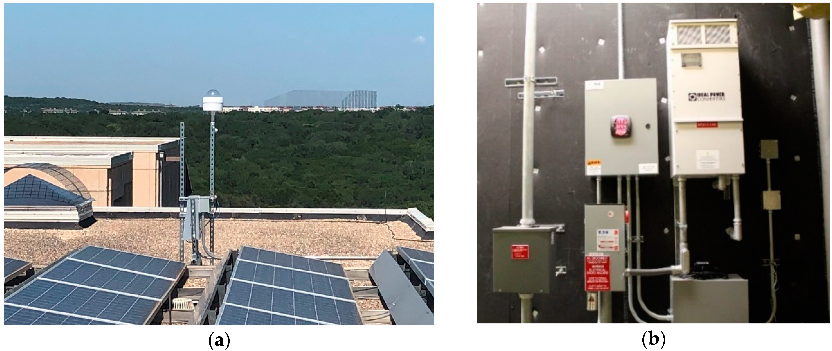
1.3.2. SkyImager at San Antonio, TX, USA

Texas produces more electricity than any of the other 49 states, and as a result has its own interconnect ERCOT. In 2017, power statewide was generated by a variety of sources: natural gas (45%), coal (30%), wind (15%), and nuclear (9%). In 2014, wind replaced nuclear as the third-largest source of power and Texas now produces more wind power than any other state. Solar generation is increasing, but still relatively small for a state with abundant annual sunshine. Located in central Texas some 200 miles from the Gulf of Mexico, San Antonio is home to almost 1.5 million people and several military bases. CPS Energy serves San Antonio and is the nation’s largest public power, natural gas and electric company. They are committed to renewables, funding a 400 MWac project with multiple PV plants (Alamo 1–7) close to San Antonio, and wind farms in West and South Texas. CPS Energy is among the top public power wind energy buyers in the nation and number one in Texas for solar generation. In keeping with this commitment, TSERI was formed in 2001 as an alliance between CPS Energy and UTSA.

For San Antonio, the most significant local weather issue is low-level Gulf stratus [44]. Elevations of the terrain increase from sea level at the Gulf coast to almost 800 ft at San Antonio, and a moist air mass over the Gulf of Mexico will cool adiabatically to saturation as it moves upslope. Nocturnal radiational cooling causes cloud formation before midnight, resulting in a ceiling of 500–1000 feet. A solid cloud deck will cover much of central Texas and remain in place until late morning when the sun burns off the stratus and cumulus clouds begin to form. Forecasting Gulf stratus is an important problem for aviation; it is a matter of accurately predicting low-level wind flow (<5000 ft) with the most favored wind direction for stratus formation from 90° to 180°. It is important to address these local weather conditions that occur below the spatial and temporal resolution of NWP, but are crucial for both inter-hour and day-ahead irradiance forecasts. Use of machine learning using local datasets and climatology will allow the information and intelligence of a study such as [44] to be incorporated in site-specific irradiance forecasts.

The Fort Sam Houston Library location at JBSA presented several unique challenges for the deployment of the UTSA hardware and software, challenges that provide valuable insights for other researchers. Many of the issues that arose were heavily dependent on the specific location. At JBSA, the Sky Imager was deployed using an edge-computing configuration with a wired Ethernet connection for cyber security. The JBSA microgrid is shown in Figure 7 and includes the Base Library building, solar arrays, inverters, and the pod housing the battery energy storage system (ESS). The need for accurate on-site meteorological observations necessitated installation of a complete MET Station atop a 10m antenna tower. A Campbell Scientific weatherproof instrument box at the tower base contained a National Instruments MyRio computer, a transformer, backup battery, and an Odroid C2 single board computer (SBC) for calculating the day-ahead load/PV forecasts. Atop the tower sat the SkyImager, a WXT520 Vaisala weather transmitter, and a pyranometer.

In July of 2018 another SkyImager was deployed in San Antonio at the location of a university PV generation project. Funded by a DOE-SECO grant [45] in 2014, solar panels were installed on the Engineering Building, HEB University Center III, and Durango buildings at UTSA. In addition, equipment was installed to record measurements from 4 Combiners, 4 Inverters, 2 Kipp & Zonen CMP11 pyranometers, and a WXT520 Vaisala Weather Transmitter at the UCIII. Figure 8a displays the SkyImager and PV panels and Figure 8b shows combiners/inverters atop the Engineering Building. The only ingredient lacking to make this a research microgrid was energy storage.

1.3.3. SkyImager in the Canary Islands

Six insular power grids comprise the electrical network in the Canary Islands. Conventional generation costs more here than PV technologies, and savings can be shared between the PV system owners and the Spanish utility ENDESA. Penetration of renewables varies among these grids, from a high of 60% penetration of wind energy in El Hierro (after Gorona del Viento hydro-wind power plant is operational) to Lanzarote-Fuerteventura which achieves single-digit integration of renewables because of strong environmental regulations, a weak power grid, and an unstable regulatory environment in Spain for renewable energy infrastructure during the period 2011-15. However, new regulatory policies will provide a more attractive framework for investment. The Canary Islands Government plans to avoid ground-based renewable facilities with a large environmental footprint in favor of smaller rooftop plants close to electricity users. As in Hawaii, the existing distribution grid is not prepared for a large penetration of residential PV systems with resulting reverse flows, voltage and frequency instabilities, and drops at the end of long lines. ENDESA has built a testbed smart grid in a village at the north end of the Fuerteventura-Lanzarote insular power system (La Graciosa).

La Graciosa is the smallest island in the Canary Archipelago with a surface area of 29 km². It is in a marine nature reserve north of Lanzarote and home to about 700 people in the island capital of Caleta de Sebo. Average global irradiation is 5.157 kWh/ kW·day (1883 kWh/kW·yr) while the average monthly high temperature is 20.8 °C. Located a few kilometers away from the African coast, its proximity to the Sahara Desert gives to La Graciosa particularly stable atmospheric characteristics due to a quasi-permanent subsidence thermal inversion. Constant north trade winds, along with the high content of aerosols and dust in the atmosphere, have a large influence over the cloud dynamics and therefore, the irradiance in the region. As shown in Figure 9, the La Graciosa grid is supplied by three 20/0.4 kV transformers (600, 400, and 400 kVA) and tied by a 20 kV seabed cable to Lanzarote. The island has two PV generation plants (5 kW and 30 kW), but recently La Graciosa PV capacity was increased, enhancing the attractiveness of a smart grid energy management system.

One of the main differences between La Graciosa project and the prior two experiences in the USA, is that in the island, a system composed of two sky-imagers was installed, as can be seen in Figure 9. The reason behind this was to give the forecasting system the ability to estimate cloud base height (CBH) making use of stereoscopic techniques as in [46,47]. This provides the system with added value in terms of functionality and gives extra data to incorporate in the next steps of the image processing and forecasting pipeline. A recent paper comparing the use of different instruments to measure the CBH concluded that using a pair of inexpensive cameras was the most cost-effective alternative in comparison with other methods such as a ceilometer or LIDAR [48]. In fact, cloud base height is quite important to estimate the position of the shadows if a ray tracing approach is taken and it can also be included as a feature if Machine Learning methods are preferred, as it correlates with the position of the clouds in the image and the recorded irradiance or PV production.

In this case, the device falls away from the Internet of Things (IoT) concept, since two cameras are involved in the system, and some computation must be done either in one of the devices or (as it was done in the project) on a dedicated server. Of course, there are some advantages and drawbacks for using either method, but we found particularly easy the connection between the sky-imagers and the server, and we could exploit the higher computational capabilities of the dedicated server. The main requirement to work this way is to have a robust internet access, which fortunately was granted by the owners of the buildings where the sky-imagers were installed. The network speed can also influence the way of operating, as it can act as a bottleneck in the data stream (due to the relatively large size of images compared to other types of files). Also, in the future the use of Machine Learning algorithms could be done on the server, which is expected to perform better than computing directly on the device.

2. Materials and Methods

In the original configuration of the SkyImager, a security camera enclosure housed a Raspberry Pi single board computer with programmable Pi camera. The enclosure contained a small circuit board with heater and fan that runs off a supplied 24V AC power supply, standard with many security cameras. The 12V AC output from this board is input to an AC-DC converter which supplies 12V DC to a TOBSON converter which supplies 5VDC at 3A for the Raspberry Pi.

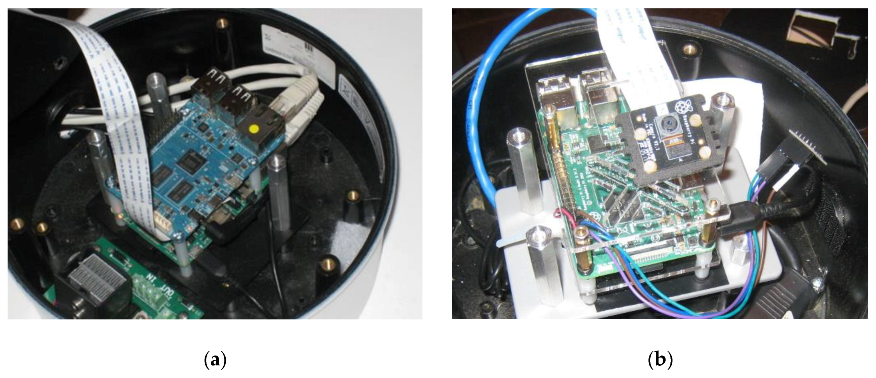
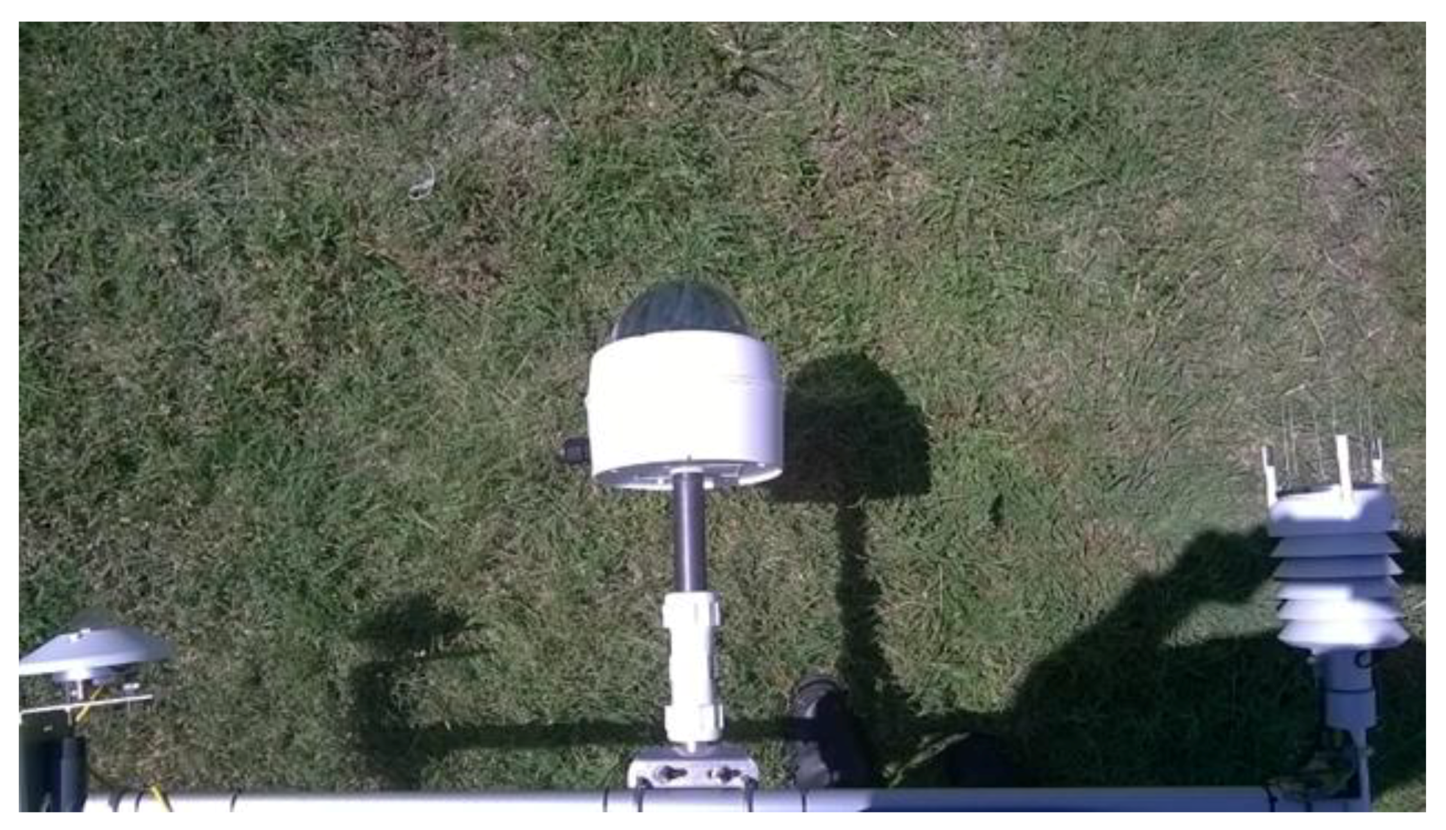
2.1. SkyImager Hardware

Figure 10a displays the original SkyImager hardware. At NREL it was found necessary to add an extra SBC for increased computational power–the Odroid C1 by Hardkernel. Heat dissipation is an issue with SBC in Texas summers. One C1 was destroyed by heat and as result a cooling fan was added to the design. The new C2 Odroid has a heat sink to eliminate the overheating issue. Acquiring and fusing the 3-exposure images could be done with just the Raspberry Pi 2. The Pi 3 model is 50% faster than its predecessor; careful optimization of the workflow will allow acquisition, processing, and forecasting with just a Pi 3. This would reduce cost and greatly simplify network connections. Figure 10b shows this configuration with a single Pi 3, plastic case, cooling fan, camera, and WeatherBoard. Images could be pushed to the cloud for processing, however, the necessary bandwidth would be substantial. The sky imagers in La Graciosa are built upon a Raspberri Pi 3 model B with no ancillary boards, and a super wide fish-eye lens (field of view over 180°). An inexpensive mini PV module was added to record irradiance at the camera locations there.

Figure 11 shows the equipment deployed on the MET tower at Ft. Sam: a Kipp&Zonen CMP11 pyranometer, the UTSA SkyImager, and a Vaisala WXT520 weather transmitter. Each of the commercial devices costs several thousand dollars; this cost prompted us to search for low-cost substitutes.

Several inexpensive alternatives to a commercial pyranometer exist [49]. Devices can be added to the GPIO pins on the Raspberry Pi. The Hardkernel Weather-Board 2 shown in Figure 12a can take not only temperature, humidity, and pressure readings (bme280 Application-Specific Integrated Circuit ASIC), but also measures light in the Visible, Infra-Red, and Ultra-Violet bands (si1132 ASIC). There is a Python interface for data retrieval. After calibration and conversion of Lux to W/m², this provides irradiance measurements and limited weather data in real time. Another ancillary device that will be useful during initial deployment of the SkyImager is a GPS locator. At $20, it looks like a small mouse for a desktop computer and plugs into a USB port. The Linux programs gpsmon and cgps can be installed on Raspbian and used to take readings of the exact position using the latest GPS satellite data. These are just two of many environmental sensors that can be connected to the Raspberry Pi. Figure 12b shows the new PiNoIR camera, which captures infrared light as well as visible. This would allow for increased contrast between low-level cumulus and high-level cirrus clouds composed of ice crystals. The SkyImager can be used for additional tasks such as air quality monitoring. Figure 12c shows the $25 MQ-131 ozone detection sensor, for example.

2.2. Image Processing Pipeline

Several additional external inputs were required for our forecasting algorithms: distortion parameters for the fish eye lens, zenith angle, True North, and most importantly the cloud base height (CBH). These inputs are used in the image processing pipeline (Figure 13) to output real-time GHI forecasts for the MGMS. A summary of the pipeline is included here, for details see [8]. (1) Distortion Removal (due to fish eye lens), (2) Cropping and Masking, (3) Calculation of “Red-to-Blue Ratio” (RBR), (4) Apply Median Filter to remove impulsive noise, (5) Thresholding to determine cloud presence, (6) Compute Cloud Cover percentage (clear/moderately-cloudy/overcast), (7) Project Clouds to height of CBH, (8) Use Optical Flow to move clouds forward in time, (9) Ray-Tracing to locate cloud shadows, and finally (10) Calculate GHI using shadow locations. Although physically correct, Step (9) Ray-Tracing is an inverse problem mathematically, hence “ill-posed”. Small errors in locating shadows can produce significant errors in the forecast irradiance. To address this issue, we investigated using artificial intelligence and neural works to predict GHI values directly from forecast cloud locations.

At NREL another raw image was acquired every 15-seconds. The pipeline described above must be fine-tuned if the processing SBC is to achieve the necessary throughput. An SBC is much more limited than a desktop server as regards CPU speed and available memory/storage, which is provided by a 32 Gb micro-SD card. The usual tradeoffs between keeping a large array in memory versus writing it to disk, are still present even though there is no disk. Efficient programming constructs are required if the goal of low cost is to be achieved. The EMS may run on a military grade RuggedCom server but the SkyImager software is constrained run on an ARM architecture. Steps in the pipeline that have little effect on the overall forecast accuracy can be eliminated. Profiling/timing runs on the optical flow algorithms will show bottlenecks that can be addressed. This is important whether a ray-tracing approach or a machine learning strategy is employed.

The goal in intra-hour solar forecasting is real time PV power predictions. Those forecasts result from a two-step process: predicting cumulus cloud locations 15-min in the future and using projected cloud locations to forecast irradiance. Each step introduces errors. Work is ongoing for Step 1 - Optical Flow: compute error metrics of the 15-min ahead image versus the actual image. Step 2 - Machine Learning takes the predicted image and computes GHI. This approach separates optical flow [50] from machine learning (ML) and allows GHI to be predicted directly from the image itself. The SkyImager can be used as a pyranometer for measuring/observing irradiance.

The training datasets for the neural networks are region-specific, if not site-specific, and require many all-sky images taken on moderately cloudy days. The weights determined for Golden, CO, will have to be fined tuned for deployment in the San Antonio area for example. Training is computationally expensive, whereas the inference or prediction is very fast and can be handled by the Pi. Research on massive deep learning networks requires Graphical Processing Units (GPU) for training and software such as Theano, Keras, or Tensorflow.

2.3. Machine Learning for Irradiance Forecasting

Machine Learning (ML) is now ubiquitous in all areas of engineering and data science. It has been used in many different ways to help solve the solar power forecasting problem, as described in [51,52]. Another area where ML is widely used is forecasting building load [53,54] which includes methods that are physics-based, statistics-based (Gaussian Process, Linear Regression), and use machine learning (Artificial Neural Network, Support Vector Machine, Deep Learning). Classic references for Deep Learning include [55,56,57] and for Convolutional Neural Networks, [58].

AI software for data mining has evolved dramatically over the last few years. In data analytics Python is the premier programming language [59] and this fully validated our decision to use it for the SkyImager project. Rapidminer (Version 8.1.001) [60] is a machine learning platform with a point and click interface. As shown in Figure 14, a data flow pipeline is established that permits the user to input a data set, select attributes to analyze, determine target and predictor variable roles, partition the data into training, validation, and sometimes testing subsets, create a logical fork to apply different subprocess models such as Random Forests or Deep Learning, run the model(s), and assess error metrics and overall performance. It is a proprietary package, but a version with somewhat reduced functionality is available for educational use. For some models Rapidminer utilizes the H2O machine learning modules (Version 3.8.2.6) [61,62]. Specifically, our Deep Learning (DL) model is found in H2O as the Python function H2ODeepLearningEstimator(). An open source Python package Scikit-Learn (Version 0.19.0) [63] allows a user to prototype and compare a variety of classification, clustering, and regression models. Neural networks and deep learning has seen the evolution of specialized software such as Keras, Theano, and Google’s Tensorflow, which recently became open source. The computational demands of training networks on big data are extreme, and this has resulted in a hardware evolution from central processing units (CPU) to graphical processing units (GPU) to special purpose tensor processing units (TPU).

Before predicting irradiance for cloudy days, consider the much simpler problem of forecasting on a clear day. The Haurwitz analytic model performs well on days with no clouds. Using physics, one can derive a closed-form functional relationship [64]: GHI_clr = 1098 [cosθ_z exp(−0.057/cosθ_z)], where θ_z is the solar zenith angle. Can neural networks learn this relationship, given a large enough dataset on which to train? The actual forecasting problem on a cloudy day is of course much harder. Information in each all-sky image is used to locate and track low-level cumulus clouds as they move between the sun and PV-arrays. It is the difference between using ML to recognize machine-written (or even hand-written) digits versus recognizing and identifying faces in a crowd of people moving down the street. Work is ongoing to identify the best features to extract from the images, to efficiently solve the intra-hour solar forecasting problem and to predict very short-term ramp events.

A critical component of any machine learning strategy is deciding which features or input variables are most strongly correlated with the labels or output variables. A second aspect involves finding a representation of the data that is compressed or sparse in some basis. This dimensionality reduction [65] can be achieved through principal component analysis (PCA) or by the simple process of discarding unimportant features in the inputs. In our studies, the label or target variables were scalars: GHI values measured atop the ESIF Building at NREL. Other choices are possible such as the value GHI_clr − GHI_mea, the deviation from the clear sky value.

Each input or example is a 3-channel RGB image from the Pi camera. In the current configuration, 3 images taken 5 seconds apart at low, medium, and high exposure times are fused using the Mertens algorithm into one raw image. As mentioned, this approach reduces over-exposure and washout in the circumsolar region. The 1024 × 768 JPEG forms the basic input measurement for both the optical flow and machine learning algorithms. Low level cumulus clouds between the sun and the PV arrays have the greatest effect on the DNI, hence on GHI. For that reason, and to satisfy the need for dimensionality reduction, the first preprocessing step is to locate the area in the image that surrounds the sun and extract a 128 × 128 subimage.

Several approaches to locating the sun in the image are possible. Calculating the zenith angle from the SOLPOS program, finding true North, and then mapping physical to pixel coordinates would require extensive calibration. It was decided to use a simple robust image processing approach that finds the maximum intensity in the image. On a clear day, this always locates the sun, but occasionally when the sun is totally obscured by broken clouds, the brightest point in the picture is actually sunlight reflected off of a nearby cloud. This can be observed in a time lapse video clip in which for a few frames the sun is not at the center of the sub-image. While the cause of some transient errors, it never lasts long and does not happen when the sun is totally obscured by a uniform cloud deck without breaks. Figure 15 shows the low exposure image used to locate and center the sun and the resulting raw fused image that will ultimately become the input to the neural networks. Lastly the subimage will be resized to a point (8 × 8) where the neural networks will train in a reasonable amount of time. In supervised learning, the neural networks require labeled training examples: ordered pairs (x, y) where x is the input vector, in this case the extracted subimage img, and y is the measured irradiance in units of Watts/m² at the time the picture was taken. Since new images are fused every 15 seconds, GHI values were treated as constant on a 60 second interval for the purposes of assigning labels for the neural network images.

Many different metrics are used in data analysis and ML for evaluating model performance.

Table 1. Regression Metrics: A actual, F forecast, µ mean.

Metric	Definition
Mean Squared Error	$\mathrm{MSE}=\left(1/n\right){\displaystyle {\displaystyle \sum }_t}{\left(A_t-F_t\right)}^2$
Normalized RMS Error	$nRMSE =\sqrt{MSE}/\rho ,\rho =\left(A_{max}-A_{min}\right)$
Explained Variance	$R^2=1-{\displaystyle {\displaystyle \sum }_t}{\left(A_t-F_t\right)}^2/{\displaystyle {\displaystyle \sum }_t}{\left(A_t-\mathsf{\mu }\right)}^2$
Mean Absolute Error	$MAE=\left(1/n\right){\displaystyle {\displaystyle \sum }_t}\left|A_t-F_t\right|$
Mean Absolute Percent Error	$\mathrm{MAPE}=\frac{100\%}{n}{\displaystyle {\displaystyle \sum }_t}\left|\left(A_t-F_t\right)/A_t\right|$

lists common ones for solar forecasting. A_t is the actual value, F_t the forecast value, and µ the mean; the summation over t can be over all observations in the ML context or over the values of a time series. The metrics provide a posteriori error bounds upon which utilities can make economic decisions. MAPE is relative L₁ error, normalized for number of observations and converted to percent. When the denominator of a fraction is close to zero, µ is used instead of A_t, a common practice when predicting spot electricity prices. Some metrics such as L₁ are more robust–less sensitive to outliers–than the classical RMS error norms.

2.4. Stereographic Method for CBH Estimation

Obtaining CBH from paired sky images has been done by several authors in the past. For instance, the method proposed in [46] generated blocks of clouds which are computed to make a 3D reconstruction of the clouds. Then, the authors were able to obtain the height of the clouds by using geometric computation. On the other hand, the method in [66] used the cross correlation of non-projected saturation images to find all possible combinations that yield feasible heights, selecting the most correlated one (or the one with the minimum error).

In the GRACIOSA project, a pure geometric method based on the relative position of the sky-imagers and the clouds was implemented. First, the algorithm looks for the same cloud feature in the images coming from the two sky-imagers. This task can be extremely difficult due to the chaotic nature of clouds and slight changes in image properties such as luminosity. But fortunately, a Scale-Invariant Feature Transform (SIFT) algorithm [67], can handle this situation. This algorithm performs excellently, identifying features in a constantly changing shape (as clouds), since it considers possible changes in scale and orientation. SIFT is applied to pairs of simultaneous images from both cameras (Figure 16). Once the features from both images have been paired up, the best matches are selected to continue the calculations. Valid features are then transposed from the image (pixels) to real space (azimuth and zenith). With real space coordinates defined and the projection matrix of the lenses known, geometric computation is used to obtain the length of the vectors containing each feature and the geographical position of each camera in real space, from which the height of the evaluated feature can be derived.

3. Results

Almost a terabyte of image data was collected at NREL from 15 October 2015 through 16 April 2016. The measured DNI values were recorded using NREL’s CHP1-L pyranometer with units of Watts/m². Days were grouped into three categories: (1) Clear Sky; consisting of predominantly clear days with little or no cloud cover; (2) Overcast; large masses of clouds that obscure the sun for most of the day; and finally (3) Moderately Cloudy; characterized by large variation in irradiance values and multiple ramp events. For Clear Sky and Overcast conditions there is no forecasting to do –persistence can’t be beat. Other cloud cover classifications are possible. One could use unsupervised ML clustering algorithms on the raw irradiance data to find other breakdowns. Standard METAR cloud classification separates clouds into low, middle, and high level. All clouds affect measured irradiance [68]. We focus on cumulus clouds because they have the greatest effect on ramp events.

Prediction of intra-hour GHI can be partitioned into several distinct sub-tasks. (1) Acquiring a time series of all-sky images. Every 15 s a new raw image is fused [69] from three different exposure times to allow for High Dynamic Range (HDR) [70]. (2) Using the recent past images and optical flow to extrapolate cloud locations 15 min into the future. It is possible to enhance the algorithm, but it must not hamper production of real time forecasts. (3) Using the predicted image and the weights from training the neural network, a predicted GHI value is output to the microgrid management system.

In the original configuration, our software used optical flow to track movement of cumulus clouds and then ray tracing to predict cloud shadow locations. A better methodology would utilize artificial intelligence (AI) to classify the reduction in GHI that will result when cumulus clouds are predicted in the circumsolar region. It is expensive to train neural networks, but this is done offline for a given location. Once optimal weights are determined, the calculation of a single GHI value is very fast–amounting to an inner product. If the optical flow calculation requires too much time, a second single board computer can be added to the hardware as was employed at NREL.

Details of our research on machine learning to predict solar irradiance are described in the paper [9]. Our intent here is to provide the reader with a concise summary of that research. A critical outcome was verification that the SkyImager with the Pi camera can measure GHI in real time. Lacking the accuracy of an expensive pyranometer, this approach would use the image sequence acquired to solve the forecasting problem, in order to simultaneously estimate GHI. This data could be incorporated with readings from the WeatherBoard to provide additional inputs to the MGMS using MQTT or DDS protocols. Variables that are considered deterministic should be treated as stochastic random variables. Convolutional neural networks [58] which preserve spatial information offer the best performance for image datasets. Expensive offline training of the networks is normally done one time but it is possible to do continuous learning where the networks use feedback in the form of newly acquired data to refine the learned weights.

In the field of machine learning, there are standard ways of visualizing both the input dataset consisting of vectors in a high dimensional space, as well as targets and predicted outputs. The UTSA SkyImager collected all images in this study on the ESIF building rooftop at NREL as part of the INTEGRATE project. During 147 days from October, 2015 until May, 2016 there were 14 days of no data collected (technical reasons) and 27 days of partial data collection. The remaining 106 days of no missing data formed the inputs for training and testing the neural networks. This yielded 156,495 observations (examples or rows) for input to the neural networks. We used the standard split (70% − 30%) of the data into training and testing subsets: 109,547 examples for training and 46,948 for testing.

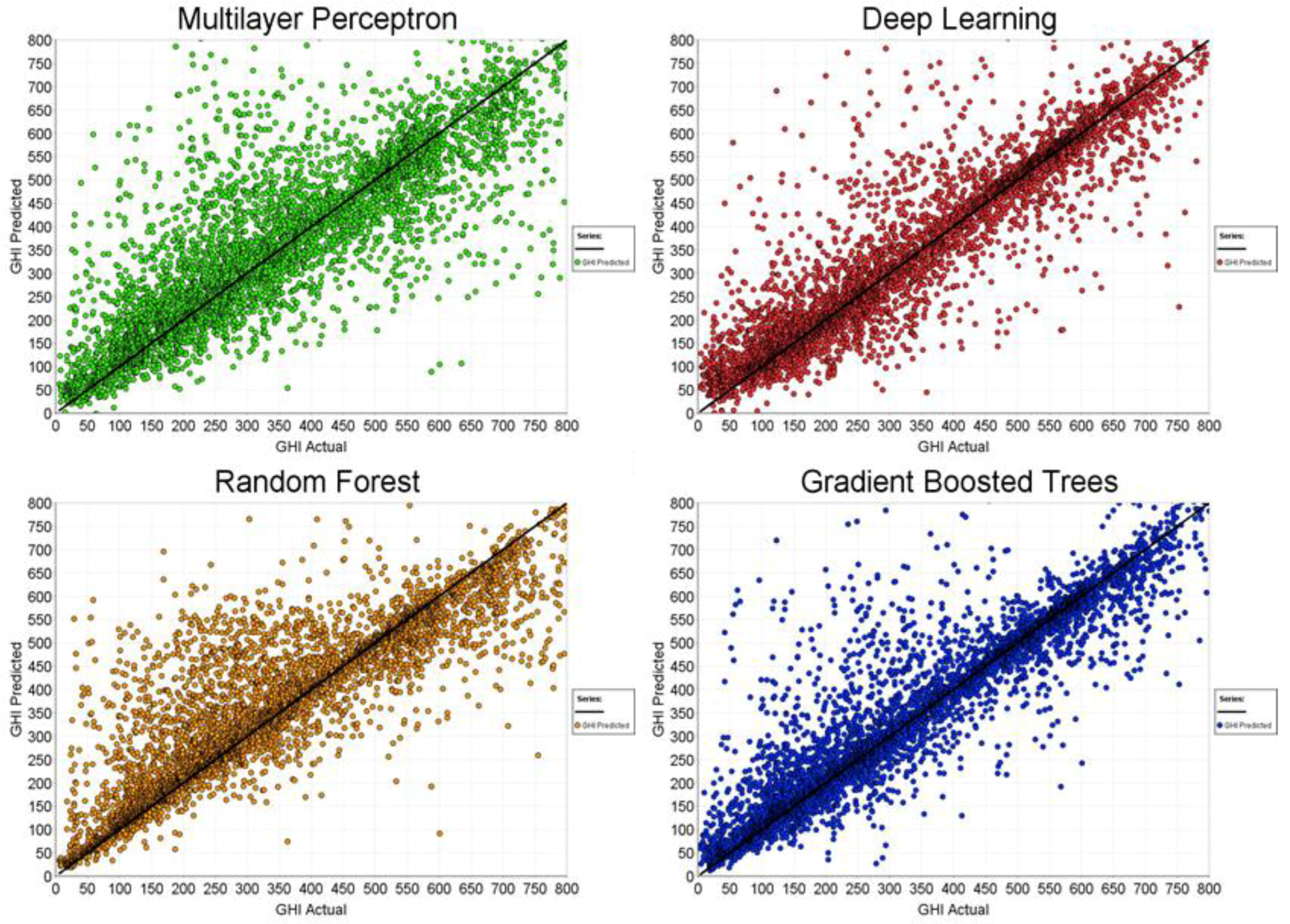
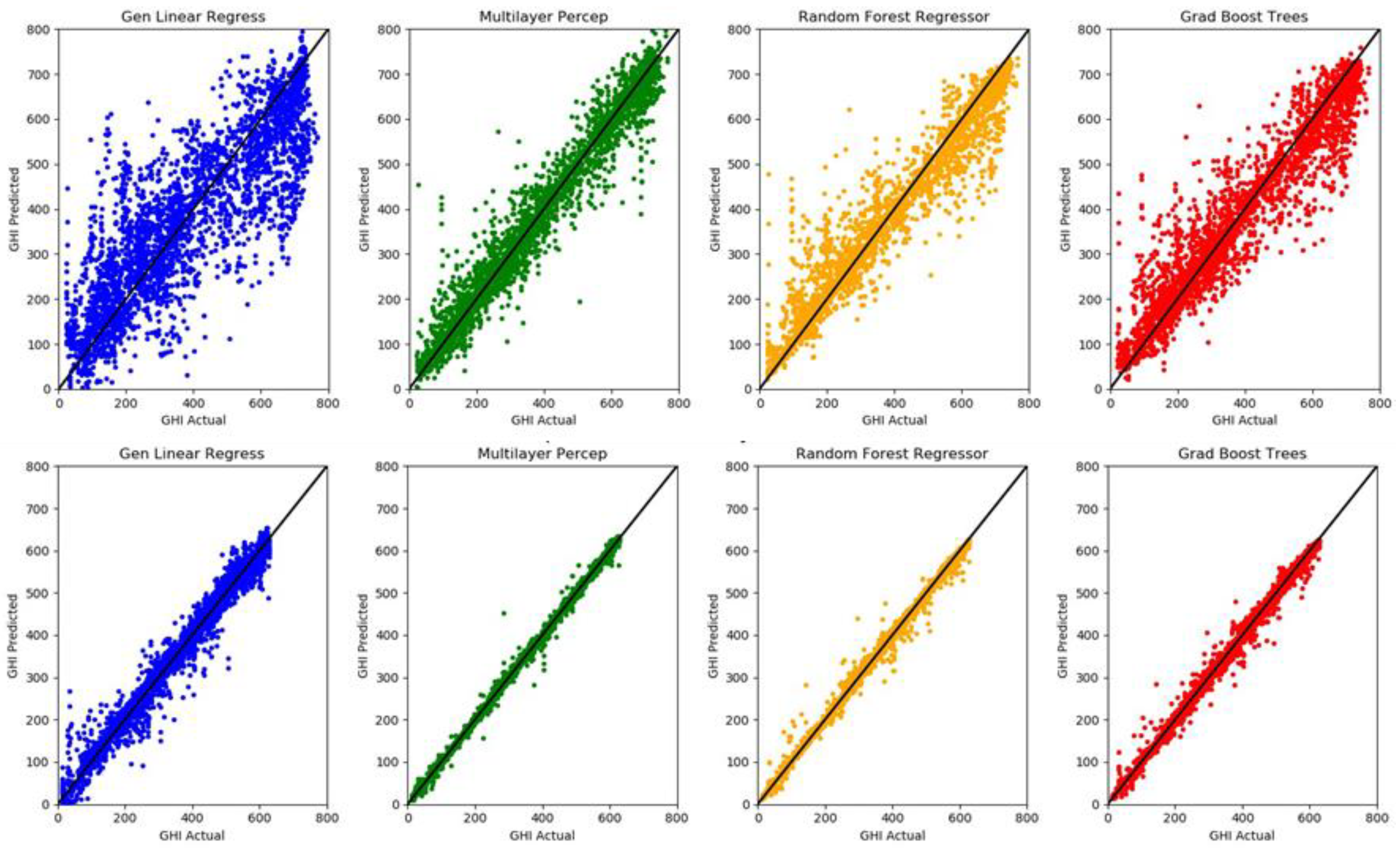
3.1. Comparing 4 Different ML Models

Each input example is uniquely associated with one of the SkyImager pictures taken every 15 s. The normalized pixel values for the Red-Green-Blue (RGB) channels of an 8 × 8 resized subimage centered about the sun are flattened into one row vector. Note that other color spaces such as HSV or HSL could also be used. Resizing provided dimensionality reduction and reduced runtimes, but with substantial computer resources the 128 × 128 sub-images could be used for training. Average values of each channel were included as additional features for a total of 3 × 64 + 3 = 195 features. The first entry in each row is the measured GHI in W/m². To show how well random variables X and Y are correlated, one uses a scatter diagram. Figure 17 shows scatter diagrams of measured GHI versus predicted GHI for four ML models: Multi-Layer Perceptron (MLP), Random Forest (RF), Deep Learning (DL), and Gradient Boosted Trees (GBT). While all models perform well (tight clustering around y = x, perfect correlation), DL and GBT have fewer outliers and visually outperform the other two models.

Note that the MLP and RF models were run using the Scikit-Learn ML software package while DL and GBT were run on the Rapidminer platform. This validated our results on different ML packages—results should depend on the algorithms, not the platform on which they are implemented. Currently, Scikit-Learn does not offer a deep learning model. Using Rapidminer is very convenient on a powerful desktop PC, our ultimate goal is to use the trained weights on a Raspberry Pi 3 computer for real time forecasting. Scikit-Learn with its open source Python interface should prove valuable for that task.

MAE, MAPE, nRMSE, and R² error metrics are given in

Table 2. Evaluation of four machine learning models.

ML Model	Platform	Runtime (min)	MAE	MAPE	nRMSE	RR2
Multilayer Perceptron	Scikit-Learn	3:05	81.21	33.05%	32%	0.71
Random Forest	Scikit-Learn	14:53	66.86	28%	29%	0.76
Deep Learning	Rapidminer	43:52	50.992	27.13%	21.6%	0.871
Gradient Boosted Trees	Rapidminer	4:50	47.072	22.73%	21.1%	0.875

and run times in minutes. The explained variance (R²) in the last column is very significant. Both DL and GBT achieve values of 0.87, while MLP and RF are 0.1 less. The other error metrics closely track the R² values. In DL the extra accuracy is at the expense of much longer run times, but GBT gets the highest accuracy and is very fast: 10 min faster than RF.

A time series is another approach to visualizing the results: GHI values are plotted on the y-axis and time on the x-axis. Figure 18 compares measured and predicted GHI for one day, 3 October 2015. Although there are differences in the two curves, they track each other well. More illuminating is a time series display for the entire group of testing days shown in Figure 19, where actual GHI is blue and forecast values are red. It is difficult to distinguish the two curves because they track each other so closely. For both figures the deep learning model was used for prediction. Observe in the center of Figure 19 a group of five consecutive clear sky days that are easy to predict, as are completely overcast days.

The two curves differ most on moderately cloudy days with air mass cumulus clouds present.

3.2. Different Deep Learning Model Results

Machine learning algorithms have many hyper-parameters that can be optimized to improve accuracies and reduce run times.

Table 3. Comparison of 4 Deep Learning Models.

Hid. Layer	Nodes per H. Layer	# Epochs	Run Time	MAE	MAPE	nRMSE	R2
2	50,50	10	1:55 min	65.807	32.73%	25.8%	0.815
2	195,195	10	7:10 min	66.872	40.76%	25.6%	0.824
3	195,195,195	500	43:52 min	50.992	27.13%	21.6%	0.871
5	195,195,97,195,195	100	67:42 min	48.519	26.09%	21.6%	0.871

shows how changing the number of hidden layers for the DL model, nodes in the layers, and number of epochs (complete passes through the training dataset) affects results. Model 1 has 2 hidden layers each with 50 nodes; it requires ten epochs to train with a run time of ~2 min and R² = 0.815. Model 2 also has two hidden layers (195,195) and 10 epochs, but runs 3 times longer and only improves R² to 0.824. To achieve R² = 0.871 Model 3 (195,195,195) needs 500 epochs and ~45 min. A point of diminishing returns is reached: Model 4 (195,195,97, 195,195) takes more than an hour to run on a desktop PC. Further improvements in accuracy would require larger input images or tuning DL parameters.

3.3. Cloudy Versus Clear Sky Days

From each 1024 × 768 fused raw image, the algorithm extracts a 128 × 128 pixel subimage centered on the sun. Using the transform.resize function from Skimage, this is resized to 8 × 8 pixels to achieve dimensionality reduction. This idea is critical to successful machine learning: each example in the dataset is a vector in a high-dimensional space and there are many examples. Principal Component Analysis and Linear Discriminant Analysis are other techniques for reduction, but our approach is simple and has proved to be effective.

In the following case study ten days of SkyImager data acquired at NREL were used to synthesize two datasets. Five moderately cloudy days comprised the first dataset, October 16, 17, 18, 19, 20 in 2015. Five clear sky days of data from November 10, 11, 12, 13, 14 of 2015 made up the second dataset. The neural networks were fed 32 × 32 pixel resized images and 4 ML models from Scikit-Learn were compared: Generalized Linear Regression Model (GLM), Multi-Layer Perceptron (MLP), Random Forest Regressor (RFR), and Gradient Boosted Trees (GBT).

Table 4. Results for two datasets of 32 × 32 resized sub-images.

	5 Moderately Cloudy Days				5 Clear Sky Days
Model Name	GLM	MLP	RFR	GBT	GLM	MLP	RFR	GBT
MAPE	39.75	13.53	15.79	20.93	12.0	2.44	2.66	3.79
Explained Variance R2	0.70	0.95	0.93	0.90	0.97	1.00	1.00	0.99
Mean Absolute Error	86.43	30.66	33.30	44.68	20.43	5.30	5.84	8.57
Elapsed Time (Sec)	0.1	513.1	69.9	12.4	0.1	512.8	60.5	12.0

and Figure 20 show the results. GLM and GBT have much shorter runtimes in both cases, while MLP and RFR achieve higher R² values. Maximum accuracies are achieved with MLP but at a cost of increased runtimes. Extreme accuracy in R² values for clear sky days (0.97, 1.0, 1.0, 0.99) indicates the networks are learning the analytic form of the Haurwitz clear-sky GHI model well.

Using still finer sampling for the resized sub-images should yield better results at the cost of larger data files and runtimes. At some point however, statistics suggests diminishing returns. In addition to detailed descriptions of ML models and software our article [9] presents another case study. It uses only one moderately cloudy day (17 October 2015) of observations and runs the four ML models with 8 × 8, 32 × 32, and 64 × 64-pixel sub-images. The size of the CSV input data file increases quickly: 3 Megabytes, 111 Mb, and 442 Mb, as do runtimes 139 s, 444 s, and 1309 s. Accuracies improve, but not beyond a certain point.

3.4. JBSA Microgrid Data

The JBSA microgrid was built as a testbed for the CPS Energy Grid Modernization Laboratory. Management and control of a microgrid must address many factors including cybersecurity, data acquisition, data management, real-time computation, storage, bandwidth, interoperability, and usability requirements. In addition to the data acquired by the UTSA equipment–SkyImager, WXT520 Vaisala weather station, and pyranometer; this includes 36-hour ahead hourly weather forecasts scraped from the web, the day-ahead Load/PV forecasts, battery State-Of-Charge (SOC) readings, actual load for the base library building, and control data from the Siemens MGMS. The goal is to use all available data in order to refine site-specific solar irradiance forecasts for improved operation and control of the microgrid. Non-UTSA data from the JBSA microgrid was acquired from Itron MV-90 xi meters. This is a system used for the collection and management of interval data consisting of time stamped readings taken every x minutes where x can be 5, 15, 30, or 60. A large electric utility may acquire a billion interval readings in a single year and use them in a variety of ways including billing (demand response, real time pricing, curtailable rates), open market operations, and load/market research.

Analyses of the JBSA MV90 data, all of which were taken at 15 min intervals, demonstrated that much finer temporal resolution would be required to capture details of ramp events and provide accurate irradiance forecasts to the MGMS. While 1 min resolution was provided by the UTSA equipment such as the pyranometer and Vaisala weather station, the cost of this equipment precluded widespread deployment in a distributed environment. Similar equipment at the UTSA solar testbed provided a wealth of 1 min data, but we envisioned a network of hundreds of low cost SkyImagers spread across the city of San Antonio, and for this scenario low cost was an essential requirement. As previously discussed, there are a plethora of low-cost sensors that can be connected to the GPIO pins on a SBC, including the WeatherBoard2 (WB2), air quality and ozone sensors, and even devices to measure dust. Costing tens of dollars they provide a cost-effective way of environmental sensing that can easily be incorporated with the SkyImager. Figure 21 shows observations of irradiance, temperature, humidity, and pressure taken every minute on 26 November 2018 with the WB2 sensor mounted on a SkyImager.

The mini photovoltaic module used at ULL is an off-the-shelf PV module, made of c-Si, with open circuit voltage of 6V and a short circuit current of 200 mA, with a maximum DC output of 1.1 W. The module was connected to a resistive load to dissipate the heat, and the data was registered by a INA219 DC Current Sensor able to measure very small currents, attached to the Raspberry Pi 3 model B.

3.5. One Second Minimodule Data from La Graciosa

The Universidad de La Laguna in the Canary Islands provided 1 sec data from the minimodule at the La Graciosa microgrid operated by ENDESA. How does the spectral content of the voltage signal change when moving from 1 s, 5 s, 15 s, to 60 s sampling? Figure 22 shows the effect of sub-sampling on the time-series. Some of the noise present in the data might be due to voltage fluctuations or seagulls (the location was the Fisherman’s Guild building). Certainly the area of the minimodule is very small, so it behaves as a point measurement where small occulding objects can drastically the affect irradiance measurements. Still, the analysis strongly suggests that to resolve the frequency and voltage swings that occur during a sudden ramp event, PMU measurements may be a necessity.

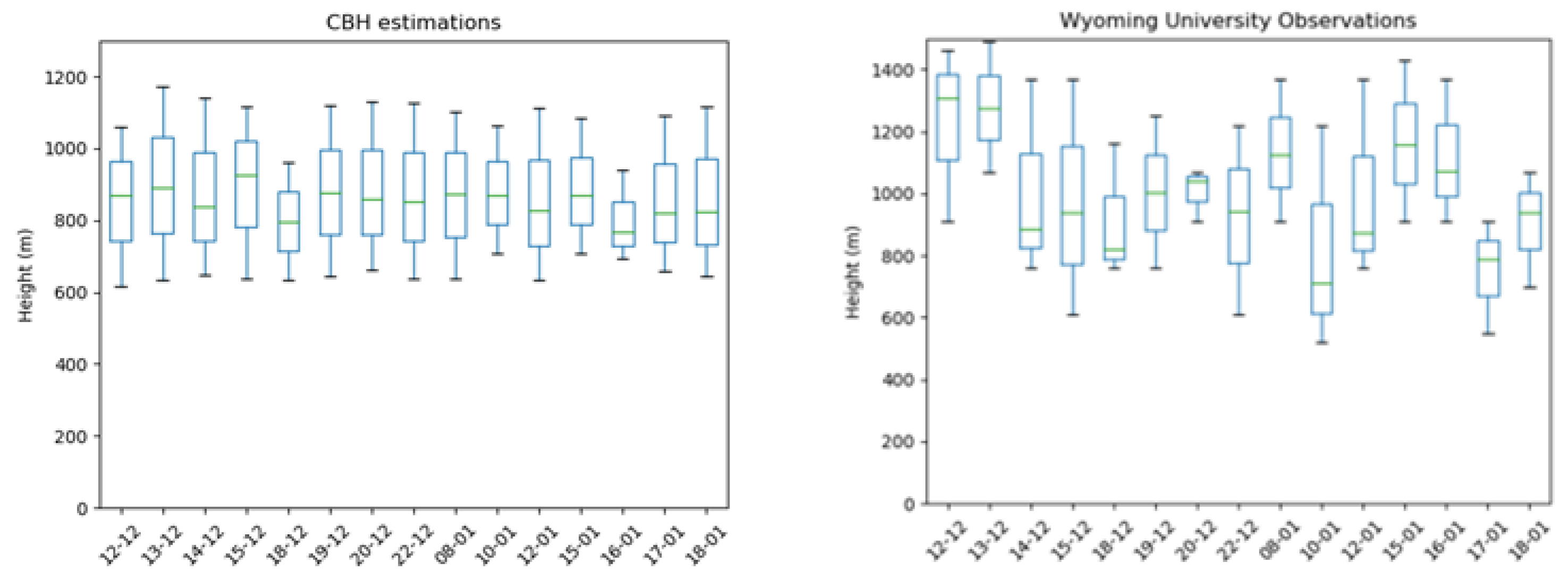
3.6. CBH Estimations

The results of the CBH estimations are presented in Figure 23. The left boxplot shows the statistical distribution of the heights obtained with the stereographic method, while the right boxplot shows the statistical distribution of a weather station located in Arrecife, Lanzarote, which belongs to the network of the University of Wyoming.

There are several reasons for the apparent mismatch in the data. First, the weather station is located 30 km south of the position of the cameras, which undoubtedly has a significant effect taking into account how the atmospheric conditions develop in the region (with the thermal inversion steadily rising its level from the Sahara Desert). Second, the data of the weather station is obtained using a punctual measurement such as LIDAR, while the CBH estimations of the cameras cover a larger area of the sky (mainly the central part of the fish-eye image, since the distortion on the borders makes it almost impossible to compute the height). Finally, the temporal resolution of the weather station data is up to 1 hour, while the estimation of the CBH by the stereographic approach is done every minute. Likely the most important conclusion here is that the estimations made by the systems are coherent with the previous knowledge of the atmospheric conditions, with a stable thermal inversion ranging from 600 to 2000 m depending on the season of the year, which prevents clouds to rise over a certain height.

4. Discussion

Our future research efforts will be directed in several areas. Optical flow is a critical area for the success of intra-hour solar forecasting. IoT and cyber-security also form a critical component. Solving the AC Optimal Power Flow equations with GHI forecasts from the SkyImager will be important for solving the energy storage and microgrid control problems. Using the Raspberry Pi additionally as a multiple-sensor platform will be investigated. Environmental studies of the effects of dust and bird feces on the solar panels may well utilize SkyImager technology.

It was on the INTEGRATE project that a synergism developed between researchers and engineers at the national lab, universities, utilities, and private industry that continued after the project ended. Management styles are quite different in academia and private industry with national labs somewhere in between. Software version control was critical, as was careful documentation of all work. Both for the utility where engineers would use the hardware/software and for the university where graduate students and faculty would move on to other projects this was very important. Our decision to use Python was an excellent one. Increasingly, both documentation, tutorials, and example programs are being delivered in the form of IPython notebooks (.IPNB files) as, for example, Google’s Tensorflow. Even a package such as Open Computer Vision [71,72] that is written in C++ for efficiency has Python bindings that allow easy access to routines for image fusion and optical flow.

4.1. Lessons Learned at the 3 Deployment Locations

4.1.1. SkyImager at NREL

The NREL microgrid was located at a specialized research facility, but every attempt was made to simulate conditions at a utility. The communications network was well established; there was abundant state-of-the-art ancillary equipment such as pyranometers and an on-site weather station, and the process of deployment went relatively smoothly. Still there were important lessons to be learned. The SkyImager was initially configured with a single Raspberry Pi 2, which proved insufficient for both acquiring images and processing them through the pipeline to produce irradiance forecasts. This problem was solved by adding an Odroid C1, but this made the design more complex and required bridging between the two SBC using a USB-internet connection. The plethora of operating systems for both the SBC and EMS servers provided still another challenge. There are differences in the way open source packages such as OpenCV and Mosquitto install and operate on Raspbian, Ubuntu 14, and Ubuntu 16. In some cases, there are compiled binaries available and in others software must be compiled from source files. From a solar forecasting perspective, NREL was where the best, most complete data was acquired: over six months of daily images and ground truth pyranometer observations. It took researchers over a year to analyze the data and the process is ongoing.

4.1.2. SkyImager at San Antonio, TX, USA

Two critical applications of islanded microgrids are remote installations in developing countries and power systems for the military that must be entirely stand alone. While this made a military base the perfect site for testing a microgrid EMS, it also meant that obtaining base access for UTSA researchers was an issue. For safety purposes, it requires at least two people to lower the 10 m MET tower. Beyond the initial installation, access to the tower is required every month to inspect the instruments and clean the surface of the plastic dome that covers the camera enclosure. The cost of the pyranometer and weather station exceeded that of the SkyImager by a factor of 20 and prompted adding low-cost sensors to the SBC for measuring temperature, humidity, and light.

Occasional loss of power to the SBC as the battery went through its initial testing phase was a minor issue which required tinkering so that the forecasting software was immediately brought back on line during a reboot. Initially the Mosquitto MQTT broker was chosen for the UTSA software, but because of compatibility issues with the MyRio software, HiveMQ proved to be a better choice. Direct internet access to our SBC from outside the corporate network was available only through a WebEx session that required close coordination between the utility and university personnel. Lesson learned: when initially transitioning hardware/software from a research environment to a production one, it is imperative to have physical/cyber access to the equipment and network. Several Odroid’s were damaged by high temperatures in the enclosure boxes and had to be replaced. MV90 meter readings every 15 min are clearly insufficient for the intra-hour forecasting problem. We are currently working with a group in Austin to add inexpensive Phasor Measurement Units (PMU) to acquire detailed frequency and phase information in conjunction with weather, irradiance, and sky images. Cloud computing [73] and 5G networks offer unique opportunities to move most of the computations off the Raspberry Pi to the cloud.

4.1.3. SkyImager at La Graciosa, Canary Islands

Some valuable lessons learned from the Graciosa project have to do with the performance and durability of the sky-imagers in a harsh, dusty, and salty environment such as La Graciosa. The closeness of the island to the Sahara Desert makes the dust content in the atmosphere high. Quality of the images is severely affected by the deposition of dust on the enclosure, as seen in Figure 24, showing that scheduled cleanings of the enclosure are necessary to ensure the proper function of the devices. Our first estimation is that cleaning is necessary at least twice a year, but it is highly dependent on the climatologic and atmospheric conditions. Besides the deposition of dust on the enclosure, water infiltrations in the interior of the enclosure have been a frequent problem, even if the equipment was specially selected to have a high degree of protection to water and dust (IP67). Closeness to the sea, as well as the strong rains that occurred in December of 2017, appear to be the main source of this problem.

5. Conclusions

In March of 2018 the California Energy Commission mandated that beginning in 2020, all new home and apartment construction must include solar generation. When this level of distributed generation becomes part of the electric grid, ISO are faced with new challenges in terms of frequency and voltage control. Indeed, in Hawaii these issues resulted in a temporary hold on rebates for new residential solar installations.

In a macrogrid extending over hundreds of square kilometers, integrating a mix of generation conventional power plants, solar, and wind, and functioning as part of a larger interconnect such as ERCOT, there is an inherent inertia that works on the side of the utility. In microgrids, however, this inertia is lacking, and the control problem becomes much more difficult to solve when in islanded mode [4,7]. There are also different temporal scales involved. Optimal day-ahead scheduling and control of a microgrid is a distinct problem from hour-ahead control to ensure frequency and voltage do not vary outside prescribed limits. Using equipment such as the OP4500 RT-LAB/RCP/HIL real-time power grid digital simulator by Opal RT, we hope to use Hardware-in-the-Loop equipment to analyze the microgrid at JBSA. PMU measurements also need to be incorporated.

All-sky imaging technology will be a critical component in the overall solution strategy to predict solar irradiance 15 min ahead, and to take corrective measures during ramp events. It must, however, be fully integrated with NWP and satellite-based approaches for day-ahead load forecasting and optimal control of a microgrid. Optimal use of this technology will encompass a diverse group of specializations, including IoT and edge-computing, cyber-security, machine learning, and image processing.

For example, the characteristics and statistics of the all-sky imager must be included in the stochastic optimization programming for risk neutral and risk adverse operational control of a microgrid [6]. An holistic R&D approach is required. While a Raspberry Pi is the essence of plug-N-play and it is relatively straightforward to build a SkyImager, integration into the IoT and field deployment will remain an active area of research. Imagers will range the gamut in cost, accuracy, and interoperability. MGMS will integrate forecasts from imagers, NWP, and satellites, as well as hundreds of other meters and devices to solve the microgrid control problem. While physics-based methodology will continue to be important, machine learning and IoT technology will play an increasingly critical role. Development of standards such as OpenFMB for interoperability of thousands of devices will also be a necessary component.

6. Patents

A provisional US patent application “distributed solar energy prediction imaging” has resulted from the work reported in this manuscript.

References

1. Guerrero-Lemus, R.; Shephard, L. Low Carbon Energy in Africa and Latin America: Renewable Technologies, Natural Gas and Nuclear Energy (Lecture Notes in Energy), 1st ed.; Springer: Berlin, Germany, 2017. [Google Scholar]
2. Available online: https://uc-ciee.org/downloads/appendixA.pdf (accessed on 16 February 2019).
3. Janssen, T.; Krishnaswami, H. Voltage and Current Control of a Multi-port NPC Inverter Configuration for a Grid-Connected Photovoltaic System. In Proceedings of the IEEE 17th Workshop on Control and Modeling for Power Electronics, Trondheim, Norway, 27–30 June 2016. [Google Scholar]
4. Olivares, D.; Lara, J.; Canizares, C.; Kazerani, M. Stochastic-Predictive Energy Management System for Isolated Microgrids. IEEE Trans. Smart Grid 2015, 6, 2681–2693. [Google Scholar] [CrossRef]
5. Canizares, C.; Palma-Behnke, R.; Olivares, D.; Mehrizi-Sani, A.; Etermadi, A.; Iravani, R.; Kazerani, M.; Hajimiragha, A.; Gomis-Bellmunt, O.; Saeedifard, M.; et al. Trends in Microgrid Control. IEEE Trans. Smart Grid 2014, 5, 1905–1919. [Google Scholar]
6. Farzan, F.; Jafari, M.; Masiello, R.; Lu, Y. Toward Optimal Day-Ahead Scheduling and Operational Control of Microgrids Under Uncertainty. IEEE Trans. Smart Grid 2015, 6, 499–507. [Google Scholar] [CrossRef]
7. Michaelson, D.; Mahmood, H.; Jiang, J. A Predictive Energy Management System Using Pre-Emptive Load Shedding for Islanded Photovoltaic Microgrids. IEEE Trans. Ind. Electron. 2017, 64, 5440–5448. [Google Scholar] [CrossRef]
8. Jr, W.R.; Krishnaswami, H.; Vega, R.; Cervantes, M. A low cost, edge computing, all-sky imager for cloud tracking and intra-hour irradiance forecasting. Sustainability 2017, 12, 482. [Google Scholar]
9. Moncada, A.; Richardson, W., Jr.; Vega-Avila, R. Deep Learning to Forecast Solar Irradiance Using a Six-Month UTSA SkyImager Dataset. Energies 2018, 11, 1988. [Google Scholar] [CrossRef]
10. Nummikoski, J.; Manjili, Y.S.; Vega, R.; Krishnaswami, H. Adaptive Rule Generation for Solar Forecasting: Interfacing with A Knowledge-Base Library. In Proceedings of the IEEE 39th Photovoltaic Specialists Conference (PVSC), Tampa, FL, USA, 16–21 June 2013. [Google Scholar]
11. Cervantes, M.; Krishnaswami, H.; Richardson, W.; Vega, R. Utilization of Low Cost, Sky-Imaging Technology for Irradiance Forecasting of Distributed Solar Generation. In Proceedings of the IEEE GreenTech Conference, Kansas City, MO, USA, 6–8 April 2016. [Google Scholar] [CrossRef]
12. Cañadillas, D.; Richardson, W., Jr.; González-Díaz, B.; Shephard, L.; Guerrero-Lemus, R. First Results of a Low Cost All-Sky Imager for Cloud Tracking and Intra-Hour Irradiance Forecasting serving a PV-based Smart Grid in La Graciosa Island. In Proceedings of the IEEE PVSC-44, Washington, DC, USA, 25 June 2017. [Google Scholar]
13. Richardson, W.; Krishnaswami, H.; Shephard, L.; Vega, R. Machine Learning versus Ray-Tracing to Forecast Irradiance for an Edge-Computing SkyImager. In Proceedings of the 19th International Conference on Intelligent System Application to Power Systems (ISAP), San Antonio, TX, USA, 17–20 September 2017. [Google Scholar]
14. Waight, J.; Grover, S.; Laval, S.; Shephard, L.; Boston, J.; Lui, R.; Mathew, J.; Bradley, D.; Lawrence, D.; Sparkman, M.; et al. NREL Integrate: RCS -4-42326: Topic Area 3 OpenFMB Reference Architecture Demonstration Final Report, Minneapolis, 2017.
15. Mathiesen, P.; Kleissl, J. Evaluation of numerical weather prediction for intra-day solar forecasting in the continental United States. Solar Energy 2011, 85, 967–977. [Google Scholar] [CrossRef]
16. Available online: https://www.ncdc.noaa.gov/data-access/model-data/model-datasets/rapid-refresh-rap (accessed on 20 December 2018).
17. Xia, S.; Mestas-Nuñez, A.M.; Xie, H.; Vega, R. An Evaluation of Satellite Estimates of Solar Surface Irradiance Using Ground Observations in San Antonio, Texas, USA. Remote Sens. 2017, 9, 1268. [Google Scholar] [CrossRef]
18. Mueller, R.; Trentmann, J.; Träger-Chatterjee, C.; Posselt, R.; Stöckli, R. The Role of the Effective Cloud Albedo for Climate Monitoring and Analysis. Remote Sens. 2011, 3, 2305–2320. [Google Scholar] [CrossRef] [Green Version]
19. Urbich, I.; Bendix, J.; Muller, R. A Novel Approach for the Short-Term Forecast of the Effective Cloud Albedo. Remote Sens. 2018, 10, 995. [Google Scholar] [CrossRef]
20. Perez, R.; Ineichen, P.; Moore, K.; Kmiecik, M.; Chain, C.; George, R.; Vignola, F. A New Operational Model for Satellite-Derived Irradiances: Description and Validation. Solar Energy 2002, 73, 307–317. [Google Scholar] [CrossRef]
21. Law, E.; Prasad, A.; Kay, M.; Taylor, R. Direct normal irradiance forecasting and its application to concentrated solar thermal output forecasting: A review. Solar Energy 2014, 108, 287–307. [Google Scholar] [CrossRef]
22. Raza, M.Q.; Nadarajah, M.; Ekanayake, C. On recent advances in PV output power forecasting. Sol. Energy 2016, 136, 125–144. [Google Scholar] [CrossRef]
23. Barbieri, F.; Rajakaruna, S.; Gosh, A. Very short-term photovoltaic power forecasting with cloud modeling: A review. Renew. Sustain. Energy 2017, 75, 242–263. [Google Scholar] [CrossRef]
24. Antonanzas, J.; Osorio, N.; Escobar, R.; Urraca, R.; Martinez-de_Pison, F.; Antonanzas-Torres, F. Review of photovoltaic power forecasting. Solar Energy 2016, 136, 78–111. [Google Scholar] [CrossRef]
25. Marquez, R.; Coimbra, C. Intra-hour DNI forecasting based on cloud tracking image analysis. Sol. Energy 2013, 91, 327–336. [Google Scholar] [CrossRef]
26. Marquez, R.; Coimbra, C. Proposed Metric for Evaluation of Solar Forecasting Models. J. Sol. Energy Eng. 2013, 135, 011016. [Google Scholar] [CrossRef]
27. Gohari, S.; Urquhart, B.; Yang, H.; Kurtz, B.; Nguyen, D.; Chow, M.; Kleissl, J. Comparison of solar power output forecasting performance of the Total Sky Imager and the University of California, San Diego Sky Imager. Energy Procedia 2014, 49, 2340–2350. [Google Scholar] [CrossRef]
28. Urquhart, B.; Kurtz, B.; Dahlin, E.; Ghonima, M.; Shields, J.; Kleissl, J. Development of a sky imaging system for short-term solar power forecasting. Atmos. Meas. Tech. Discuss. 2014, 7, 4859–4907. [Google Scholar] [CrossRef]
29. Chow, C.W.; Urquhart, B.; Lave, M.; Dominguez, A.; Kleissl, J.; Shields, J.; Washom, B. Intro-hour forecasting with a total sky imager at the UC San Diego solar energy testbed. Sol. Energy 2011, 85, 2881–2893. [Google Scholar] [CrossRef]
30. Chu, Y.; Pedro, H.; Coimbra, C. Hybrid intra-hour DNI forecasts with sky image processing enhanced by stochastic learning. Sol. Energy 2013, 98, 592–603. [Google Scholar] [CrossRef]
31. Yang, H.; Kurtz, B.; Nguyen, D.; Urquhart, B.; Chow, C.; Ghonima, M.; Kleissl, J. Solar irradiance forecasting using a ground-based sky imager developed at UC San Diego. Sol. Energy 2014, 103, 502–524. [Google Scholar] [CrossRef]
32. Bernecker, D.; Riess, C.; Angelopoulou, E.; Hornegger, J. Continuous short-term irradiance forecasts using sky images. Sol. Energy 2014, 110, 303–315. [Google Scholar] [CrossRef]
33. West, S.; Rowe, D.; Sayeef, S.; Berry, A. Short-term irradiance forecasting using skycams: Motivation and development. Sol. Energy 2014, 110, 188–207. [Google Scholar] [CrossRef]
34. Wood-Bradley, P.; Zapata, J.; Pye, J. Cloud tracking with optical flow for short-term solar forecasting. In Proceedings of the Conference of the Australian Solar Energy Society, Melbourne, Australia, 21 August 2012. [Google Scholar]
35. Wang, F.; Zhen, Z.; Mi, Z.; Sun, H.; Su, S.; Yang, G. Solar irradiance feature extraction and support vector machines based weather status pattern recognition model for short-term photovoltaic power forecasting. Energy Build. 2014, 86, 427–438. [Google Scholar] [CrossRef]
36. Zhu, T.; Wei, H.; Zhang, C.; Zhang, K.; Liu, T. A Local Threshold Algorithm for Cloud Detection on Ground-based Cloud Images. In Proceedings of the 34th Chinese Control Conference, Hangzhou, China, 28–30 July 2015. [Google Scholar]
37. Peng, Z.; Yoo, S.; Yu, D.; Huang, D. Solar Irradiance Forecast System Based on Geostationary Satellite. In Proceedings of the IEEE International Conference on Smart Grid Communications (SmartGridComm), Vancouver, BC, Canada, 21–24 October 2013. [Google Scholar]
38. Yang, D.; Kleissl, J.; Gueymard, C.; Pedro, H.; Coimbra, C. History and trends in solar irradiance and PV power forecasting: A preliminary assessment and review using text mining. Sol. Energy 2018, 168, 60–101. [Google Scholar] [CrossRef]
39. Uriate, F.; Smith, C.; VanBroekhoven, S.; Hebner, R. Microgrid Ramp Rates and the Inertial Stability Margin. IEEE Trans. Power Syst. 2015, 10, 3209–3216. [Google Scholar] [CrossRef]
40. Bullich-Massagué, E.; Aragüés-Peñalba, M.; Sumper, A.; Boix-Aragones, O. Active power control in a hybrid PV-storage power plant for frequency support. Solar Energy 2017, 144, 49–62. [Google Scholar] [CrossRef]
41. Pourmousavia, T.K.S.S.A. Evaluation of the battery operation in ramp-rate control mode within a PV plant: A case study. Sol. Energy 2018, 166, 242–254. [Google Scholar] [CrossRef]
42. Parra, I.; Marcos, J.; García, M.; Marroyo, L. Dealing with the implementation of ramp-rate control strategies—Challenges and solutions to enable PV plants with energy storage systems to operate correctly. Solar Energy 2018, 169, 242–248. [Google Scholar]
43. Available online: https://www.nrel.gov/esif/assets/pdfs/omnetric-industry-day.pdf (accessed on 16 February 2019).
44. Available online: https://apps.dtic.mil/dtic/tr/fulltext/u2/688845.pdf (accessed on 16 February 2019).
45. Bendele, B. UTSA Solar Project Investigation—A Study to Measure the Current State of the SECO Project to Guide Preparation for the Next Stage of Research and Development. Texas Sustainable Energy Research Institute Internal Report. 2016. [Google Scholar]
46. Peng, Z.; Yu, D.; Huang, D.; Heiser, J.; Yoo, S.; Kalb, P. 3D cloud detection and tracking system for solar forecast using multiple sky imagers. Solar Energy 2015, 118, 496–519. [Google Scholar] [CrossRef] [Green Version]
47. Lucas, B.; Kanade, T. An Iterative Image Registration Technique with an Application to Stereo Vision. In Proceedings of the 7th International Joint Conference on Artificial Intelligence (IJCAI), Vancouver, BC, Canada, 24–28 August 1981. [Google Scholar]
48. Kuhn, P.; Wirtz, M.; Killius, N.; Wilbert, S.; Bosch, J.L.; Hanrieder, N.; Nouri, B.; Kleissl, J.; Ramírez, L.; Schroedter-Homscheidt, M.; et al. Benchmarking three low-cost, low-maintenance cloud height measurement systems and ECMWF cloud heights against a ceilometer. Solar Energy 2018, 168, 140–152. [Google Scholar] [CrossRef]
49. King, D.L.; Boyson, W.E.; Hansen, B.R.; Bower, W.I. Improved Accuracy for Low-cost Irradiance Sensors; Photovoltaic Systems Department: Albuquerque, NM, USA, 1998.
50. Farnebäck, G. Two-frame motion estimation based on polynomial expansion. Image Anal. 2003, 2749, 363–370. [Google Scholar]
51. Wolff, B.; Kühnert, J.; Lorenz, E.; Kramer, O.; Heinemann, D. Comparing support vector regression for PV power forecasting to a physical modeling approach using measurement, numerical weather prediction, and cloud motion data. Sol. Energy 2016, 135, 197–208. [Google Scholar] [CrossRef]
52. Voyant, C.; Notton, G.; Kalogirou, S.; Nivet, M.L.; Paoli, C.; Motte, F.; Fouilloy, A. Machine learning methods for solar radiation forecasting: A review. Renew. Energy 2017, 105, 569–582. [Google Scholar] [CrossRef]
53. Dong, B.; Li, Z.; Rahman, S.; Vega, R. A hybrid model approach for forecasting future residential electricity consumption. Energy Build. 2016, 117, 341–351. [Google Scholar] [CrossRef]
54. Li, Z.; Rahman, S.; Vega, R.; Dong, B. A hierarchical approach using machine learning methods in solar photovoltaic energy production forecasting. Energies 2016, 9, 55. [Google Scholar] [CrossRef]
55. Salakhutdinov, R.; Hinton, G. Deep Boltzmann Machines. In Proceedings of the Twelfth International Conference on Artificial Intelligence and Statistics (AISTATS’09), Clearwater Beach, FL, USA, 16 April 2009. [Google Scholar]
56. Bengio, Y.; LeCun, Y.; Hinton, G. Deep Learning. Nature 2015, 521, 436–444. [Google Scholar]
57. Schmidhuber, J. Deep Learning in Neural Networks: An Overview. Neural Netw. 2015, 61, 85–117. [Google Scholar] [CrossRef]
58. Mallat, S. Understanding deep convolutional networks. Phil. Trans. R. Soc. A 2016, 374, 20150203. [Google Scholar] [CrossRef] [Green Version]
59. Raschka, S. Python Machine Learning, Birmingham; PACKT Publishing: London, UK, 2016. [Google Scholar]
60. Hofmann, M.; Klinkenberg, R. (Eds.) RapidMiner—Data Mining Use Cases and Business Analytics Applications; Chapman and Hall/CRC: New York, NY, USA, 2013. [Google Scholar]
61. Available online: http://www.h2o.ai/wp-content/themes/h2o2016/images/resources/DeepLearningBooklet.pdf (accessed on 16 February 2019).
62. Available online: http://h2o-release.s3.amazonaws.com/h2o/rel-turchin/3/docs-website/h2o-docs/booklets/GBM_Vignette.pdf (accessed on 16 February 2019).
63. Pedregosa, F.; Varoquaux, G.; Gramfort, A.; Michel, V.; Thirion, B.; Grisel, O.; Blondel, M.; Prettenhofer, P.; Weiss, R.; Dubourg, V.; et al. Scikit-learn: Machine learning in Python. J. Mach.Learn. Res. 2011, 12, 2825–2830. [Google Scholar]
64. Reno, M.; Hansen, C.; Stein, J. Global Horizontal Irradiance Clear Sky Models: Implementation and Analysis; SANDIA: Albuquerque, NM, USA, 2012.
65. Hinton, G.; Salakhutdinov, R. Reducing the dimensionality of data with neural networks. Science 2006, 313, 504–507. [Google Scholar] [CrossRef]
66. Nguyen, D.; Kleissl, J. Stereographic methods for cloud base height determination using two sky imagers. Solar Energy 2014, 107, 495–509. [Google Scholar] [CrossRef]
67. Lowe, D.G. Distinctive Image Features from Scale-Invariant Keypoints. Int. J. Comput. Vis. 2004, 60, 91–110. [Google Scholar] [CrossRef] [Green Version]
68. Li, Q.; Lu, W.; Yang, J.; Wang, J. Thin Cloud Detection of All-Sky Images Using Markov Random Fields. IEEE Geosci. Remote Sens. Lett. 2012, 9, 1545–1558. [Google Scholar] [CrossRef]
69. Mertens, T.; Kautz, J.; van Reeth, F. Exposure fusion. In Proceedings of the 15th Pacific Conference on Computer Graphics and Applications (PG’07), Maui, HI, USA, 29 October–2 November 2007; pp. 382–390. [Google Scholar]
70. Traonmilin, Y.; Aguerrebere, C. Simultaneous High Dynamic Range and Superresolution Imaging without Regularization. SIAM J. Imaging Sci. 2014, 7, 1624–1644. [Google Scholar] [CrossRef]
71. Available online: https://opencv.org/ (accessed on 16 February 2019).
72. Available online: https://docs.opencv.org/3.0-beta/opencv2refman.pdf (accessed on 16 February 2019).
73. Nagothu, K.; Kelley, B.; Jamshidi, M.; Rajaee, A. Persistent Net-AMI for Microgrid Infrastructure Using Cognitive Radio on Cloud Data Centers. IEEE Syst. J. 2012, 6, 4–15. [Google Scholar] [CrossRef]
Figure 1. GOES high-resolution satellite image cropped to show the central Texas region.
Applsci 09 00684 g001
Figure 2. Daily solar irradiance (W/m2) for 27 October 2015, Golden, CO.
Applsci 09 00684 g002
Figure 3. SkyImager sequence (27 October 2015, Golden, CO) showing a ramp event.
Applsci 09 00684 g003
Figure 4. Relationship between GHI (W/m2) and PV Power (Watts) determined at NREL.
Applsci 09 00684 g004
Figure 5. SkyImager at (a) NREL, (b) JBSA, (c) Tenerife and (d) Caleta de Sebo.
Applsci 09 00684 g005
Figure 6. Microgrid at NREL ESIF Building where the first SkyImager was deployed in 2015.
Applsci 09 00684 g006
Figure 7. The Microgrid at Joint Base San Antonio, TX, USA.
Applsci 09 00684 g007
Figure 8. (a) PV panels and SkyImager at UTSA; (b) Inverters & combiners, Engineering Bldg.
Applsci 09 00684 g008
Figure 9. Microgrid in the Canary Islands.
Applsci 09 00684 g009
Figure 10. (a) Original configuration Raspberry Pi 2/Odroid C1, (b) Current hardware with a single Pi 3 Model B.
Applsci 09 00684 g010
Figure 11. CMP11 pyranometer, UTSA SkyImager, Vaisala Weather Station.
Applsci 09 00684 g011
Figure 12. (a) Hardkernel’s WeatherBoard, (b) PiNoIR camera, and (c) MQ 131 Ozone Sensor.
Applsci 09 00684 g012
Figure 13. Image Processing Pipeline.
Applsci 09 00684 g013
Figure 14. Point and click GUI for Rapidminer allows easy model development.
Applsci 09 00684 g014
Figure 15. Sub-images of circumsolar region: (a) low exposure and (b) raw fused.
Applsci 09 00684 g015
Figure 16. Feature matching by SIFT algorithm in a pair of images from both cameras.
Applsci 09 00684 g016
Figure 17. GHI actual vs GHI predicted on 24 October 2015 using different AI models.
Applsci 09 00684 g017
Figure 18. Time series of actual versus predicted GHI for single day of data.
Applsci 09 00684 g018
Figure 19. Time series of measured and predicted GHI for all testing days.
Applsci 09 00684 g019
Figure 20. Scatterplots of Actual GHI versus Predicted GHI for 4 ML Models on moderately cloudy days (top row) and clear sky days (bottom row).
Applsci 09 00684 g020
Figure 21. Data from the WeatherBoard sensor on the UTSA SkyImager.
Applsci 09 00684 g021
Figure 22. Effect of subsampling on the 1-sec minimodule data from La Graciosa.
Applsci 09 00684 g022
Figure 23. Statistical distribution of the heights obtained by two-camera stereographic method (left) and from a weather station located in Arrecife, Lanzarote (right).
Applsci 09 00684 g023
Figure 24. (a) SkyImager/image with dust on enclosure, (b) after cleaning it.
Applsci 09 00684 g024