Dynamic Coordinated Active–Reactive Power Optimization for Active Distribution Network with Energy Storage Systems


Abstract
:1. Introduction
2. Problem Formulation
2.1. Uncertainty Modeling of Wind Turbine/Photovoltaic
2.2. Objective Function
2.3. Constraints
2.3.1. Power Flow Constraints
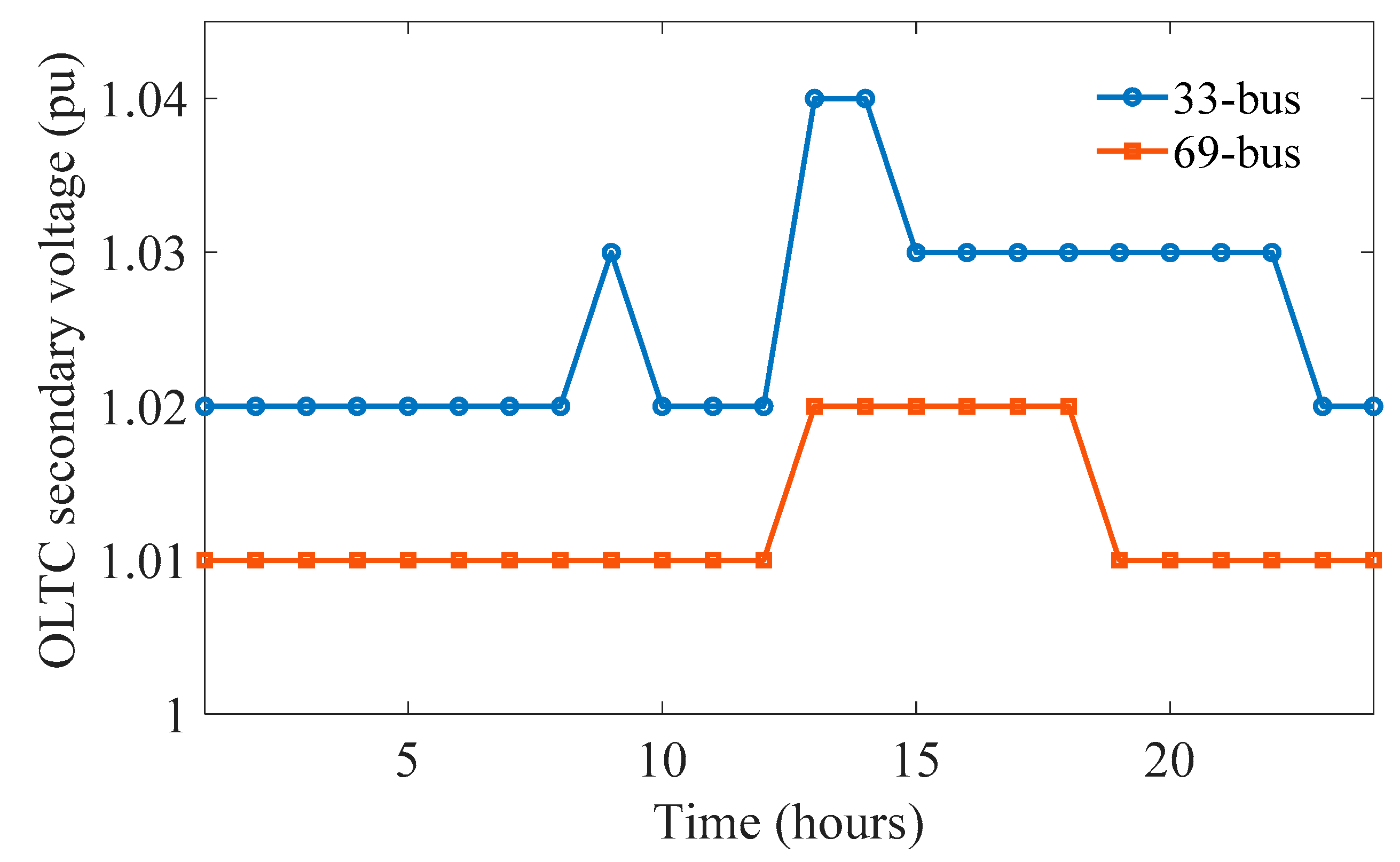
2.3.2. On Load Tap Changers
2.3.3. Capacitor Banks
2.3.4. Static Var Generator
2.3.5. Operating Constraints of Distributed Generations
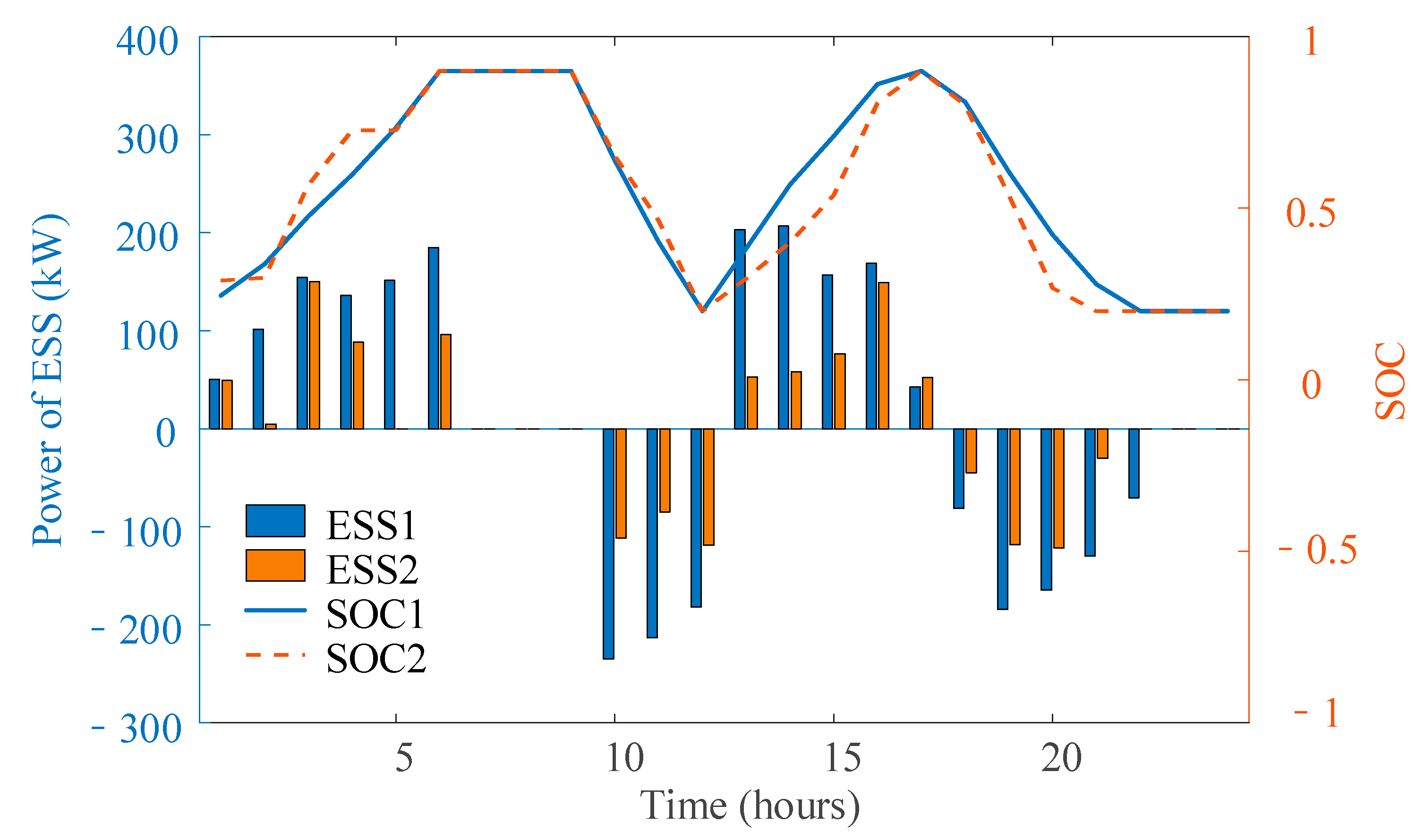
2.3.6. Energy Storage System
2.3.7. Security Constraints
3. Solution Method
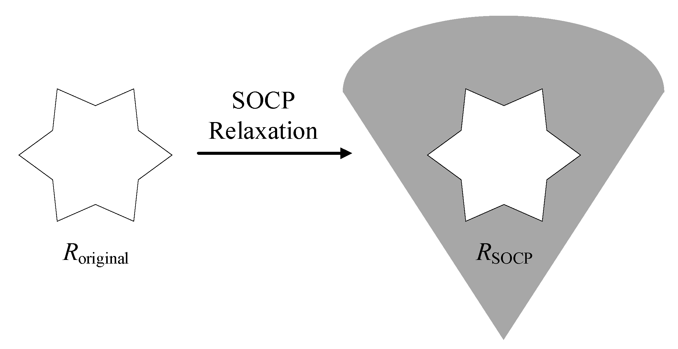
3.1. Brief Introduction of Second-Order Cone Programming and Second-Order Cone Programming Relaxation
3.2. Transformation of the Proposed Model
4. Case Studies
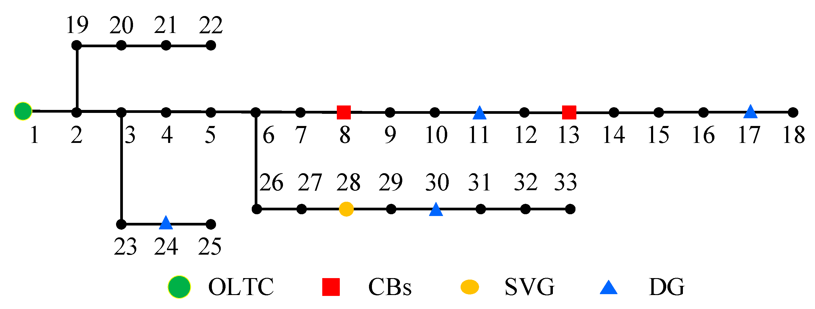
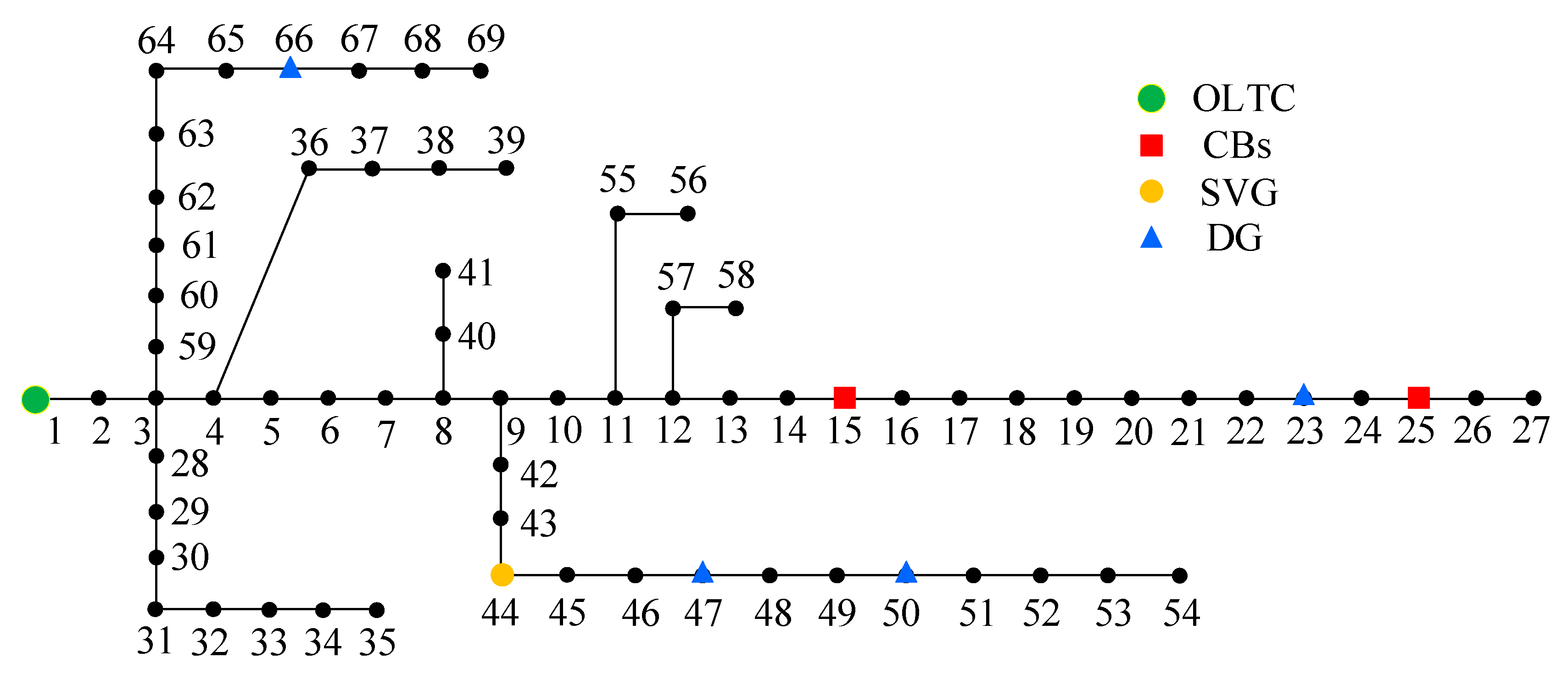
4.1. Basic Data
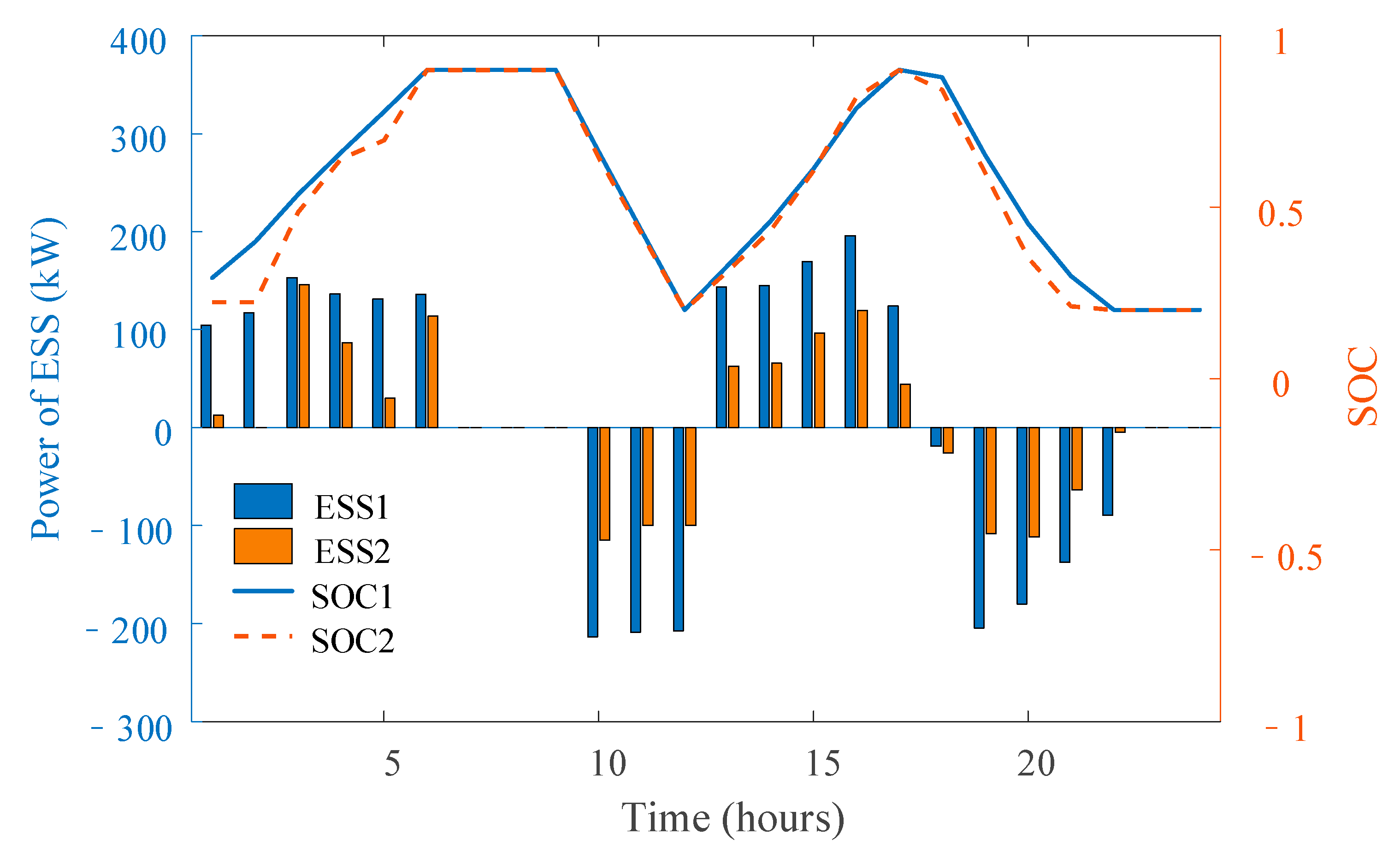
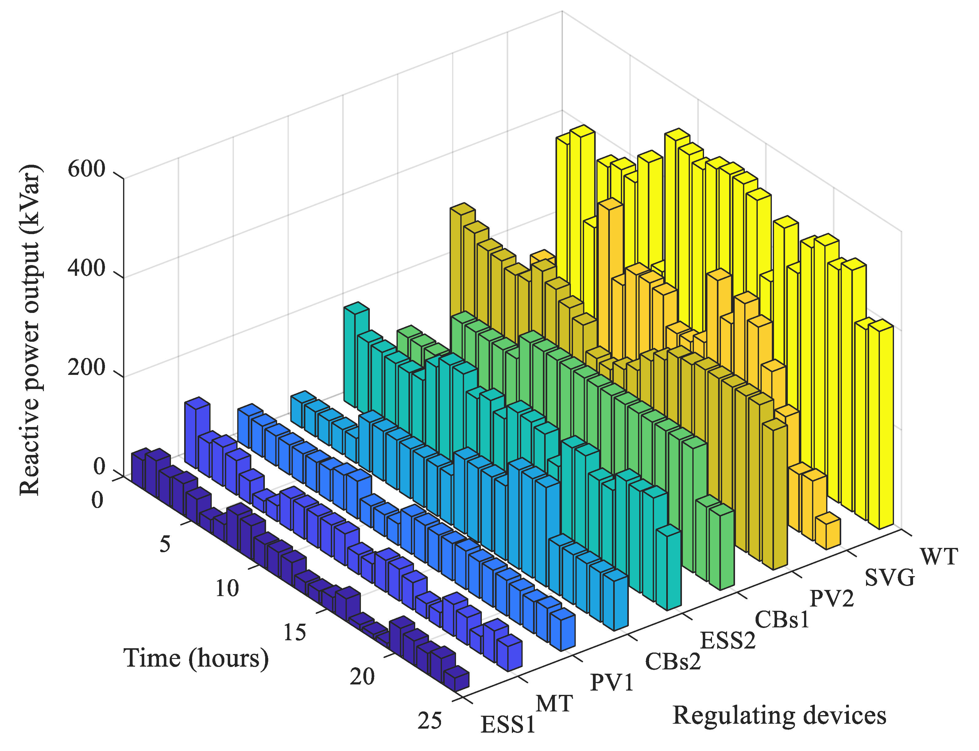
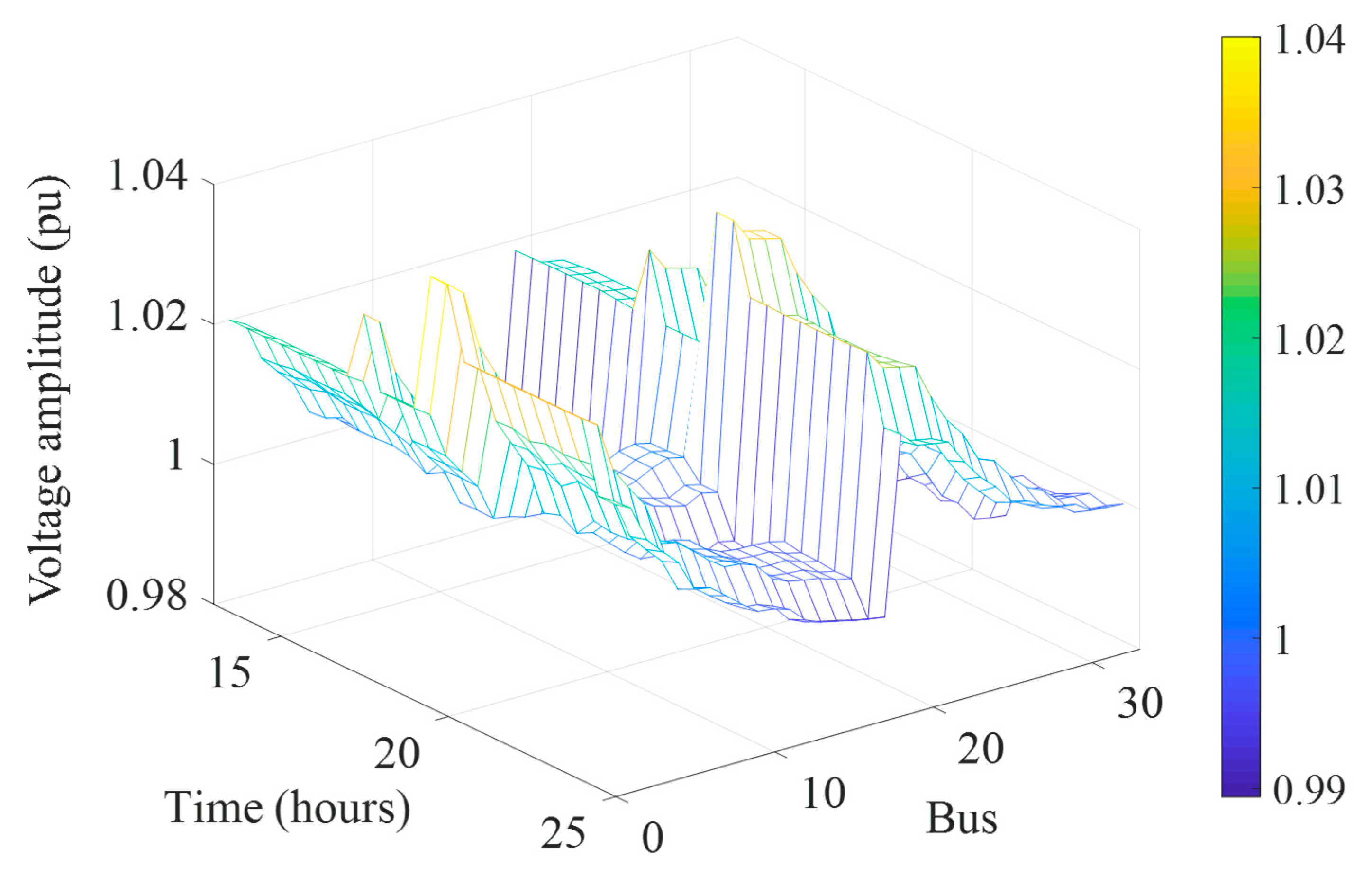
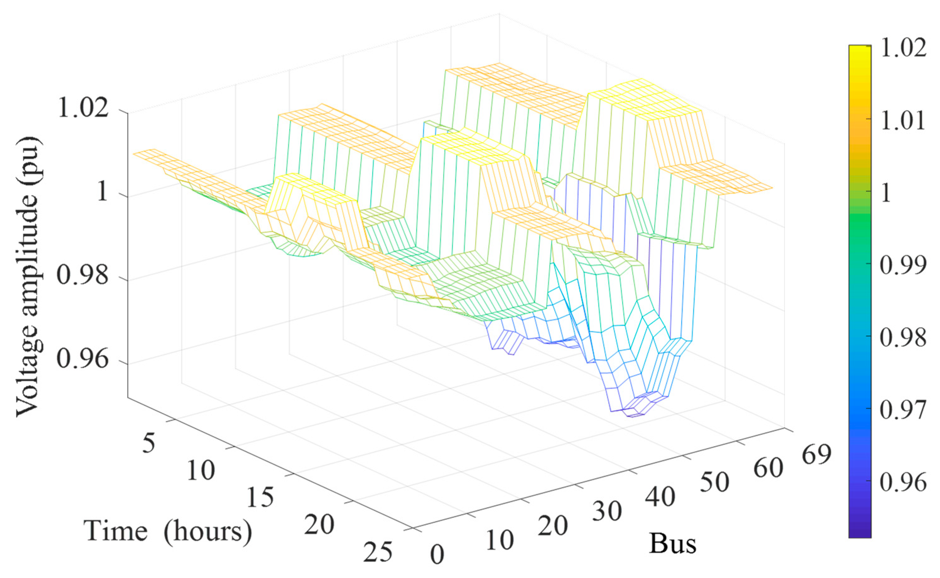
4.2. Optimization Results of the Proposed Model
4.3. Discussion
4.3.1. Comparison of Different Cases
4.3.2. Comparison of Different Methods
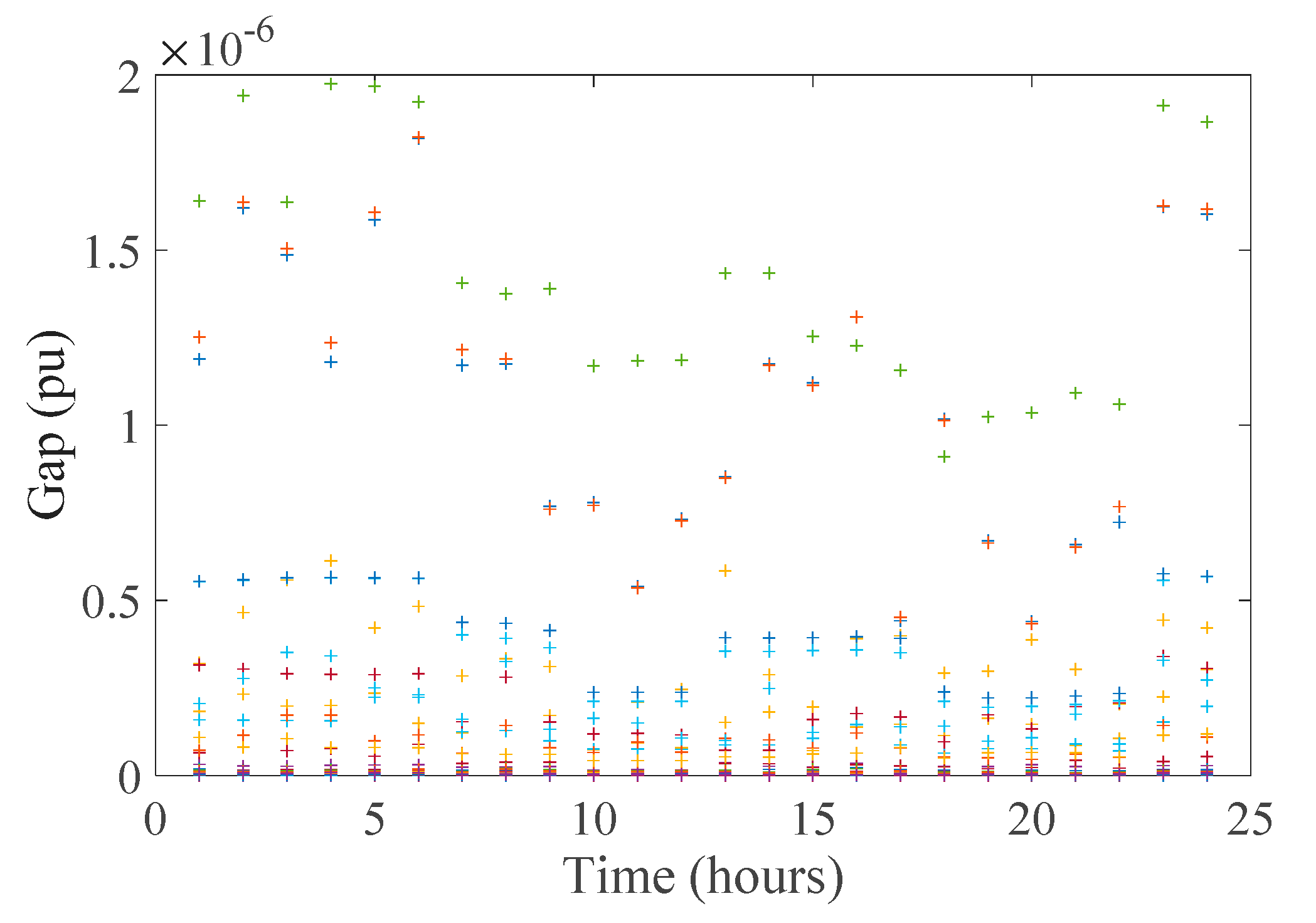
4.3.3. Relaxation Accuracy Analysis
5. Conclusions
Author Contributions
Funding
Conflicts of Interest
References
- Ding, T.; Bo, R.; Sun, H.B.; Li, F.X.; Guo, Q.L. A Robust Two–level coordinated static voltage security region for centrally integrated wind farms. IEEE Trans. Smart Grid 2017, 7, 460–470. [Google Scholar] [CrossRef]
- Elsaiah, S.; Benidris, M.; Mitra, J. An analytical approach for placement and sizing of distributed generators on power distribution system. IET Gener. Transm. Distrib. 2014, 8, 1039–1049. [Google Scholar] [CrossRef]
- Vita, V.; Alimardan, T.; Ekonomou, L. The impact of distributed generation in the distribution networks’ voltage profile and energy losses. In Proceedings of the 9th IEEE European Modelling Symposium on Mathematical Modelling and Computer Simulation, Madrid, Spain, 6–8 October 2015; IEEE: Piscataway, NJ, USA, 2015; pp. 260–265. [Google Scholar]
- Kaloudas, C.G.; Ochoa, L.F.; Marshall, B. Assessing the future trends of reactive power demand of distribution networks. IEEE Trans. Power Syst. 2017, 32, 4278–4288. [Google Scholar] [CrossRef]
- Chen, L.W.; Li, H.Y. Optimized reactive power supports using transformer tap stagger in distribution networks. IEEE Trans. Smart Grid 2017, 8, 1987–1996. [Google Scholar] [CrossRef]
- Hu, J.J.; Marinelli, M.; Coppo, M.; Zecchino, A.; Bindner, H.W. Coordinated voltage control of a decoupled three–phase on–load tap changer transformer and photovoltaic inverters for managing unbalanced networks. Electr. Power Syst. Res. 2016, 131, 264–274. [Google Scholar] [CrossRef]
- Fallahzadeh-Abarghouei, H.; Nayeripour, M.; Hasanvand, S. Online hierarchical and distributed method for voltage control in distribution smart grids. IET Gener. Transm. Distrib. 2016, 11, 1223–1232. [Google Scholar] [CrossRef]
- Keane, A.; Ochoa, L.F.; Borges, C.L.T.; Ault, G.W.; Alarcon-Rodriguez, A.D.; Currie, R.A.F.; Pilo, F.; Dent, C.; Harrison, G.P. State–of–the–art techniques and challenges ahead for distributed generation planning and optimization. IEEE Trans. Power Syst. 2013, 28, 1493–1502. [Google Scholar] [CrossRef]
- Coath, G.; Al-Dabbagh, M.; Halgamuge, S.K. Chaotic PSO–based VAR control considering renewables using fast probabilistic power flow. IEEE Trans. Power Deliv. 2014, 29, 1666–1674. [Google Scholar]
- Shaw, B.; Mukherjee, V.; Ghoshal, S.P. Solution of reactive power dispatch of power systems by an opposition–based gravitational search algorithm. Int. J. Electr. Power 2014, 55, 29–40. [Google Scholar] [CrossRef]
- Saraswat, A.; Saini, A.; Saxena, A.K. A novel multi–zone reactive power market settlement model: A pareto–optimization approach. Energy 2013, 51, 85–100. [Google Scholar] [CrossRef]
- Nguyen, T.T.; Dinh, B.H.; Quynh, N.V.; Duong, M.Q.; Dai, L.V. A novel algorithm for optimal operation of hydrothermal power systems under considering the constraints in transmission networks. Energies 2018, 11, 188. [Google Scholar] [CrossRef]
- Wei, H.; Sasaki, H.; Kubokawa, J.; Yokoyama, R. An interior point nonlinear programming for optimal power flow problems with a novel data structure. IEEE Trans. Power Syst. 1998, 13, 870–877. [Google Scholar] [CrossRef]
- Zheng, W.Y.; Wu, W.C.; Zhang, B.M.; Sun, H.B.; Liu, Y.B. A fully distributed reactive power optimization and control method for active distribution networks. IEEE Trans. Smart Grid 2014, 7, 1021–1033. [Google Scholar] [CrossRef]
- Mohamadreza, B.; Reza, H.M.; Mehrdad, G. Second–order cone programming for optimal power flow in VSC–type–AC–DC grids. IEEE Trans. Power Syst. 2013, 28, 4282–4291. [Google Scholar]
- Ding, T.; Cheng, L.; Li, F.X.; Chen, T.E.; Liu, R.F. A bi–objective DC–optimal power flow model using linear relaxation–based second order cone programming and its Pareto Frontier. Int. J. Electr. Power 2017, 88, 13–20. [Google Scholar] [CrossRef]
- Baradar, M.; Hesamzadeh, M.R. AC power flow representation in conic format. IEEE Trans. Power Syst. 2015, 30, 546–547. [Google Scholar] [CrossRef]
- Yang, Z.F.; Zhong, H.W.; Xia, Q.; Kang, C.Q. Solving OPF using linear approximations: Fundamental analysis and numerical demonstration. IET Gener. Transm. Distrib. 2017, 11, 4115–4125. [Google Scholar] [CrossRef]
- Cagnano, A.; De Tuglie, E.; Bronzini, M. Multiarea voltage controller for active distribution networks. Energies 2018, 11, 583. [Google Scholar] [CrossRef]
- Cagnano, A.; De Tuglie, E. A decentralized voltage controller involving PV generators based on Lyapunov theory. Renew. Energy 2016, 86, 664–674. [Google Scholar] [CrossRef]
- Duong, M.Q.; Sava, G.N. Coordinated reactive power control of DFIG to improve LVRT characteristics of FSIG in wind turbine generation. In Proceedings of the 2017 International Conference on Electromechanical and Power Systems (SIELMEN), Iasi, Romania, 11–13 October 2017; IEEE: Piscataway, NJ, USA, 2017; pp. 256–260. [Google Scholar]
- Shi, N.; Luo, Y. Bi–level programming approach for the optimal allocation of energy storage systems in distribution networks. Appl. Sci. 2017, 7, 398. [Google Scholar] [CrossRef]
- Zhang, Y.X.; Zhao, Y.D.; Luo, F.J.; Zheng, Y.; Meng, K.; Kit, P.W. Optimal allocation of battery energy storage systems in distribution networks with high wind power penetration. IET Renew. Power Gener. 2016, 10, 1105–1113. [Google Scholar] [CrossRef]
- Jiang, X.; Nan, G.L.; Liu, H.; Guo, Z.M.; Zeng, Q.S.; Jin, Y. Optimization of battery energy storage system capacity for wind farm with considering auxiliary services compensation. Appl. Sci. 2018, 8, 1957. [Google Scholar] [CrossRef]
- Bahramipanah, M.; Cherkaoui, R.; Paolone, M. Decentralized voltage control of clustered active distribution network by means of energy storage systems. Electr. Power Syst. Res. 2016, 136, 370–382. [Google Scholar] [CrossRef] [Green Version]
- Kabir, M.N.; Mishra, Y.; Ledwich, G. Coordinated control of grid connected photovoltaic reactive power and battery energy storage systems to improve the voltage profile of a residential distribution feeder. IEEE Trans. Ind. Inform. 2014, 10, 967–977. [Google Scholar] [CrossRef]
- Luo, F.; Meng, K.; Dong, Z.Y. Coordinated operational planning for wind farm with battery energy storage system. IEEE Trans. Sustain. Energy 2015, 6, 253–262. [Google Scholar] [CrossRef]
- Nieto, A.; Vita, V.; Maris, T.I. Power quality improvement in power grids with the integration of energy storage systems. Int. J. Eng. Res. Technol. 2016, 5, 438–443. [Google Scholar]
- Akhavan-Hejazi, H.; Mohsenian-Rad, H. Optimal operation of independent storage systems in energy and reserve markets with high wind penetration. IEEE Trans. Smart Grid 2014, 5, 1088–1097. [Google Scholar] [CrossRef]
- Chen, S.X.; Gooi, H.B.; Wang, M.Q. Sizing of energy storage for microgrids. IEEE Trans. Smart Grid 2012, 3, 142–151. [Google Scholar] [CrossRef]
- Rafiee Sandgani, M.; Sirouspour, S. Coordinated optimal dispatch of energy storage in a network of grid–connected microgrids. IEEE Trans. Sustain. Energy 2017, 8, 1166–1176. [Google Scholar] [CrossRef]
- Fan, H.; Yuan, Q.Q.; Cheng, H.Z. Multi–objective stochastic optimal operation of a grid–connected microgrid considering an energy storage system. Appl. Sci. 2018, 8, 2560. [Google Scholar] [CrossRef]
- Ding, T.; Liu, S.Y.; Wu, Z.Y.; Bie, Z.H. Sensitivity–based relaxation and decomposition method to dynamic reactive power optimization considering DGs in active distribution networks. IET Gener. Transm. Distrib. 2016, 11, 37–48. [Google Scholar] [CrossRef]
- Liu, Y.; Wu, W.C.; Zhang, B.M.; Li, Z.S.; Li, Z.G. A mixed integer second–order cone programming based active and reactive power coordinated multi–period optimization for active distribution network. Proc. Chin. Soc. Electr. Eng. 2014, 34, 2575–2583. [Google Scholar]
- Daratha, N.; Das, B.; Sharma, J. Coordination between OLTC and SVC for voltage regulation in unbalanced distribution system distributed generation. IEEE Trans. Power Syst. 2014, 29, 289–299. [Google Scholar] [CrossRef]
- Farivar, M.; Low, S.H. Branch flow model: Relaxations and convexification—Part I. IEEE Trans. Power Syst. 2013, 28, 2554–2564. [Google Scholar] [CrossRef]
- Farivar, M.; Low, S.H. Branch flow model: Relaxations and convexification—Part II. IEEE Trans. Power Syst. 2013, 28, 2565–2572. [Google Scholar] [CrossRef]
- Lee, C.; Liu, C.; Mehrotra, S.; Bie, Z.H. Robust distribution network reconfiguration. IEEE Trans. Smart Grid 2015, 6, 836–842. [Google Scholar] [CrossRef]
- Zhang, C.; Xu, Y.; Dong, Z.Y. Robust Coordination of distributed generation and price–based demand response in microgrids. IEEE Trans. Smart Grid 2018, 9, 4236–4247. [Google Scholar] [CrossRef]


| Location | DG Type | Rated Power (kW) |
|---|---|---|
| 11 | MT | 200 |
| 17 | PV1 | 300 |
| 24 | PV2 | 300 |
| 29 | WT | 500 |
| Type | State of Charge | |||||
|---|---|---|---|---|---|---|
| I | 1 | 0.3 | 0.5 | 0.9 | 0.9 | 0.2–0.9 |
| II | 0.5 | 0.15 | 0.2 | 0.9 | 0.9 | 0.2–0.9 |
| Type | Hours | Electricity Price (¥/kWh) |
|---|---|---|
| Peak period | 09:00–12:00, 17:00–22:00 | 1.15 |
| Flat period | 06:00–09:00, 12:00–17:00 | 0.68 |
| Valley period | 00:00–06:00, 22:00–24:00 | 0.33 |
| Case | 33-bus | 69-bus | ||||
|---|---|---|---|---|---|---|
| Before optimization | 2667.79 | 51,545.05 | 56.54 | 2951.03 | 53,129.68 | 62.80 |
| After optimization | 1144.56 | 47,798.40 | 13.94 | 1564.78 | 49,479.71 | 33.08 |
| Case | 33-bus Distribution Network | 69-bus Distribution Network | ||||
|---|---|---|---|---|---|---|
| Case 1 | 1388.95 | 48,819.63 | 17.08 | 2303.60 | 50,892.86 | 41.47 |
| Case 2 | 1383.71 | 48,001.09 | 16.20 | 2313.05 | 50,095.00 | 39.87 |
| Case 3 | 1173.97 | 48,635.31 | 15.29 | 1681.35 | 50,383.46 | 35.83 |
| Case 4 | 1144.56 | 47,798.40 | 13.94 | 1564.78 | 49,479.71 | 33.08 |
| Case | 33-bus Distribution Network | 69-bus Distribution Network | ||
|---|---|---|---|---|
| Objective | Computational Time (min) | Objective | Computational Time (min) | |
| Case 1 (MINLP) | 47,820.32 | >120 | 49,501.39 | >120 |
| Case 2 (MISOCP) | 47,788.41 | 5.13 | 49,469.17 | 9.08 |
© 2019 by the authors. Licensee MDPI, Basel, Switzerland. This article is an open access article distributed under the terms and conditions of the Creative Commons Attribution (CC BY) license (http://creativecommons.org/licenses/by/4.0/).
Share and Cite
Wang, L.; Wang, X.; Jiang, C.; Yin, S.; Yang, M. Dynamic Coordinated Active–Reactive Power Optimization for Active Distribution Network with Energy Storage Systems. Appl. Sci. 2019, 9, 1129. https://doi.org/10.3390/app9061129
Wang L, Wang X, Jiang C, Yin S, Yang M. Dynamic Coordinated Active–Reactive Power Optimization for Active Distribution Network with Energy Storage Systems. Applied Sciences. 2019; 9(6):1129. https://doi.org/10.3390/app9061129
Chicago/Turabian StyleWang, Lingling, Xu Wang, Chuanwen Jiang, Shuo Yin, and Meng Yang. 2019. "Dynamic Coordinated Active–Reactive Power Optimization for Active Distribution Network with Energy Storage Systems" Applied Sciences 9, no. 6: 1129. https://doi.org/10.3390/app9061129
APA StyleWang, L., Wang, X., Jiang, C., Yin, S., & Yang, M. (2019). Dynamic Coordinated Active–Reactive Power Optimization for Active Distribution Network with Energy Storage Systems. Applied Sciences, 9(6), 1129. https://doi.org/10.3390/app9061129