Identification of Coal Geographical Origin Using Near Infrared Sensor Based on Broad Learning

Abstract

Geographical origin, an important indicator of the chemical composition and quality grading, is one essential factor that should be taken into account in evaluating coal quality. However, traditional coal origin identification methods based on chemistry experiments are not only time consuming and labour intensive, but also costly. Near-Infrared (NIR) spectroscopy is an effective and efficient way to measure the chemical compositions of samples and has demonstrated excellent performance in various fields of quantitative and qualitative research. In this study, we employ NIR spectroscopy to identify coal origin. Considering the fact that the NIR spectra of coal samples always contain a large amount of redundant information and the number of samples is small, the broad learning algorithm is utilized here as the modelling system to classify the coal geographical origin. In addition, the particle swarm optimization algorithm is introduced to improve the structure of the Broad Learning (BL) model. We compare the improved model with the other five multivariate classification methods on a dataset with 243 coal samples collected from five countries. The experimental results indicate that the improved BL model can achieve the highest overall accuracy of 97.05%. The results obtained in this study suggest that the NIR technique combined with machine learning methods has significant potential for further development of coal geographical origin identification systems.

1. Introduction

Coal, as one of the most abundant primary fossil fuels, plays a critical role in meeting global energy needs and will remain important to humankind for many years to come [1]. It is highly desired to evaluate the coal quality for the rational use of coal. However, various factors can determine the quality of coal. Among them, one important aspect is its geographical origin [2,3]. The geographical origin can represent comprehensive factors including the climate, hydrology and minerals. The traditional coal geographical origin identification methods via chemistry experiments are complex and time consuming [4]. Meanwhile, some other rapid detection methods, such as gamma-ray-based methods [5] and microwave heating-based methods [6], focus on only a single property of coals (e.g., fixed carbon and moisture). Considering the limitations of previous methods, rapid, non-destructive, cost-effective analytical techniques for the coal geographical origin identification would be highly desirable [7,8]. In recent years, vibrational spectroscopy techniques along with the machine learning algorithms have been proven to be powerful tools in the analysis of fuel samples [9]. For instance, Wang et al. used Near-Infrared (NIR) spectroscopy with improved PLS regression for the rapid analysis of six coal properties [10]. Yang et al. identified coal and carbonaceous shale based on visible and NIR spectroscopy [11].

NIR spectroscopy is an effective and efficient technique to measure the chemical compositions of samples and has been widely used in the agricultural, petrochemical and pharmaceutical industries in the past few decades [12,13,14,15]. NIR has also been used to identify geographical origins. For example, Lin et al. used NIR spectroscopy and SPA-LDA simultaneously to classify the geographical origin and quality of tea [16]. Tony et al. classified the geographical origin of honey samples by NIR spectroscopy [17]. Gang-Feng Li et al. identified the adulterations and geographical origins of Chinese herbs by NIR spectroscopy and chemometrics [18]. Many traditional learning methods including Support Vector Machine (SVM) [19], Back Propagation Neural Network (BPNN) [20], Random Forest (RF) [21], etc., are combined with the NIR spectra to discriminate the geographical origin and quality of food and herbs [22]. However, compared with the NIR spectra of the above organics, there is more redundant information and noise in the NIR spectra of coal samples. Moreover, the data set is small, and inhomogeneity may exist. Considering the problems mentioned above, the traditional classification methods cannot meet the requirements of accurate and effective identification [23,24,25,26].

In this study, we employ a novel classification algorithm, Broad Learning (BL), which was recently proposed by Chen et al. [24]. BL is well known for its superior performance in solving several classification problems. Unlike the deep learning-based algorithms [27], there is no layer-to-layer coupling in the network structure. It has the advantage of a simple structure and low computational cost. The BL can be used in complex classification problems with less parameters to compute. Moreover, the incremental learning systems of BL can efficiently remodel the model in a broad, expansive way, and the retraining process is unnecessary if the network is deemed to be expanded. In order to further improve the performance of the BL model, we employ Particle Swarm Optimization (PSO) to optimize the structure of the BL model. Given its advantages of being powerful and easy to implement, the PSO algorithm has become universally applicable to various optimization problems [28]. Finally, we compare the proposed method with state-of-the-art methods in coal geographical origin identification. The results demonstrate that the proposed PSO-BL-based strategy achieves the best performance with an accuracy of 97.05%, which strengthens the contribution of the proposed method and further emphasizes the importance of the optimal parameters.

In this study, we propose a novel method to identify coal geographical origin. The main contributions of this paper are three-fold:

• Inspired by the usage of NIR in agriculture, petrochemical and pharmaceutical industries, we employ NIR to identify coal geographical origin, which is unprecedented. This method is fast and non-destructive.
• Considering the noisy NIR spectral and limited samples, we employ the BL as the modelling algorithm for its advantages of a simple structure, robustness to noise and excellent performance in previous studies. Compared with the traditional methods in the literature, this study improves the classification precision.
• The performance of BL is largely dependent on the network structure. In order to obtain the optimal parameters for the BL model, the PSO algorithm is utilized. The proposed method is able to classify the coal geographical origin accurately.

The rest of this paper is organized as follows. The experimental preparations, including the sources of data, data processing and outlier rejection, are presented in Section 1. Section 2 explains the theory of the BL model and presents the detail of our proposed PSO-BL model. Some comparison experiments are carried out to compare the performance of the PSO-BL model with that of the other five traditional discrimination methods, and the results are shown in Section 3. Section 4 concludes the whole paper.

2. Experimental Preparations

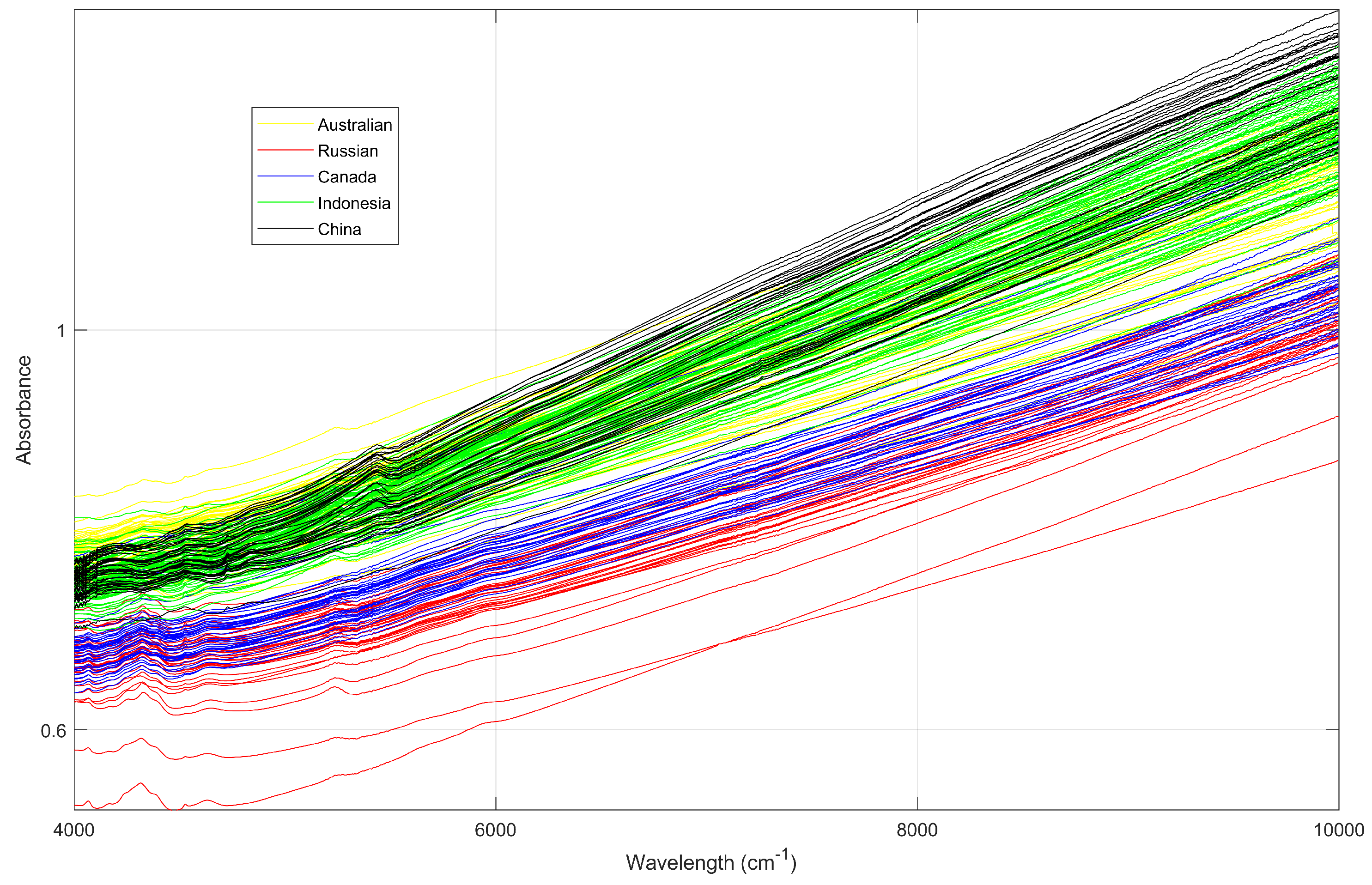
2.1. Experimental Data

We collected 243 coal samples from five countries, including 47 samples from Australia, 36 samples from Russia, 36 samples from Canada, 83 samples from Indonesia and 41 samples from China. Before spectra recording, all samples were prepared according to the “Method for Preparation of Coal Sample” (GB474-2008) [29] by using a KERP hammer crusher, an SF-05 automatic sample splitter, and a 0.2 mm-standard sieve in the National Laboratory of the Import and Export Quarantine Inspection Bureau. Prior to the measurement of each sample’s spectrum, we measured the background spectrum, the response of the spectrometer when there was no sample in place. Then, we utilized the background spectrum to eliminate signals due to the spectrometer and its environment. Therefore, the final spectrum was due solely to the sample. Then, the prepared coal samples were scanned by an Antaris II FT-NIR Spectrometer (Thermo Electron Co., Waltham, MA, USA) in the range of 10,001.00–3999.64 cm${}^{-1}$, and in total, we obtained 1557 wavelength points. Each sample spectrum was scanned 64 times, and the spectrum of each sample was the average of 64 scans performed at a resolution of 4 cm${}^{-1}$. The near-infrared spectrum of the coal samples is shown in Figure 1. As can be seen from Figure 1, the NIR spectra consists of broad, weak and extensively-overlapping bands, which may impede further analysis. In order to identify coal geographical origins, it is of great necessity to employ powerful machine learning algorithms that are robust to noise.

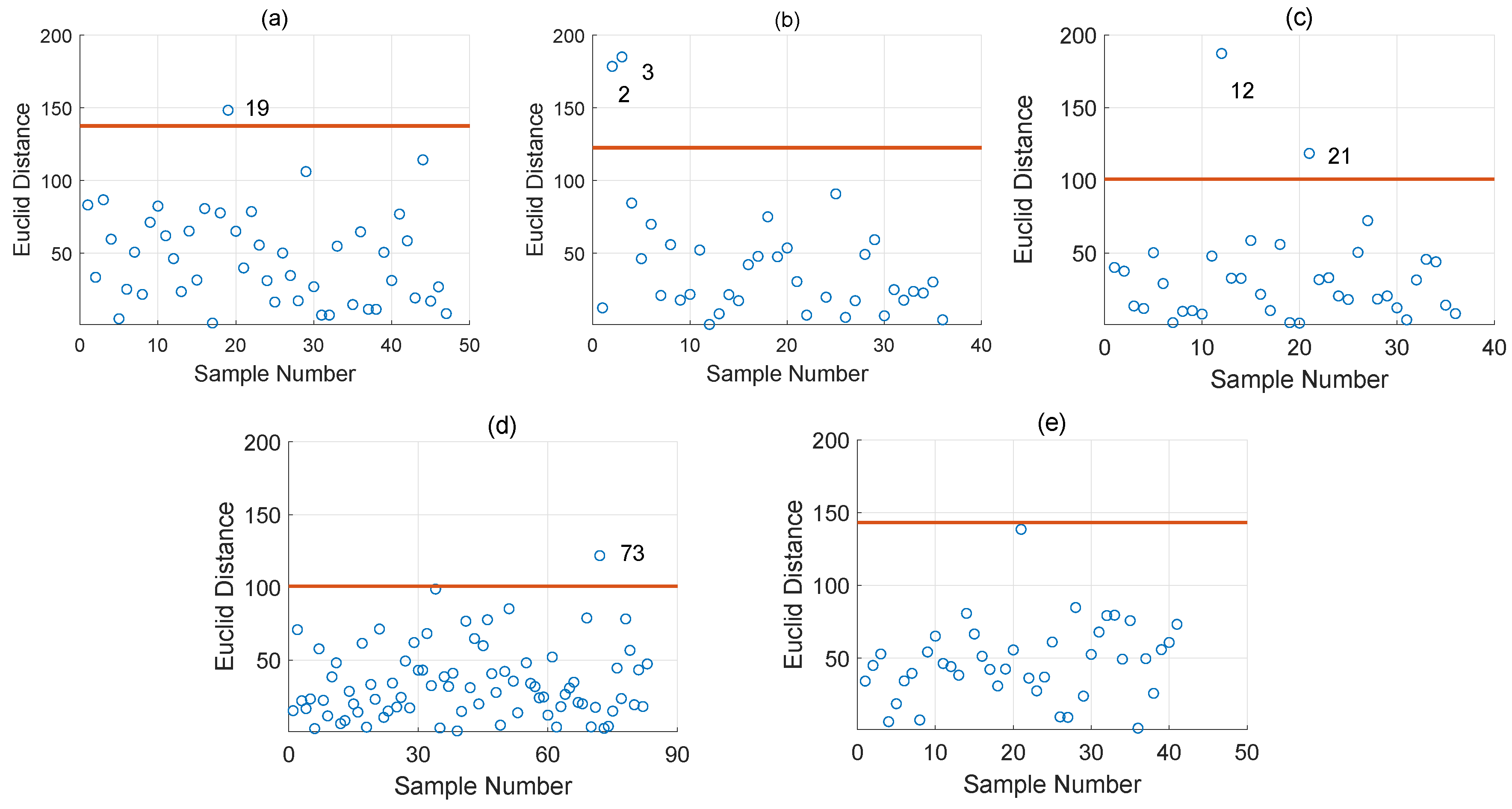
2.2. Outlier Rejection

In practice, experimental data often contain outliers, which are different from the majority. During the spectral data collection, outliers might be due to the environmental influence and incorrect operating. However, commonly-used machine learning methods are sensitive to such outliers, and the results may be adversely affected by them [30]. Therefore, it is of great importance to detect and reject these outliers. In this paper, the outliers are detected according to the Euclidean distance (Ed) between samples with the centres. First, we calculate the average spectrum of samples from each country, denoted as the central vector,

$$\begin{array}{c}\hfill \overline{X}=\frac{1}{\#s}\sum _{s=1}^{\#s}{X}_s,\end{array}$$

(1)

where $\#s$ is the number of samples in each country. Then, we calculate the average of the Euclidean distances between the spectra of each coal sample and the central vector:

$$\begin{array}{c}\hfill dis=\frac{1}{\#s}\sum _{s=1}^{\#s}\sqrt{{(X_s-\overline{X})}^2}.\end{array}$$

(2)

To detect the outliers, the threshold is set as $3\times dis$. The sample is regarded as an outlier when the Euclidean distance between the coal sample and $\overline{X}$ is larger than the threshold. The results of the outlier rejection are shown in Figure 2. It can be found that the samples whose indexes are 12 in Australia, 2 and 3 in Russia, 12 and 21 in Canada and 73 in Indonesia are eliminated from the data set. We also employed the Hotelling T-squared [31] to remove the outliers, and similar results were achieved.

3. Experimental Methods

3.1. BL Algorithm

BL is based on the Random Vector Functional-link Neural Network (RVFLNN) previously proposed in [32]. Instead of gradient-descent-based learning algorithms [33], RVFLNN provides the generalization capability as a function approximation by calculating the pseudoinverse to find the desired connection weights. However, RVLNN does not work well in the modern large data era. Chen et al. proposed a novel strategy, namely broad learning, which is able to cope with the new incoming data [24]. As shown in Figure 3, there are four parts of a BL network, including input, output, feature nodes and enhancement nodes. In the BL model, the input data are first mapped into a series of random feature nodes, similar to the feature extraction process in traditional machine learning. After that, the mapped random feature nodes are transformed into enhancement nodes by a nonlinear transformation. Further, we connect the output label with the combination of mapped feature nodes and enhancement nodes, and the connection weight W is the learning parameter, which can be calculated by ridge regression [34].

Given a dataset $(X,Y)$ with N samples where X are the input data and Y is the output label, the algorithm implementation process is as follows: We first transform the input data X into the mapped random features $Z_i, i=1,\dots ,n$, where n is the number of mapped features. The $i^{\mathrm{th}}$ mapped feature node is:

$$\begin{array}{c}\hfill Z_i={\varphi }_i(X{W}_{e_i}+b_{e_i}), i=1,\dots ,n,\end{array}$$

(3)

where $W_{e_i}$ and $b_{e_i}$ are the random weights and bias and ${\varphi }_i(·)$ is the mapping function. Then, we denote $Z^{*}\stackrel{\Delta }{=}(Z_1,Z_2,\dots ,Z_n)$ as the outputs of n feature nodes. In order to obtain sparse and compact features of $Z^{*}$, we fine-tune the initialized weights $W_{e_i}$ by using a sparse autoencoder. After obtaining the mapped feature nodes, $Z^{*}$ is input into the enhancement nodes $H_j, j=1,\dots ,m$ where m is the number of enhancement nodes. The $j^{\mathrm{th}}$ enhancement nodes can be calculated as:

$$\begin{array}{c}\hfill H_j={\delta }_j(Z^{*}{W}_{h_j}+{\beta }_{h_j}),j=1,\dots ,m,\end{array}$$

(4)

where $W_{h_j}$ and ${\beta }_{h_j}$ are the random weights and bias and ${\delta }_j(·)$ is the active function chosen as $tanh(·)$ here. We define the outputs of enhancement nodes as $H^{*}\stackrel{\Delta }{=}(H_1,H_2,\dots ,H_m)$. Hence, the algorithm of BL can be described as:

$$\begin{array}{c}\hfill Y=[Z_1,Z_2,\dots ,Z_n|H_1,H_2,\dots ,H_m]W=\left[Z^{*}\right|H^{*}]W\end{array}$$

(5)

where $\left[Z^{*}\right|H^{*}]$ is the total feature nodes and W is the desired connection weight matrix between the feature nodes and the output label. By taking $A=\left[Z^{*}\right|H^{*}]$, Formula (5) can be represented as $Y=AW$. The BL aims to calculate the W through ridge regression approximation [34] as the following minimization problem:

$$\begin{array}{c}\hfill \underset{W}{min}\left|\right|Y-{AW\left|\right|}_2^2+{\lambda \left|\right|W\left|\right|}_2^2,\end{array}$$

(6)

where $\lambda$ is a positive constant to avoid over-fitting. We calculate the partial derivation of Formula (6) with respect to W and set the derivation to be zero. Then, we can get the W as:

$$\begin{array}{c}\hfill W={(\lambda I+A{A}^T)}^{-1}{A}^{T}Y.\end{array}$$

(7)

Then, we can find the desired connection weights.

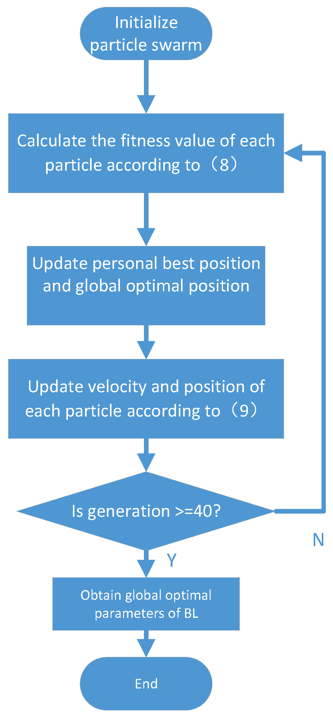
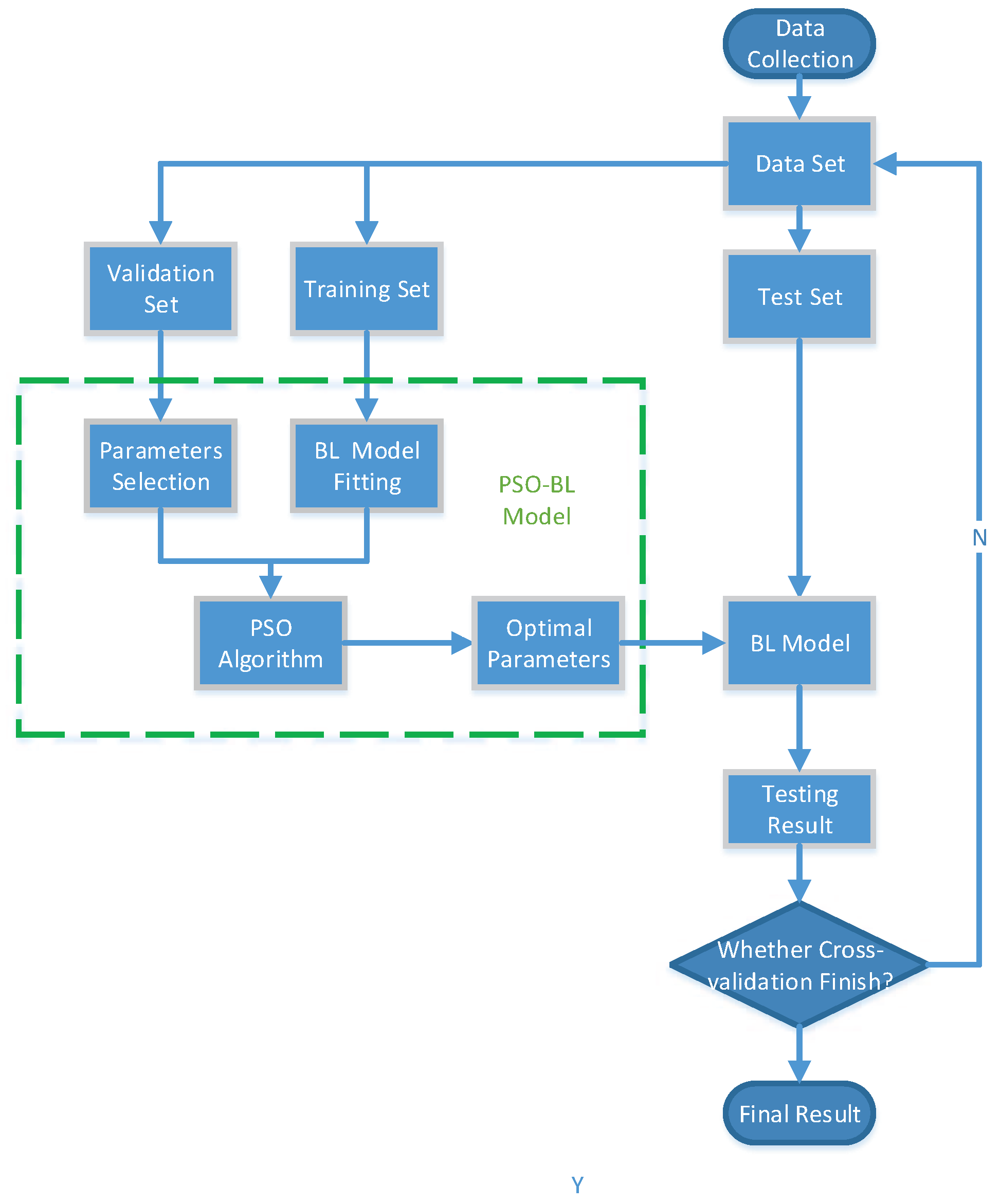
3.2. Proposed PSO-BL Model

The BL model is significantly affected by the relevant parameters of its structure. Hence, in order to improve the performance of the BL model, we employ the PSO algorithm to search for the optimal parameters. PSO is a classic global optimization strategy that is based on the flocking behaviour and social co-operation of birds [35]. In this experiment, we denote $N_1$ as the number of windows for feature mapping, $N_2$ as the number of nodes in each window and $N_3$ as the number of enhancement nodes. During the BL model construction, we find that the classification performance is largely dependent on the selection of these three parameters, $N_1$, $N_2$ and $N_3$. The PSO algorithm is applied here to obtain the optimal values of these three parameters. The fitness function of the optimization process is defined as follows,

$$\begin{array}{c}\hfill f_{fitness}=\frac{1}{10}\sum _{k=1}^{10}b{l}_k[n_1,n_2,n_3],\end{array}$$

(8)

where $b{l}_k[n_1,n_2,n_3]$ is the test accuracy of the $k^{\mathrm{th}}$ BL model when the parameters equal $n_1,n_2,n_3$. In order to reduce the random error, we calculate the BL model 10 times and return the mean of the accuracy as the fitness value. Figure 4 demonstrates the optimization process of the proposed BL with PSO. During the PSO optimization process, we initialize a swarm of 50 particles. In this study, the dimension of parameters’ particles d is set as three, which represents the number of parameters to optimize. We denote $p_{best,h}^d\left(t\right)$ as the best solution that particle h has obtained until generation t, and $p_{gbest}^d\left(t\right)$ is the best solution of all particles. Similarly, the velocity $V_h^d\left(t\right)$ and $X_h^d\left(t\right)$ denote that the velocity and position of the particle h have obtained generation t. In our study, it should be noted that the optimal parameters are the number of mapping features and enhancement nodes, which must be a positive integer. Similarly, the optimal velocity is also an integer. In each generation, we update velocity by the following formula,

$$\begin{array}{c}\hfill \begin{array}{cc}\hfill V_h^d(t+1)=& round[w{v}_h^d\left(t\right)+c_1{r}_1(p_{best,h}^d\left(t\right)-p_h^d)+\hfill \\ & c_2{r}_2(p_{gbest}^d\left(t\right)-p_h^d\left(t\right)]\hfill \end{array}\end{array}$$

(9)

where $r_1$ and $r_2$ are random numbers between [0,1] and $c_1$, $c_2$ are two positive acceleration constants chosen as 1.4962, which is commonly selected in the PSO algorithm. The $round$ is the function to round the number to the nearest integer. w is the dynamic inertia weight, which is expressed as:

$$\begin{array}{c}\hfill w=w_{max}-(w_{max}-w_{min})\ast {(t/M)}^2,\end{array}$$

(10)

where $w_{max}=0.9$, $w_{min}=0.25$, t is the current generation and M is the max generations, which equals 40. The position is updated as follows,

$$\begin{array}{c}\hfill p_h^d(t+1)=p_h^d\left(t\right)+V_h^d\left(t\right).\end{array}$$

(11)

During the optimal process, we heuristically assume that the velocity $V_h^d$ when $d=1,\dots ,3$ is in the range of $[-10,10]$, $[-10,10]$ and $[1000,-1000]$, respectively, the corresponding position $p_h^d$ is in the range of $[1,50]$, $[1,50]$ and $[10,10,000]$. The major steps of the proposed PSO-BL algorithm are summarized in Algorithm 1.

Algorithm 1: The proposed PSO-BL algorithm.

4. Results and Discussion

4.1. Model Construction

This section presents the model construction and the design of the experiment. After rejecting six outliers, we had 237 samples remaining. During the PSO-BL mode, we first divided the 237 samples into the training data set, the validation data set and the test data set. To improve the stability of the BL model and use the data more efficiently, 10-fold cross-validation was employed here. The total data set was split into 10 parts. Eight parts was applied in the training process of the BL model, and one part was utilized as the validation data to return the fitness value of the given parameters. The remaining part was used as the test data set to evaluate the performance of the PSO-BL model. The program was run 10 times, and each sample was given the opportunity to be used in the hold-out test set. The modelling process of the PSO-BL model is shown in Figure 5.

To improve the predictive ability of the BL system, in this study, we employed the PSO algorithm to optimize the construction of the BL network. The fitness value of the initial population is shown in Figure 6, where the swarm size is 50. It can be seen from Figure 6 that the fitness value of the initial population was mostly in the range of [0.84 0.96]. The performance was largely dependent on the value of the parameters. As mentioned above, 10-fold cross-validation was employed here. Hence, we repeated the experiment 10 times, and the global optimal fitness values of these 10 iterations are shown in Figure 7.

Table 1. Results of the PSO-BL model on the test set.

Times	1	2	3	4	5	6	7	8	9	10
Accuracy	1	0.917	0.958	0.958	1	1	1	0.913	1	0.957

demonstrates the process of cross-validation and shows the performance on 10 different test sets. We also calculate the accuracy corresponding to each region (i.e., five countries). As shown in

Table 2. Classification results of different methods.

Method	Index	Geographical Origin					Overall Accuracy
		AUS	RUS	CAN	IND	CHN
SVM	misclassification	6	4	5	2	2	92.83%
	accuracy	87.0%	88.2%	85.3%	97.6%	95.1%
BPNN	misclassification	5	3	5	5	0	92.40%
	accuracy	89.1%	91.2%	85.3%	93.9%	100%
RBFNN	misclassification	4	5	6	2	1	92.40%
	accuracy	91.2%	85.3%	82.4%	97.6%	97.6%
K-NN	misclassification	6	6	8	18	12	78.90%
	accuracy	87.0%	82.4%	76.5%	78.0%	70.7%
RF	misclassification	7	7	9	13	9	81.01%
	accuracy	84.8%	79.4%	73.5%	84.1%	78.0%
BL	misclassification	2	1	4	3	0	95.78%
	accuracy	95.7%	97.1%	88.2%	96.3%	100%
PSO-BL	misclassification	1	1	1	3	1	97.05%
	accuracy	97.8%	97.1%	97.1%	96.3%	97.6%

, the PSO-BL model totally misclassified seven samples and achieved the state-of-the-art performance of 97.05%. We also evaluated the performance of the proposed PSO-BL algorithm without outlier rejection, and the corresponding accuracy was 91.88%, significantly lower than that of the scheme with outlier removal.

Furthermore, we compared the proposed PSO-BL method with six traditional machine learning methods to identify the geographical origin of coal samples, including SVM, K-Nearest Neighbour (K-NN) [36], Radial Basis Function Neural Network (RBFNN) [37], the BPNN algorithm, RF and the BL model. Principal components analysis was employed to reduce the dimension and hence to enhance the computational efficiency of the SVM model. Moreover, the PSO algorithm was also used to obtain the optimal two parameters of the SVM model, namely c and $gamma$ of the RBF kernel SVM.

4.2. Experiment Results

The classification results of all the above-mentioned machine learning methods are shown in Table 2. BL, SVM, RBFNN and BPNN performed better than the other traditional classification methods, and the proposed PSO-BL achieved the highest accuracy of 97.05%. The comparison results demonstrate the effectiveness of the proposed PSO-BL algorithm, strengthen its contribution and further consolidate the necessity of the optimal parameters.

In addition, as can be seen from Table 2, the models had better performance on the samples of Indonesia and China. We suspect the potential reason was in two-fold. First, the samples set was imbalanced, resulting in a better classification with the bigger sample set. Moreover, the coal samples from Australia, Russia and Canada were mostly lignite, and the coal samples from China and Indonesia were mostly gas coal. Therefore, it can be inferred that the NIR spectroscopy had a better classification performance of coal geographical origin for the gas coal.

5. Conclusions

In this study, a novel method based on NIR spectra was proposed for fast and non-destructive identification of coal geographical origin. We employed the BL algorithm as the modelling method due to its advantages of a simple structure, low computational cost, as well as its excellent performance. In order to further improve the predictive ability of the BL model, the PSO algorithm was utilized to optimize the structure of the BL model. In addition, we compared the proposed PSO-BL model with the other six different multivariate classification methods, including SVM, K-NN, RBFNN, BPNN, RF, as well as BL. The experimental results indicated that the proposed PSO-BL model was superior to previous approaches, achieving the best classification accuracy of 97.05% with 10-fold cross-validation. In general, the proposed PSO-BL based method can identify the geographical origin of coal effectively and efficiently. The established protocol is of great importance to evaluate coal quality.

References

1. Vassilev, S.V.; Vassileva, C.G.; Vassilev, V.S. Advantages and disadvantages of composition and properties of biomass in comparison with coal: An overview. Fuel 2015, 158, 330–350. [Google Scholar] [CrossRef]
2. Meng, Z.P.; Liu, C.L.; Yi-Ming, J.I. Geological conditions of coalbed methane and shale gas exploitation and their comparison analysis. J. Coal Sci. Eng. 2013, 38, 728–736. [Google Scholar]
3. Li, D.; Li, Z.; Li, W.; Liu, Q.; Feng, Z.; Fan, Z. Hydrotreating of low temperature coal tar to produce clean liquid fuels. J. Anal. Appl. Pyrolysis 2013, 100, 245–252. [Google Scholar] [CrossRef]
4. Sajdak, M.; Stelmach, S.; Kotyczka-Morańska, M.; Plis, A. Application of chemometric methods to evaluate the origin of solid fuels subjected to thermal conversion. J. Anal. Appl. Pyrolysis 2015, 113, 65–72. [Google Scholar] [CrossRef]
5. Galper, A.M.; Adriani, O.; Aptekar, R.L.; Arkhangelskaja, I.V.; Arkhangelskiy, A.I.; Avanesov, G.A.; Bergstrom, L.; Bogomolov, E.A.; Boezio, M.; Bonvicini, V. The space-based gamma-ray telescope GAMMA-400 and its scientific goals. arXiv, 2013; arXiv:1306.6175. [Google Scholar]
6. Xia, W.; Yang, J.; Liang, C. A short review of improvement in flotation of low rank/oxidized coals by pretreatments. Powder Technol. 2013, 237, 1–8. [Google Scholar] [CrossRef]
7. Mastalerz, M.; He, L.; Melnichenko, Y.B.; Rupp, J.A. Porosity of coal and shale: Insights from gas adsorption and SANS/USANS techniques. Energy Fuels 2012, 26, 5109–5120. [Google Scholar] [CrossRef]
8. Kinnon, E.C.P.; Golding, S.D.; Boreham, C.J.; Baublys, K.A.; Esterle, J.S. Stable isotope and water quality analysis of coal bed methane production waters and gases from the Bowen Basin, Australia. Int. J. Coal Geol. 2010, 82, 219–231. [Google Scholar] [CrossRef]
9. Balabin, R.M. Near-infrared (NIR) spectroscopy for biodiesel analysis: Fractional composition, iodine value, and cold filter plugging point from one vibrational spectrum. Energy Fuels 2011, 25, 2373–2382. [Google Scholar] [CrossRef]
10. Wang, Y.; Yang, M.; Wei, G.; Hu, R.; Luo, Z.; Li, G. Improved PLS regression based on SVM classification for rapid analysis of coal properties by near-infrared reflectance spectroscopy. Sens. Actuators B Chem. 2014, 193, 723–729. [Google Scholar] [CrossRef]
11. Yang, E.; Ge, S.; Wang, S. Characterization and identification of coal and carbonaceous shale using visible and near-infrared reflectance spectroscopy. J. Spectrosc. 2018, 2018. [Google Scholar] [CrossRef]
12. Zhang, J.; Feng, X.; Liu, X.; He, Y. Identification of hybrid okra seeds based on near-infrared hyperspectral imaging technology. Appl. Sci. 2018, 8, 1793. [Google Scholar] [CrossRef]
13. Hu, Y.; Zou, L.; Huang, X.; Lu, X. Detection and quantification of offal content in ground beef meat using vibrational spectroscopic-based chemometric analysis. Sci. Rep. 2017, 7, 15162. [Google Scholar] [CrossRef] [PubMed]
14. Roberts, J.; Power, A.; Chapman, J.; Chandra, S.; Cozzolino, D. A short update on the advantages, applications and limitations of hyperspectral and chemical imaging in food authentication. Appl. Sci. 2018, 8, 505. [Google Scholar] [CrossRef]
15. Zhu, Z.; Yuan, H.; Song, C.; Li, X.; Fang, D.; Guo, Z.; Zhu, X.; Liu, W.; Yan, G. High-speed sex identification and sorting of living silkworm pupae using near-infrared spectroscopy combined with chemometrics. Sens. Actuators B Chem. 2018, 268, 299–309. [Google Scholar] [CrossRef]
16. Lin, H.; Zhao, J.; Chen, Q.; Zhou, F.; Sun, L. Discrimination of Radix Pseudostellariae according to geographical origins using NIR spectroscopy and support vector data description. Spectrochim. Acta Part A Mol. Biomol. Spectrosc. 2011, 79, 1381–1385. [Google Scholar] [CrossRef] [PubMed]
17. Tony, W.; Gerard, D.; Daniel, J.K.; Colm, O. Geographical classification of honey samples by near-infrared spectroscopy: A feasibility study. J. Agric. Food Chem. 2007, 55, 9128–9134. [Google Scholar]
18. Li, G.F.; Yin, Q.B.; Zhang, L.; Kang, M.; Fu, H.Y.; Cai, C.B.; Xu, L. Fine classification and untargeted detection of multiple adulterants of Gastrodia elata BI.(GE) by near-infrared spectroscopy coupled with chemometrics. Anal. Methods 2017, 9, 1897–1904. [Google Scholar] [CrossRef]
19. Joachims, T. Making large-scale svm learining practical. Adv. Kernel Methods Support Vector Learn. 2006, 8, 499–526. [Google Scholar]
20. Al-kaf, H.A.G.; Chia, K.S.; Alduais, N.A.M. A comparison between single layer and multilayer artificial neural networks in predicting diesel fuel properties using near infrared spectrum. Pet. Sci. Technol. 2018, 36, 411–418. [Google Scholar] [CrossRef]
21. Zou, L.; Huang, Q.; Li, A.; Wang, M. A genome-wide association study of Alzheimer’s disease using random forests and enrichment analysis. Sci. China Life Sci. 2012, 55, 618–625. [Google Scholar] [CrossRef] [PubMed]
22. Ribeiro, L.D.S.; Gentilin, F.A.; Franca, J.A.D.; Franca, M.B.D.M. Development of a hardware platform for detection of milk adulteration based on near-infrared diffuse reflection. IEEE Trans. Instrum. Meas. 2016, 65, 1698–1706. [Google Scholar] [CrossRef]
23. Zhao, L.; Chen, Z.; Yang, L.T.; Deen, M.J.; Wang, Z.J. Deep semantic mapping for heterogeneous multimedia transfer learning co-occurrence data. ACM Trans. Multimed. Comput. Commun. Appl. (TOMM) 2019, 15, 9. [Google Scholar] [CrossRef]
24. Chen, C.L.P.; Liu, Z. Broad learning system: An effective and efficient incremental learning Ssystem without the need for deep architecture. IEEE Trans. Neural Netw. Learn. Syst. 2017, 29, 10–24. [Google Scholar] [CrossRef] [PubMed]
25. Moreira, M.; França, J.A.D.; Filho, D.D.O.T.; Beloti, V.; Yamada, A.K.; França, M.B.D.M.; Ribeiro, L.D.S. A low-cost NIR digital photometer based on InGaAs Ssensors for the detection of milk adulterations with water. IEEE Sens. J. 2016, 16, 3653–3663. [Google Scholar] [CrossRef]
26. Zou, L.; Zheng, J.; Miao, C.; Mckeown, M.J.; Wang, Z.J. 3D CNN based automatic diagnosis of attention deficit hyperactivity disorder using functional and structural MRI. IEEE Access 2017, 5, 23626–23636. [Google Scholar] [CrossRef]
27. Lecun, Y.; Bengio, Y.; Hinton, G. Deep learning. Nature 2015, 521, 436. [Google Scholar] [CrossRef] [PubMed]
28. Pluhacek, M.; Senkerik, R.; Davendra, D.; Oplatkova, Z.K.; Zelinka, I. On the behaviour and performance of chaos driven PSO algorithm with inertia weight. Comput. Math. Appl. 2013, 66, 122–134. [Google Scholar] [CrossRef]
29. Li, T.; Dai, S.F.; Zou, J.H.; Zhang, S.; Tian, H.H.; Zhao, L.X. Composition and mode of occurrence of minerals in Late Permian coals from Zhenxiong County, northeastern Yunnan, China. Int. J. Coal Sci. Technol. 2014, 1, 13–22. [Google Scholar] [CrossRef]
30. Rousseeuw, P.J.; Debruyne, M.; Engelen, S.; Hubert, M. Robustness and outlier detection in chemometrics. Crit. Rev. Anal. Chem. 2006, 36, 221–242. [Google Scholar] [CrossRef]
31. Shan, J.; Suzuki, T.; Suhandy, D.; Ogawa, Y.; Kondo, N. Chlorogenic acid (CGA) determination in roasted coffee beans by Near Infrared (NIR) spectroscopy. Eng. Agric. Environ. Food 2014, 7, 139–142. [Google Scholar] [CrossRef]
32. Pao, Y.H.; Takefuji, Y. Functional-link net computing: Theory, system architecture, and functionalities. Computer 1992, 25, 76–79. [Google Scholar] [CrossRef]
33. Nair, M.V.; Dudek, P. Gradient-descent-based learning in memristive crossbar arrays. In Proceedings of the International Joint Conference on Neural Networks, Killarney, Ireland, 11–16 July 2015. [Google Scholar]
34. Mcdonald, G.C. Tracing ridge regression coefficients. Wiley Interdiscip. Rev. Comput. Stat. 2010, 2, 695–703. [Google Scholar] [CrossRef]
35. Liu, B.; Wang, L.; Jin, Y.H. An effective PSO-based memetic algorithm for flow shop scheduling. IEEE Trans. Syst. Man Cybern. Part B. 2007, 37, 18–27. [Google Scholar] [CrossRef]
36. Bijalwan, V.; Kumar, V.; Kumari, P.; Pascual, J. KNN based machine learning approach for text and document mining. Int. J. Database Theory Appl. 2014, 7, 61–70. [Google Scholar] [CrossRef]
37. Aljarah, I.; Faris, H.; Mirjalili, S.; Al-Madi, N. Training radial basis function networks using biogeography-based optimizer. Neural Comput. Appl. 2018, 29, 529–553. [Google Scholar] [CrossRef]
Figure 1. Spectra of the coal samples from the five countries.
Applsci 09 01111 g001
Figure 2. The results of outlier rejection. (a) Outlier rejection of samples from Australia; (b) outlier rejection of samples from Russia; (c) outlier rejection of samples from Canada; (d) outlier rejection of samples from Indonesia; (e) outlier rejection of samples from China.
Applsci 09 01111 g002
Figure 3. Broad learning network structure.
Applsci 09 01111 g003
Figure 4. Process of the parameter optimization of Broad Learning (BL) with PSO.
Applsci 09 01111 g004
Figure 5. Process of the PSO-BL model construction.
Applsci 09 01111 g005
Figure 6. The fitness value of the initial swarm.
Applsci 09 01111 g006
Figure 7. The global optimal fitness value over the validation dataset in the process of PSO optimization. Here, these 10 subfigures correspond to 10 different validation sets in the cross-validation.
Applsci 09 01111 g007