A Joint Production and Maintenance Optimization of Closed-Loop Production System under Carbon Emission with a Switching Subcontractor Consideration

Abstract

This study outlines a new forecasting problem of closed-loop production system under environmental aspect by proposing a new solution based on subcontracting. By studying the impact of the carbon tax on decision-making of production optimization, we propose an original economic production and maintenance strategies to minimize the total cost. Additionally, to reduce the total quantity of carbon and its tax, the subcontractor has a role to help either manufacturing or remanufacturing unit during the process of production. Indeed, the principle objectives are to determine the economic production plans for manufacturing, remanufacturing and subcontracting units as well as the optimal maintenance planning characterized by the optimal number of preventive maintenance actions for manufacturing unit, minimizing the total cost of production, inventory, carbon penalty and maintenance.

1. Introduction

Given the rapid development of the manufacturing systems area that are heavily dependent on technological progress, new industrial products are being introduced at an accelerating pace and abandoned waste is beginning to pose a big problem for society and environment. In this context, given the increasing amount of CO₂ and other greenhouse gases that causes the global warning phenomenon, the environmental issues have received more worldwide attention [1]. To reduce the environmental pollution and minimize resource waste, governments are also giving more attention to environmental protection and encouraging enterprises to reduce the carbon emission via emission-reduction policies by recycling and reusing waste products.

From an operational point of view, concerning the emission-reduction issue, few studies are focused on the relationship between the decision-making problem of emission-reduction policy by governments and the manufacturers’ decision-making problem for production. In this context, a dynamic decision process can be applied in order to obtain optimal decisions from both government and manufactures for emission-reduction policies.

In recent years, several management studies have focused on the issue of carbon emission fees as well as the analyzing and evaluation of various aspects of costs of carbon emission. The impact of the different carbon costs on the emission rates, the taxes, and the different reduction policies of the carbon emission are considered the principle topic of the majority of studies [2,3]. By expanding the classical economic model for the operation and management of manufacturing system, a number of studies have considered the impact of the carbon emission levels, costs and taxes on the decision making of the production optimization of the companies by quantifying the effects of these different parameters on supply chain performance [4,5].

In the industrial context, since the increasingly important role of carbon emissions cost in the decision-making of enterprise, the optimization of the production and maintenance planning under the imposed emission-reduction policy by the government is considered among the priority decision problems from the manufactures’ perspective. Different policies for production are considered on the decision of optimization problem under the government-imposed emission-reduction policies with an objective of minimizing the total cost of production, emission and maintenance.

In the literature on production policies under environmental issues, an important study is to investigate the impact of different strategy instruments [6,7] and others studied a diverse range of emission-reduction policies in the process of being implemented. These different policies are classified in regulatory and incentive-based instruments with an objective to provide many valuable discoveries such as social costs and reducing carbon emissions [8].

One of the most cited and employed class of environmental concern in manufacturing systems is the green supply chain management concept.

In the literature on supply chain management, coordination between the machines and evaluating strategies, production and maintenance costs and profits or social welfare along the supply chain is the focus of the most of the studies [9,10,11]. Recently, several researches focused their studies on the sustainable supply chain by considering the sustainable processes such as the loop of the supply chain (remanufacturing) [12]. Considering the environmental problem on the logistics aspect, [13] presented a new inventory control for a manufacturing system with hurtful emission, by modeling a benchmark model with an emission-reduction constraint to understand how adjusting stock control decisions could reduce carbon emissions in logistics.

The influence of the environmental consideration (emission, carbon, pollutant) on the optimization integrated maintenance-to-production problem has not been the subject of considerable research. However, the major problem of the majority of companies is to take into account the environmental aspects on the management of the production and management with the simultaneous minimization of total cost. In this context, [14] treated the problem of production and maintenance optimization for a manufacturing system with tradable emission sanction and deteriorating products by developing a mathematical model in order to minimize the total cost of production and inventory. [15,16] considered the environmental control in the production policy that minimize the total production and inventory cost taking into account the impact of the environmental constraints (emission, taxes) on the decision variables of production and inventory. By considering deteriorating items, emission tax and pollution reduction constraints, [17] proposed an optimal plan of production and pollution reduction investment for a stochastic production and inventory system.

Concerning the subcontractor consideration on the optimization of integrated maintenance-to-production, [18,19] have treated a forecasting production and maintenance problem by considering the subcontractor as a solution to satisfy the random demand and minimize the total cost. An economic production policy and an optimal maintenance strategy have been developed to minimize the total cost of production and maintenance by taking into account the impact of the production rates variation on the degradation degree of equipment. [20,21] have proposed integrated maintenance strategies by considering the necessity to collaborate with another subcontractor to satisfy the customer demands for the first work and by considering its principal machine as provider of subcontracting service. Concerning the strategy of maintenance in management policies, [22] proposed a new developments and methods in the area of predictive maintenance that replace traditional management policies, at least in part. [22] also offers suggestions on how to implement a predictive maintenance program in the manufacturing system for the company. The principle characteristic of this type of predictive maintenance is to anticipate the system failures by detecting the first signs of failure in order to make maintenance work more proactive. The author showed that predictive maintenance techniques are associated with sensor technologies, but for predictive maintenance applications to be effective, a comprehensive approach to the detection of maintenance is necessary. [23] evaluated the performance of a manufacturing system subjected to degradation in dynamic condition when different maintenance policies are applied in a multi-machine manufacturing system controlled by a multi-agent architecture. He proposed a discrete simulation environment be developed to study performance measures and the maintenance cost index. The results of the simulation show that the proposed approach leads to better performance for the manufacturing system by reducing the operation maintenance number, except in the case of the average delay between failures, characterized by a very small standard deviation.

In the present work, the originality of this study is to present a new optimization production, maintenance and emission by considering the subcontractor to minimize the total cost for a closed-loop production system. The novelty, compared to past research, is the consideration of the calling of subcontractor as a solution in order to minimize the total cost of production as well as the tax of carbon. On the other hand, an analytical correlation is defined between the production and maintenance by showing the influence of the variation of the production from one period to another on the degradation degree of the manufacturing unit, and consequently on the average number of failures and the optimal strategy of maintenance. In terms of maintenance, and compared to a significant number of literature works based on Hedging Point policy with a variation of production rate only between 0 and d (request) or the maximum production rate, in this study we offer a logic of variation production rates optimization during a finite horizon. In this context, we propose an economical plan for switching subcontracting intervention between the manufacturing and remanufacturing units according to a dashboard that defines different sectors of the quantity of emitted carbon as well as the economical plans of the two units. For the maintenance aspect, taking into account the impact of the production rates on the degradation degree of the manufacturing unit, we propose an optimal maintenance strategy that defines the optimal number of preventive maintenance activities during the finite horizon.

The rest of the paper is organized as follows. Section 2 presents the stochastic production and maintenance problem. Section 3 presents the problem formulation of the production policy and maintenance strategy. In Section 4, we propose the optimization approach to find an optimal solution. A numerical example and sensitivity analysis is illustrated in Section 5. Our conclusion is given in Section 6.

2. Stochastic Problem

Problem Description

We aim to establish an optimal production plan while considering the constraint of a limited amount of carbon allowed to be emitted during the process of the firm. This plan will be elaborated for a finite production horizon made of H periods of equal duration ∆_t.

For this purpose, we consider the system illustrated by Figure 1, which is composed of manufacturing, remanufacturing and subcontractor units. To hold stocks, two warehouses are considered: the first one for storage of the finished product and the second for storage of products returned by customers (products that need to be reprocessed). The manufacturing unit is composed of only one machine for production responding to random demand. The random demand is characterized by Gaussian low with parameters: the average ${\mu }_d$ and the standard deviation ${\sigma }_d$. The production plan has to consider a service level, emission of carbon, penalty whether exceeding a fixed level and several constraints related to production capacity. The maintenance plan will be elaborated by choosing the optimal number of preventive maintenance actions that minimizing the total cost. Times of preventive and corrective actions are assumed to be negligible compared to production time, which means that lots may be produced depending only on demand of each period. On the other hand, the maintenance strategy applied on the manufacturing unit takes into account the influence of the variation of the production from one period to another on the degradation degree of the unit and consequently on the average number of failures.

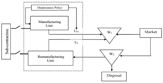
Figure 1. Closed-loop Production System.

The remanufacturing unit is also composed of one machine. The role of this remanufacturing machine is to reprocess non-disposable products returned by costumers. Like the production plan for the manufacturing machine, remanufacturing plans have to consider the quantity of emitted carbon and the penalty to be paid after exceeding a fixed level. Differently to the maintenance strategy of manufacturing unit, the preventive maintenance plan for the remanufacturing unit can be either fixed or established by choosing the number of preventive interventions because the machine has less pressure than the manufacturing unit. Time for a preventive action for the remanufacturing unit is not negligible and it is denoted by t_p.

The role of the subcontractor is to help either the manufacturing or the remanufacturing unit in order to reduce the total quantity of emitted carbon during the reprocess or the production process.

In this study, firstly, economical production plans for manufacturing, remanufacturing as well as for subcontracting units are determined. Secondly, an optimal maintenance plan is described, which is characterized by the optimal number of preventive maintenance actions for manufacturing a unit, and minimizing the total cost of production, inventory, carbon penalty and maintenance.

3. Problem Formulation

In order to establish the production plan for the finite horizon H·∆t, we will consider a quadratic cost-function based on the HMMS (Holt, Modigliani, Muth, Simon) model of [24]. This cost-function will consider production, remanufacturing, subcontracting and holding costs. Unlike the negligible maintenance time compared to manufacturing time, the preventive maintenance duration for the remanufacturing unit t_p follows a uniform distribution of parameters a and b. As shown in Figure 2, time needed for the preventive actions which take place each h.T_r is not negligible. In this study, the interval between two preventive maintenance actions for the remanufacturing unit is equal to x × ∆_t with x = {1, 2, …, H}. In what follows, time for preventive actions t_p will be expressed by t_p = y × ∆_t with y follows a uniform distribution of parameters a and b. In this case, the maintenance of the remanufacturing machine begins and ends in the same production period k.

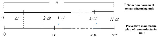
Figure 2. Production and preventive maintenance horizon.

3.1. Production Policy

Our objective is to establish an economic production by considering the constraint of the amount of carbon allowed to be emitted during the process. In order to do that and determine the economic lots to be produced each period, we will proceed by minimizing the total cost-function composed of manufacturing, remanufacturing, subcontracting, holding and costs of exceeding the allowed amount of carbon.

3.1.1. Carbon Emission Quantity

During remanufacturing and manufacturing process, a certain quantity of carbon, proportional to the lot-sizes, is emitted. In order to reduce greenhouse gas emission, the government imposed a maximal amount of carbon emission denoted by Q_cm(0) for the manufacturing unit and Q_cr(0) for the remanufacturing unit. After exceeding this amount, companies will have to pay a penalty depending on the quantity emitted. So the remaining quantity of carbon after the emitting in each period by manufacturing and remanufacturing unit will be expressed by:

$$Q_m\left(k\right)=Q_{cm}\left(0\right)-{\displaystyle \sum }_{j=1}^k{P}_m\left(j\right)\times {\Delta }_t\times \xi$$

(1)

$$Q_r\left(k\right)=Q_{cr}\left(0\right)-{\displaystyle \sum }_{j=1}^k{P}_r\left(j\right)\times {\Delta }_t\times \xi$$

(2)

where P_m(k) and P_r(k) are the lots produced respectively by manufacturing and remanufacturing units in the period k.

3.1.2. Production Rates

●  Manufacturing unit

For the manufacturing unit, the production quantity can vary from period to another, which depends on the random demand and the inventory. Furthermore, since the time of maintenance is negligible compared to production time, the production rate denoted by P_m(k) can vary from the minimal production rate P_mmin to the maximal production rate of the machine P_mMAX.

●  Remanufacturing unit

Concerning the remanufacturing unit, the quantity of remanufacturing unit depends on the inventory level corresponding to products returned by customers. Unlike the case of manufacturing unit, the remanufacturing unit may not produce the total duration of the period if its production period overlaps the preventive maintenance period. In this case the preventive maintenance and production periods intersects in only one period. To identify this period, we introduce a binary variable b_k which takes 1 if the production period will overlap with a preventive action and 0 if else.

$$b_k=\{\begin{array}{c}1 \\ 0\end{array}\begin{array}{c}if k=\lfloor h\times x\rfloor \forall h\in \{1,\dots ,\lfloor \frac{H}{x}\rfloor \}\\ else\end{array}$$

The quantity to be reprocessed each period by the remanufacturing unit is represented as follows:

$$P_r\left(k\right)=\left(1-b_k\right)\times P_r\left(k\right)+b_k\times \left(1-y\right)\times P_r\left(k\right)$$

(3)

with P_r(k) the quantity reprocessed when the production and preventive action does not overlap. Under these condition P_r(k) can vary from P_rmin to P_rMAX.

● Subcontractor Unit

In order to reduce the quantity of the emitted carbon by the manufacturing and remanufacturing unit, the firm can call on a subcontractor unit. In this work, this unit can only help either in the production or the reprocess of the returned products. For this, we introduce the binary variable α_k which takes 1 if subcontractor unit will help in the manufacturing. The expression of lots produced by subcontractor unit will be expressed as follows:

$$P_s\left(k\right)={\alpha }_k\times P_s\left(k\right)+\left(1-{\alpha }_k\right)\times P_s\left(k\right)$$

(4)

The question that may arise here is: under what condition will the subcontractor assist in manufacturing, not in remanufacturing? To set this condition, we will define two functions by interval depending on the amount of emitted carbon by manufacturing and remanufacturing units. We will assign a number from 1 to 4 to four different zones proportional to the quantity of emitted carbon. These functions will be expressed as follows:

$$f_m\left(Q_m\right)=\{\begin{array}{c}1 if Q_{1m}\le Q_m\le Q_{mMAX}\\ 2 if Q_{2m}\le Q_m\le Q_{1m}\\ 3 if 0\le Q_m\le Q_{2m}\\ 4 if Q_m\le 0\end{array}$$

$$f_r\left(Q_r\right)=\{\begin{array}{c}1 if Q_{1r}\le Q_r\le Q_{rMAX}\\ 2 if Q_{2r}\le Q_r\le Q_{1r}\\ 3 if 0\le Q_r\le Q_{2r}\\ 4 if Q_r\le 0\end{array}$$

The quantities of carbon defining intervals (Q_1m, Q_2m, Q_2r, …) are set by the firm depending on the maximal amount permitted by government (Figure 3). If f_m < f_r means that remanufacturing unit is closer to the maximum allowed quantity, the subcontractor will then assist the remanufacturing unit in the reprocess of returned products. Since the pressing of the manufacturing machine is more compared to the remanufacturing unit, we also assume that assistance of manufacturing unit has priority. This means that if f_m = f_r subcontractor unit will assist manufacturing unit. Under these assumptions, the function ensuring the switching of subcontractor from a unit to another is:

$${\alpha }_k=\{\begin{array}{c}1 if f_m\ge f_r \\ 0 else\end{array}$$

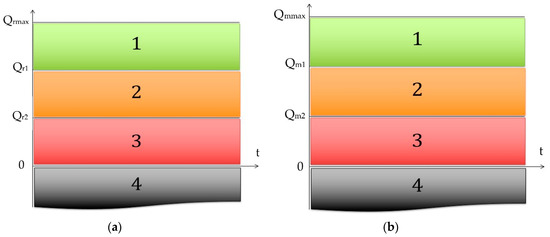
Figure 3. Dashboard functions. (a) Remanufacturing Unit; (b) Manufacturing Unit.

3.1.3. Inventory Level

Our system is composed of two warehouses. The first one has the role of stocking finite products after reprocess and production process. The second established to stock products returned by costumers denoted by β after a fixed period ρ. After disposing of ${\varphi }_k$ of the returned products that cannot be reprocessed, the remanufacturing treats the defective product to be stocked in the first warehouse. The inventory level of these warehouses is denoted by $w_m\left(k\right)$ for the first warehouse and $w_r\left(k\right)$ for the second one. $w_m\left(k\right)$ and $w_r\left(k\right)$ are computed at the end of each period and they are expressed by:

$$\begin{array}{ll}{w}_m\left(k+1\right)& =w_m\left(k\right)+\left[P_m\left(k\right)+{\alpha }_k\times P_s\left(k\right)\right]\\ & +\left[\left(\left(1-b_k\right)\times P_r\left(k\right)+b_k\times \left(1-y\right)\times P_r\left(k\right)\right)+\left(1-{\alpha }_k\right)\times P_s\left(k\right)\right]-D\left(k\right)\end{array}$$

(5)

$$w_m\left(k+1\right)=w_m\left(k\right)+P_{MT}\left(k\right)+P_{RT}\left(k\right)-D\left(k\right)$$

$$\begin{array}{ll}{w}_r\left(k+1\right)& =w_r\left(k\right)+\beta \times D\left(k-\rho \right)\times \left(1-{\varphi }_k\right)\\ & -\left[\left(\left(1-b_k\right)\times P_r\left(k\right)+b_k\times \left(1-y\right)\times P_r\left(k\right)\right)+\left(1-{\alpha }_k\right)\times P_s\left(k\right)\right]\end{array}$$

$$w_r\left(k+1\right)=w_r\left(k\right)+\beta \times D\left(k-\raisebox{1ex}{$\rho $}\!\left/ \!\raisebox{-1ex}{$\Delta t$}\right.\right)\times \left(1-{\varphi }_k\right)-P_{RT}\left(k\right)$$

(6)

where:

$$P_{MT}\left(k\right)=\left[P_m\left(k\right)+{\alpha }_k\times P_s\left(k\right)\right]$$

$$P_{RT}\left(k\right)=\left[\left(\left(1-b_k\right)\times P_r\left(k\right)+b_k\times \left(1-y\right)\times P_r\left(k\right)\right)+\left(1-{\alpha }_k\right)\times P_s\left(k\right)\right]$$

3.1.4. Service Level

In order to prevent the shortage of stock and ensure the continuity of the service even when there is unexpected variation in the demand from period to another, we impose the probabilistic condition where the probability of a positive inventory level corresponding to the finished products is greater than θ (where θ ∈ [0,1]).

$$P\left[w_m\left(k+1\right)\ge 0\right]\ge \theta$$

(7)

3.1.5. Subcontractor Solution

To allocate the quantities to be produced or reprocessed by the principal manufacturing machine, the remanufacturing or subcontractor units, we will introduce γ which follows a uniform distribution of parameters p₁ = 0 and p₂ = 0.5. So that:

$$P_{MT}\left(k\right)=P_m\left(k\right)+{\alpha }_k\times P_s\left(k\right)=\gamma \times P_{MT}\left(k\right)+\left(1-\gamma \right)\times P_{MT}\left(k\right)$$

(8)

$$P_{RT}\left(k\right)=P_r\left(k\right)+(1-{\alpha }_k)\times P_s\left(k\right)=\gamma \times P_{RT}\left(k\right)+\left(1-\gamma \right)\times P_{RT}\left(k\right)$$

(9)

with γ ∈ [p₁, p₂].

For cost optimization purpose, we will also add a binary variable τ which takes 1 if the cost of penalty due to exceeding the allowed amount of carbon is greater to the cost to be paid to the subcontractor.

$$\tau =\{\begin{array}{c}1 if C_{carbon}\ge C_{subcontractor}\\ 0 else\end{array}$$

The lots to be produced for the example of α_k = 1 will be expressed by:

$$P_{MT}\left(k\right)=P_m\left(k\right)+P_s\left(k\right)=\gamma \times P_{MT}\left(k\right)+\left(1-\gamma \right)\times P_{MT}\left(k\right)$$

With

$$P_m\left(k\right)=\tau \times \gamma \times P_{MT}\left(k\right)+\left(1-\tau \right)\times \left(1-\gamma \right)\times P_{MT}\left(k\right)$$

$$P_s\left(k\right)=\left(1-\tau \right)\times \gamma \times P_{MT}\left(k\right)+\tau \times \left(1-\gamma \right)\times P_{MT}\left(k\right)$$

• If the cost of carbon is greater than the cost of subcontracting, the manufacturing unit will produce the minimal quantity $\gamma \times P_{MT}\left(k\right)$ and the subcontractor unit will produce the remaining $\left(1-\gamma \right)\times P_{MT}\left(k\right)$.
• If the cost of subcontracting is greater than the cost of carbon (τ = 0), then minimal quantity will be produced by the subcontractor unit.

3.1.6. Cost Functions

We recall that our objective is to elaborate an optimal production plan for a finite horizon H·∆_t. We have processed by minimizing the total cost-function composed of inventory holding, production and the penalty for exceeding the allowed amount.

$$C_T={\displaystyle \sum }_{k=1}^{H-1}\left[C_{hold}\left(k\right)+C_{prod}\left(k\right)+C_{carbon}\left(k\right)\right]+C_{hold}\left(H\right)$$

(10)

Carbon penalty:

In order to restrict the amount of emitted carbon by factories during its activities, the government imposes a penalty to be paid after exceeding the allowed quantity:

$$C_{carbon}\left(k\right)=C_c\times \left(\left|Q_m\left(k\right)\right|\times {\mathbf{1}}_{Q_m\left(k\right)<0}+\left|Q_r\left(k\right)\right|\times {\mathbf{1}}_{Q_r\left(k\right)<0}\right)$$

(11)

Production cost:

Based on the HMMS model of [22], production cost of manufacturing, remanufacturing and subcontractor units will be expressed by:

$$\begin{gathered} C_{prod}\left(k\right)=C_{pm}\times {\left[P_m\left(k\right)\right]}^2+C_{pr}\times {\left[P_r\left(k\right)\right]}^2+C_{ps}\times {\left[P_s\left(k\right)\right]}^2 \\ {C}_{prod}\left(k\right)=C_{pm}\times {\left[P_m\left(k\right)\right]}^2+C_{pr}\times {\left[\begin{array}{c}\left(1-b_k\right)\times P_r\left(k\right) \\ +b_k\times \left(1-y\right)\times P_r\left(k\right)\end{array}\right]}^2+C_{ps}\times {\left[P_s\left(k\right)\right]}^2 \end{gathered}$$

(12)

where $C_{pm}$, $C_{pr}$ and $C_{ps}$ are the unit cost of manufacturing, remanufacturing and subcontracting.

Inventory holding cost:

Like the production cost, inventory holding cost will be also based on the HMMS model.

$$C_{hold}\left(k\right)=C_{hm}\times E{\left[w_m\left(k\right)\right]}^2+C_{hr}\times E{\left[w_r\left(k\right)\right]}^2$$

(13)

$C_{hm}$ and $C_{hr}$ represent the cost of holding one unit of finished product and returned product.

The total cost-function will be expressed as follows:

$$\begin{array}{ll}{C}_T& =C_{hm}\times E{\left[w_m\left(H\right)\right]}^2\\ & +{\displaystyle {\displaystyle \sum }_{k=1}^{H-1}}[C_{hm}\times E{\left[w_m\left(k\right)\right]}^2+C_{pm}\times {\left[P_m\left(k\right)\right]}^2\\ & +C_c\times (|Q_m\left(k\right))|\times {\mathbf{1}}_{Q_m\left(k\right)<0}]+C_{hr}\times E{\left[w_r\left(H\right)\right]}^2\\ & +{\displaystyle {\displaystyle \sum }_{k=1}^{H-1}}[C_{hr}\times E{\left[w_r\left(k\right)\right]}^2+C_{pr}\times {\left[P_r\left(k\right)\right]}^2+C_c\times (|Q_r\left(k\right))|\times {\mathbf{1}}_{Q_r\left(k\right)<0}]\\ & +{\displaystyle {\displaystyle \sum }_{k=1}^{H-1}}{C}_{ps}\times {\left[P_S\left(k\right)\right]}^2\end{array}$$

(14)

3.2. Maintenance Strategy

In this section, we propose an optimal maintenance strategy for the manufacturing unit according to the production plan obtained by the production policy. The maintenance strategy is characterized by a preventive maintenance strategy with minimal repair. The preventive maintenance activities are performed periodically during the finite horizon of production H·∆t. In this case, the finite production horizon is divided equally into N intervals T ($T=a\times {\Delta }_t$) of maintenance with N·T = H·∆t. A perfect preventive maintenance action is performed at each time $q\times T,q=1,\dots ,N$ to restore the manufacturing unit to as good as new state. A minimal repair (as bad as old) is performed when there a failure between two preventive maintenance actions without changing the state of failure rate of the manufacturing unit.

The objective of this strategy is to determine the optimal number of preventive maintenance actions N for the manufacturing unit by minimizing the total maintenance cost.

The total cost of maintenance is followed by the equation:

$$C_M\left(N\right)=M_p\cdot \left(N-1\right)+M_c\cdot \phi \left(N\right)$$

(15)

with $\phi \left(N\right)$: average number of failures during [0, H·∆t] for manufacturing unit.

The average number of failure is calculated according to the function of failure rate. On the other hand, failure rate is influenced by the variation of the production cadence and given by the following cumulative function:

$${\lambda }_k\left(t\right)={\lambda }_{k-1}\left(\Delta t\right)+\frac{P_m(k)}{P_{mMax}} {\lambda }_n\left(t\right)$$

(16)

with ${\lambda }_n\left(t\right)$ presenting the nominal failure rate for the manufacturing unit when the unit worked with its maximal production rate during the all finite horizon H·∆t (Figure 4).

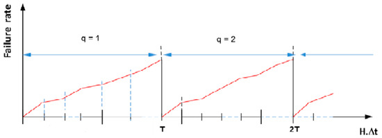
Figure 4. Failure rate evolution.

The average number of failure for manufacturing unit presented as:

$$\phi \left(N\right)={\displaystyle \sum }_{i=0}^{\lfloor \frac{H\cdot \Delta t}{T}\rfloor -1}\left[{\displaystyle \sum }_{k=In\left(i+\frac{T}{\Delta t}\right)+1}^{In\left(\left(i+1\right)\times \frac{T}{\Delta t}\right)}\underset{0}{\overset{\Delta t}{{\displaystyle \int }}}{\lambda }_k\left(t\right)dt\right]+{\displaystyle \sum }_{k=\lfloor \frac{H\cdot \Delta t}{T}\rfloor \times \frac{T}{\Delta t}}^H\underset{0}{\overset{\Delta t}{{\displaystyle \int }}}{\lambda }_k(t)dt$$

(17)

with N = H·∆t/T.

4. Optimization Approach

Our objective is to find the optimal lot-sizes to be produced by the manufacturing, remanufacturing and subcontractor units P_M, P_R and P_s and the optimal number of preventive maintenance actions for the manufacturing unit minimizing the total cost-function of production, inventory and maintenance.

Due to the stochastic nature of our problem, it would be difficult to find an optimal solution. It is therefore preferable to transform our model into a deterministic problem in order to facilitate its resolution. To do this, we use the “equivalent-certain” approach which consists of associating the variables with their average values and considering that the variation of the random demand follows a law Gaussian distribution [25] and [26]. The demand being a random variable, it affects the stock level value w_m(k) which becomes a stochastic variable while the production rates are deterministic variables.

The proof of different transformation is made in Appendix A.

The steps of the resolution method are given by the following algorithm:

-

Step 1: Generate randomly a first solution for production plan: vector of production rates of manufacturing and remanufacturing units;

-

Step 2: Check if the service level constraint is verified for the current solution;

-

Step 3: Compute the amount of emitted carbon from the manufacturing and remanufacturing units;

-

Step 4: Determine in which zone are both the manufacturing and remanufacturing units:

• Step 4.1: If the quantity of carbon of the manufacturing unit is greater to the quantity of carbon of the remanufacturing unit, we compare the cost of carbon to the cost of subcontractor:

  -

  If the cost of carbon is greater than the cost of subcontracting, then, the manufacturing unit will produce the minimal quantity γ·P_MT(k) and the subcontractor unit will produce the remaining (1 − γ)·P_MT(k).

  -

  Else, minimal quantity will be produced by the subcontractor unit.

• Step 4.2: Else, we compare the cost of carbon to the cost of subcontractor:

  -

  If the cost of carbon is greater than the cost of subcontracting, then, the remanufacturing unit will produce the minimal quantity γ·P_MT(k) and the subcontractor unit will produce the remaining (1 − γ)·P_MT(k).

  -

  Else, minimal quantity will be produced by the subcontractor unit.

5. Numerical Example

In this numerical example, we assume that the finite production horizon equals to H = 12·Δ_t with period length Δ_t = 1. The index of service level is θ = 90%. The demand is random characterized by the means that are given in Table 1 and the standard deviation is fixed for all production periods and equals to σ_d = 100. The initial inventory level w_m(k = 0) = w_r(k = 0) = 0.

Table 1. Production plan during H = 12 periods.

Periods	Demands	Manufacturing	Remanufacturing	αk	Subcontractor	wm	wr
1	1961	1491	0	1	639	169	0
2	1833	1579	0	1	677	593	0
3	1975	1496	101	1	374	589	683
4	1984	1861	54	0	15	584	565
5	2024	1725	11	0	103	399	846
6	2049	1834	19	0	32	235	795
7	2081	1376	120	1	590	240	1080
8	1962	1258	137	1	839	512	942
9	2048	1551	137	1	665	817	1013
10	1775	588	96	1	1372	1097	1898
11	1909	357	78	1	1430	1076	2208
12	2042	371	123	1	1485	1013	2617

-

Lower and upper boundaries of manufacturing and remanufacturing capacities: P_mmin = 1500; P_mMax = 2300; P_rmin = 50; P_rMax = 150;

-

Assuming the degradation law of the manufacturing unit is characterized by the Weibull distribution with two parameters shape η = 2 and scale β = 100.

The other data of the problem are presented as following

• Cost coefficients: C_hm = 20; C_hr = 25; C_pm = 30; C_pr = 25; C_ps = 35; C_c = 1250;
• Carbon coefficients: ξ = 9.3; Q_cm = 118,000; Q_cr = 2000; Q_1m = 0.6 × Q_cm; Q_2m = 0.4 × Q_cm; Q_1r = 0.8 × Q_cr; Q_2r = 0.4 × Q_cr; ρ = 2;

For the maintenance strategy, the failure rate of manufacturing unit follows the Weibull distribution with factors shape γ = 2 and scale β = 100 and the unit costs of preventive and corrective maintenance actions are respectively M_p = 500 and M_c = 2000.

5.1. Production Results

5.2. Interpretations

We can remark from Table 2 that the remanufacturing has exceeded the allowed amount of emitted carbon (negative value of the amount of carbon Q_r without subcontracting). This means that the remanufacturing unit is in the fourth zone of our indicator function defined earlier while the manufacturing unit is still in the third zone. The subcontractor unit will then assist the remanufacturing unit in Periods 4, 5 and 6 in order to reduce the emitted quantity of carbon.

Table 2. Amount of emitted carbon during the different process.

Period	1	2	3	4	5	6	7	8	9	10	11	12
Qm without subcontracting	98,191	77,210	59,819	42512	26,469	9413	−8871	−28,373	−48,972	−67,200	−83,819	−101,080
Qm	104,134	89,449	75,536	58229	42,186	25130	12,333	634	−13790	−19259	−22,579	−26,029
Qr without subcontracting	2000	2000	1061	−334	−1395	−1887	−3003	−4352	−5626	−6519	−7737	−8881
Qr	2000	2000	1061	559	456	280	−837	−2111	−3385	−4278	−5003	−6147

Using this optimization method, the amount of emitted carbon by both manufacturing and remanufacturing units is reduced. In fact, we can remark from Figure 5 and Table 2 that we succeeded in delaying exceeding the allowed amount from the 7th Period to the 9th Period for the manufacturing unit and from the 4th Period to the 7th Period for the remanufacturing unit. Additionally, this method allows us to reduce the emission of carbon even after exceeding the allowed amount. We were able to save 75,051 mu for the manufacturing unit and 2734 mu for the remanufacturing unit.

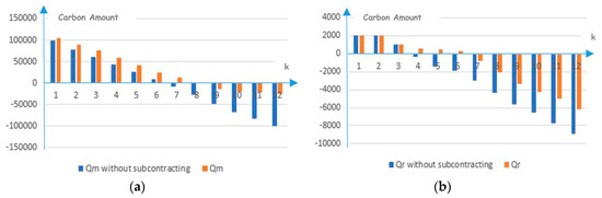
Figure 5. Amount of emitted carbon with and without subcontracting unit. (a) Manufacturing unit; (b) Remanufacturing unit.

For optimization purpose, if the cost of subcontracting is greater than the cost of carbon, the maximal lot-sizes will be affected to the manufacturing or the remanufacturing units. We can remark by analyzing the Table 3 that this condition is satisfied. For the first three periods, the subcontractor will assist in the remanufacturing by taking the minimal lot size because the cost of carbon is null (this unit did not exceed the allowed amount). For the three next periods, the subcontractor will assist in the remanufacturing in the fourth period, the subcontractor will take the smaller lot size because the cost of subcontracting is greater than the penalty of exceeding the allowed amount. In the 5th and 6th Periods, the penalty cost will exceed the cost of subcontracting, which is why the remanufacturing will take the minimal lot size. This is the same case for the three last periods where the subcontractor unit will assist in the manufacturing and takes the maximal lot size.

Table 3. Production plan with C_ps = 35; C_c = 3550.

Period	Lot Produced by Manufacturing Unit	Lot Produced by Remanufacturing Unit	αk	Lot Produced by Subcontracting Unit	wm	wr
1	1563	0	1	670	271	0
2	1754	0	1	438	435	0
3	1713	87	1	428	768	894
4	1751	47	0	13	597	1805
5	2252	11	0	97	964	1887
6	1988	17	0	53	909	1816
7	825	119	1	1237	1120	1697
8	349	97	1	1398	782	1599
9	324	118	1	1294	436	1875
10	187	55	1	1685	234	2256
11	211	67	1	1895	310	2796
12	799	54	1	1199	291	2742

5.3. Maintenance Results

From Figure 6, the ideal number of preventive maintenance activities for manufacturing unit N = 4 with an optimum interval between two perfect PM T* = 3·Δt. In this case, we can conclude that the principal production unit produces more compared to the remanufacturing unit and consequently the failure rate of the manufacturing unit grows faster, as does the optimum number of preventive maintenance activities.

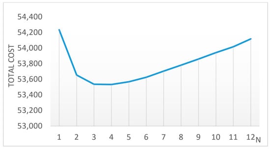
Figure 6. Optimal number of preventive maintenance actions.

5.4. Sensitivity Study

5.4.1. Impact of Costs Variability

- C_ps = 35 and C_c = 3550

From Figure 7 and Figure 8 and Table 3 and Table 4, the bigger gap between the subcontractor unit cost and the cost of carbon penalty, the longer the subcontractor unit will take to produce and the larger the amount of carbon emitted during the production process. This result is predictable because the of the firm aim to minimize its total cost-function, which means that if the cost of penalty is bigger than the cost of subcontracting, the firm will try to minimize the emission of carbon in order to minimize the total cost.

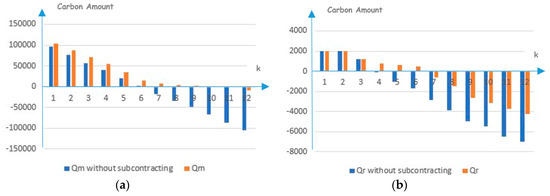
Figure 7. Amount of emitted carbon with and without subcontracting unit for C_ps = 35; C_c = 3550. (a) Manufacturing unit; (b) Remanufacturing unit.

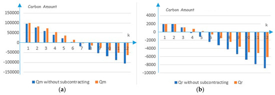
Figure 8. Amount of emitted carbon with and without subcontracting unit for C_ps = 500; C_c = 550. (a) Manufacturing unit; (b) Remanufacturing unit.

Table 4. Production plan with C_ps = 500; C_c = 550.

Period	Lot Produced by Manufacturing Unit	Lot Produced by Remanufacturing Unit	αk	Lot Produced by Subcontracting Unit	wm	wr
1	1600	0	1	686	391	0
2	1160	0	1	774	253	0
3	1172	100	1	781	215	279
4	2083	84	0	27	458	786
5	2274	30	0	46	798	710
6	1838	48	0	48	773	606
7	1151	106	1	768	819	1103
8	1456	58	1	364	755	2026
9	1197	54	1	798	896	2368
10	1768	71	1	196	889	2491
11	1798	52	1	200	845	2427
12	1287	89	1	551	830	2951

- C_ps = 500 and C_c = 550

We can also remark that the gap between the quantity of emitted carbon during the remanufacturing process with and without subcontracting remains almost the same in the final period (around 2000 mu). This is mainly due to the priority order (the manufacturing unit has priority). In fact, the subcontractor will not take the maximal lot until one of our units has exceeded its allowed amount (which means that the indicator function corresponding to this unit will take 4). If both manufacturing and remanufacturing units exceed respectively Q_cm and Q_rm, then the subcontractor will assist in the manufacturing. Which is why we remark in our case that the gap between Q_r with and without subcontracting remains almost the same in the final period when both units have exceeded their allowed amount.

5.4.2. Impact of the Variability of the Proportion of emitted Carbon

From Table 5 and Table 6, we can remark that the variability of the proportion of emitted carbon to produce an item has an impact on the decision variable α_k which indicates whether the subcontractor assists in the manufacturing or in the remanufacturing. In fact, by increasing the proportion of emitted carbon while maintaining the maximal allowed amount constant, both units will exceed this quantity earlier, which means that their indicator functions will take 4 and due to the priority order the subcontractor will assist in the manufacturing. By decreasing the value of ξ, the remanufacturing unit will exceed its allowed amount earlier than the manufacturing unit because Q_cm is greater than Q_rm. The indicator function of the remanufacturing is likely to take a bigger value than the one corresponding to the manufacturing unit. This means that the subcontractor unit will help the manufacturing unit in order to reduce its emission of carbon.

Table 5. Amount of emitted carbon during the different process with ξ = 6.3.

Period	1	2	3	4	5	6	7	8	9	10	11	12
αk	1	1	0	0	0	0	0	0	1	1	1	1
Qm without subcontracting	104,178	91,068	77,630	65,464	51,604	38,475	25,522	13,666	−484	−12,240	−26,390	−39,305
Qm	109,709	101,841	88,403	76,237	62377	49,248	36,295	24,439	14,535	3957	−5946	−11,112
Qr without subcontracting	2000	2000	1345	526	−350	−841	−1465	−2057	−2719	−3172	−3689	−4199
Qr	2000	2000	1540	923	835	797	734	520	−142	−596	−715	−1226

Table 6. Amount of emitted carbon during the different process with ξ = 15.8.

Period	1	2	3	4	5	6	7	8	9	10	11	12
αk	1	1	0	1	1	1	1	1	1	1	1	1
Qm without subcontracting	81,723	45,984	18,586	−10,501	−39,889	−68,819	−103,216	−134,042	−166,274	−202,234	−232,839	−264,297
Qm	96,228	71,216	43,819	17,638	11,761	3087	−358	−6520	−16,189	−26,981	−36,161	−48737
Qr without subcontracting	2000	2000	−101	−2471	−4146	−6279	−7496	−8444	−10,672	−12,520	−14,179	−16,407
Qr	2000	2000	531	-449	−2124	−3862	−5078	−5868	−8096	−9945	−11,272	−13,500

5.4.3. Impact of the Variability of the Allowed Amount of Carbon

To better appreciate the sensibility of our model to the variability of the allowed amount of carbon, we fixed the cost of carbon C_c = 2250 and the cost of subcontracting C_ps = 35.

We can remark that by reducing the allowed amount of one unit while maintaining the other constant like the case of Table 7 and Table 8, the number of interventions of the subcontractor unit to help this unit will increase, because when WC decreases the concerned unit will deplete this quantity earlier and the subcontractor will have to help to reduce the emission of carbon. We can reason in the same way when we increase the allowed amount like the case of Table 9 and Table 10. The number of interventions of the subcontractor unit to help this unit this time will decrease. If Q_cr increase and Q_cm remains constant, the remanufacturing unit will deplete its allowed amount later. The subcontractor will assist then more in the manufacturing. The same case when Q_cm increase and Q_cr remains constant, the manufacturing unit will deplete its allowed amount later and the subcontractor will assist then more in the remanufacturing.

Table 7. Amount of emitted carbon during the different process with Q_cm = 200,000 and Q_cr = 2000.

Period	1	2	3	4	5	6	7	8	9	10	11	12
αk	1	1	1	0	0	0	0	0	0	0	0	0
Qm without subcontracting	235,586	222,129	208,590	194,623	180,637	170,746	160,861	146,529	134,697	120,617	108,011	96,545
Qm	238,471	227,704	219,584	205,617	191,631	181,740	171,855	157,522	145,691	131,610	119,004	107,538
Qr without subcontracting	2000	2000	1654	1105	438	−38	−822	−1635	−2026	−2706	−3286	−3985
Qr	2000	2000	1654	1471	1068	929	816	595	475	274	186	116

Table 8. Amount of emitted carbon during the different process with Q_cm = 50,000 and Q_cr = 2000.

Period	1	2	3	4	5	6	7	8	9	10	11	12
αk	1	1	1	1	1	1	1	1	1	1	1	1
Qm without subcontracting	29670	9443	−9929	−30,547	−45,939	−61,414	−80,721	−95,210	−112,797	−129,583	−150,629	−167,741
Qm	35,771	23,635	12,010	3760	−2396	−5493	−9353	−10,803	−12,561	−14,244	−18,457	−21,880
Qr without subcontracting	2000	2000	1163	605	−176	−651	−2036	−3422	−4752	−5998	−7337	−8667
Qr	2000	2000	1163	735	−46	−455	−1841	−3134	−4464	−5710	−6203	−7533

Table 9. Amount of emitted carbon during the different process with Q_cm = 118,000 and Q_cr = 1500.

Period	1	2	3	4	5	6	7	8	9	10	11	12
αk	1	1	0	0	0	0	1	1	1	1	1	1
Qm without subcontracting	97,903	78,615	58,685	40,475	22,461	4493	−13,939	−32,995	−52,767	−69,972	−88,702	−106,688
Qm	105,938	92,434	72,504	54,295	36,281	18,313	3563	−13,586	−31,377	−36,538	−40,286	−43,885
Qr without subcontracting	1500	1500	468	−295	−1671	−2211	−3355	−3996	−4657	−5326	−5847	−6489
Qr	1500	1500	775	570	431	328	−816	−1337	−1997	−2666	−3104	−3745

Table 10. Amount of emitted carbon during the different process with Q_cm = 118,000 and Q_cr = 3500.

Period	1	2	3	4	5	6	7	8	9	10	11	12
αk	1	1	1	1	1	1	1	1	1	1	1	1
Qm without subcontracting	97,428	77,015	56,248	36,439	16,835	−2277	−20,830	−41,821	−62,913	−82,266	−98002	−114,156
Qm	101,539	85,208	72,746	58,880	41,238	27855	13,012	−5876	−10,098	−13,967	−15,539	−20,384
Qr without subcontracting	3500	3500	2356	1826	970	−229	−1615	−2936	−3856	−4870	−5335	−6246
Qr	3500	3500	2356	2012	1156	385	−1001	−2173	−3094	−4107	−4405	−5316

The approach proposes a new joint production and maintenance policy, which considers an environmental aspect for a forecasting problem of a reverse logistic system subject to a random degradation. The satisfaction of a random demand under a given service level, and at the same time respecting the environmental constraint characterized by the harmful emissions to the environment, may be sanctioned by an environmental tax, and requires that the company has found new strategies to meet these different objectives. The objective of this study is to propose an environmental production and maintenance policy optimization by proposing the subcontractor as a solution in order to satisfy the random demand and decrease the carbon tax. In this context, an economical production plans for the manufacturing, remanufacturing and subcontract units as well as an optimal maintenance strategy by developing a correlation between the production and maintenance. Firstly, we have integrated the subcontractor solution on the production policy under a new switching approach which determines when the subcontractor can help either manufacturing or remanufacturing a unit during the production according to the dashboard, which defines different sectors of the quantity of emitted carbon in order to minimize the total cost of production, inventory and carbon tax. Secondly, using a sequential approach by integrating the economical production plan of manufacturing unit obtained by the production policy in the maintenance strategy, we determine the optimal number of preventive maintenance actions. The originality of this study in maintenance terms is to consider the influence of the production variation on the degradation degree of the manufacturing unit by establishing a correlation between the production and maintenance characterized by an analytical equation that shows the failure rate progress of the manufacturing unit according to its use, respecting at the same time the continuity of the reliability of the manufacturing unit from one period to another.

6. Conclusions

In this study, we have proposed an integrated maintenance-to-production model for a reverse logistic system in order to minimize the total cost of production, inventory, Carbon tax and maintenance. A subcontractor is integrated in the model as a solution to minimize the quantity of emitted carbon and its tax by the manufacturing and remanufacturing. The proposed idea is to consider a dashboard of management to develop a condition for the intervention of subcontractor to help the manufacturing or remanufacturing units. To resolve this problem, firstly, a production policy is developed in order to determine the economic plan of production for the manufacturing and remanufacturing units as well as the plan of the switching subcontractor intervention. Secondly, by considering the impact of the failure rate of manufacturing unit by the variation of production cadences, we propose an optimal preventive maintenance strategy block type under economic criteria to obtain the best amount of preventive maintenance applied during the finite horizon.

For further research, we could consider the impact of the quality (bad, average, high) of the returned products by the customer on the degradation of the remanufacturing unit as well as its quantity of emission.

References

- Barreto, L.; Kypreos, S. Emissions trading and technology deployment in an energy-systems “bottom-up” model with technology learning. Eur. J. Oper. Res. 2004, 158, 243–261. [Google Scholar] [CrossRef]
- Martin, R.; Preux, L.B.; Wagner, U.J. The Impact of a Carbon Tax on Manufacturing: Evidence from Microdata. J. Public Econ. 2014, 117, 1–14. [Google Scholar] [CrossRef]
- Allevi, E.; Gnudi, A.; Konnov, I.V.; Oggioni, G. Evaluating the effects of environmental regulations on a closed-loop supply chain network: A variational inequality approach. Ann. Oper. Res. 2018, 1, 1–43. [Google Scholar] [CrossRef]
- Hua, G.; Cheng, T.C.E.; Wang, S. Managing Carbon Footprints in Inventory Management. Int. J. Prod. Econ. 2011, 132, 178–185. [Google Scholar] [CrossRef]
- Yuan, B.; Gu, B.; Guo, J.; Xia, L.; Xu, C. The Optimal Decisions for a Sustainable Supply Chain with Carbon Information Asymmetry under Cap-and-Trade. Sustainability 2018, 10, 1002. [Google Scholar] [CrossRef]
- Sambodo, M.T. Investigating the impact of carbon tax to power generation in java-bali system by applying optimization technique. In WorkinP Papers in Economics and Development Studies (WoPEDS); Department of Economics, Padjadjaran University: Jawa Barat, Indonesia, 2010. [Google Scholar]
- Parag, Y.; Capstick, S.; Poortinga, W. Policy attribute framing: A comparison between three policy instruments for personal emissions reduction. J. Policy Anal. Manag. 2011, 30, 889–905. [Google Scholar] [CrossRef]
- Böhringer, C.; Carbone, J.C.; Rutherford, T.F. Unilateral climate policy design: Efficiency and equity implications of alternative instruments to reduce carbon leakage. Energy Econ. 2012, 34, 208–217. [Google Scholar] [CrossRef]
- Matsui, K. Cost-based Transfer Pricing under R&D Risk Aversion in an lntegrated Supply Chain. Int. J. Prod. Econ. 2011, 139, 69–79. [Google Scholar]
- Toptal, A.; Çetinkaya, B. How Supply Chain Coordination Affects the Environment: A Carbon Footprint Perspective. Ann. Oper. Res. 2017, 250, 487–519. [Google Scholar] [CrossRef]
- Soleimani, F.; Khamseh, A.A.; Naderi, B. Optimal Decisions in a Dual-Channel Supply Chain under Simultaneous Demand and Production Cost Disruptions. Ann. Oper. Res. 2016, 243, 301–321. [Google Scholar] [CrossRef]
- Hajej, Z.; Dellagi, S.; Rezg, N. Joint optimisation of maintenance and production policies with subcontracting and product returns. J. Intell. Manuf. 2012. [Google Scholar] [CrossRef]
- Tang, S.; Wang, W.; Yan, H.; Hao, G. Low carbon logistics: Reducing shipment frequency to cut carbon emissions. Int. J. Prod. Econ. 2015, 164, 339–350. [Google Scholar] [CrossRef]
- Dobos, I. Tradable Emission Permits and Production-inventory Strategies of the Firm. Int. J. Prod. Econ. 2007, 108, 329–333. [Google Scholar] [CrossRef]
- Dobos, I. Production strategies under environmental constraints in an Arrow-Karlin model. Int. J. Prod. Econ. 1999, 59, 337–340. [Google Scholar] [CrossRef]
- Dobos, I. Production strategies under environmental constraints: Continuous-time model with concave costs. Int. J. Prod. Econ. 2001, 71, 323–330. [Google Scholar] [CrossRef]
- Li, S. Optimal control of production-maintenance system with deteriorating items, emission tax and pollution R&D investment. Int. J. Prod. Res. 2014, 52, 1787–1807. [Google Scholar] [CrossRef]
- Ayed, S.; Dellagi, S.; Rezg, N. Joint optimisation of maintenance and production policies considering random demand and variable production rate. Int. J. Prod. Res. 2012, 50, 6870–6885. [Google Scholar] [CrossRef]
- Hajej, Z.; Rezg, N.; Gharbi, A. Forecasting and Maintenance Problem under Subcontracting Constraint with Transportation Delay. Int. J. Prod. Res. 2014. [Google Scholar] [CrossRef]
- Dellagi, S.; Rezg, N.; Xie, U. Preventive maintenance of manufacturing systems under environmental constraints. Int. J. Prod. Res. 2007, 45, 1233–1254. [Google Scholar] [CrossRef]
- Dahane, M.; Clementz, C.; Rezg, N. Effects of extension of subcontracting on a production system in a joint maintenance and production context. Compt. Ind. Eng. 2010, 58, 88–96. [Google Scholar] [CrossRef]
- Selcuk, S. Predictive maintenance, its implementation and latest trends. Proc. Inst. Mech. Eng. Part B J. Eng. Manuf. 2016, 231, 1670–1679. [Google Scholar] [CrossRef]
- Renna, P. Influence of maintenance policies on multi-stage manufacturing systems in dynamic conditions. Int. J. Prod. Res. 2012, 50, 345–357. [Google Scholar] [CrossRef]
- Holt, C.C.; Modigliani, F.; Muth, J.F.; Simon, H.A. Planning Production, Inventory and Work Force; Prentice-Hall: Englewood Cliffs, NJ, USA, 1960. [Google Scholar]
- Silva Filho, O.S.; Ventura, S.D. Optimal feedback control scheme helping managers to adjust aggregate industrial resources. Control Eng. Pract. 1999, 7, 555–563. [Google Scholar] [CrossRef]
- Silva Filho, O. Linear quadratic gaussian probelm with constraints applied to aggregated production planning. In Proceedings of the 2001 American Control Conference, (Cat. No.01CH37148), Arlington, VA, USA, 25–27 June 2001. [Google Scholar]
© 2019 by the authors. Licensee MDPI, Basel, Switzerland. This article is an open access article distributed under the terms and conditions of the Creative Commons Attribution (CC BY) license (http://creativecommons.org/licenses/by/4.0/).