Article

Efficient Characterization of Macroscopic Composite Cement Mortars with Various Contents of Phase Change Material

1
Univ. Artois, IMT Lille Douai, Univ. Lille, Yncréa Hauts-de-France, EA 4515, Laboratoire de Génie Civil et géo- Environnement (LGCgE), F-62400 Béthune, France
2
University of Pau & Pays Adour/E2S UPPA, Laboratoire de Thermique, Énergétique et Procédés—IPRA, EA 1932e, 64000 Pau, France
*
Author to whom correspondence should be addressed.
Appl. Sci. 2019, 9(6), 1104; https://doi.org/10.3390/app9061104
Submission received: 13 February 2019 / Revised: 24 February 2019 / Accepted: 27 February 2019 / Published: 15 March 2019
(This article belongs to the Special Issue Advanced Applications of Phase Change Materials)

Abstract

:
The determination of both the thermal and thermodynamical properties of a composite material containing phase change material is done thanks to an inverse method, which combines experimental measurements and numerical computations. Given first an in-house experiment, which allows us to test samples at a macroscopic scale (i.e., close to the real conditions) and to set various types of thermal stresses, and secondly the simulation of the corresponding thermal behavior, relying on an accurate thermodynamical modeling and taking into account the real operating parameters (e.g., thermal contact resistances and non-symmetric heat fluxes on each side), it is possible to characterize the solid and liquid thermal conductivities and heat capacities, as well as the temperature range associated with a non-isothermal phase transition and the associated latent heat. The specificity of the present approach is to allow, in a single step, a characterization of all the involved thermo-physical parameters that are usually required in simulation tools (e.g., EnergyPlus…). Moreover, the hitherto studies dealing with repeatability and uncertainties of the enthalpy characterization are generally very scant and not encountered very often or only with qualitative assessments. This is a clear caveat, especially when considering any system design. Therefore, for the first time ever, the present paper pays a special attention to the repeatability of the identification method and studies the scedasticity of the results, that is to say the deviations of the determined enthalpy curves, not only from a qualitative point of view but also by proposing quantitative arguments. Finally, the results are very promising since the agreement between all trials is excellent, the maximum error for all parameters being lower than 4%. This is far below the current quality thresholds admitted when characterizing the enthalpy of a phase change material.

1. Introduction

Following the effective ratification of the Paris Agreement (official version is avaiable at https://unfccc.int/sites/default/files/english_paris_agreement.pdf) by an overwhelming majority, with 185 countries over 197 parties to the Convention (as the date of February 2019), it is clear that the recent trends towards economy decarbonation and energy consumption reductions shall be pursued, specifically in Europe. Among the possible avenues of research, the lowering of the impacts of the buildings sector on energy needs appears to be a promising way. Practically, many options are nowadays available and many more practical and multi-disciplinary research projects are under development. When considering only the energy requirements for the heating and cooling in residential and commercial buildings, it is already a third of the total global use and, more importantly, it should increase by approximatively 79% and 84% between 2010 and 2050 [1,2].
To overcome the use of heating and cooling devices, the use of phase change materials (PCM) has been proposed. They can authorize to benefit from free heating or cooling or to delay the thermal stress, to name but a few examples for passive applications. As a rule of thumb, the topic of PCM has greatly focused the attention of numerous groups in the past decades, with a clear increase during the last twenty years. Thus, when considering the literature, and if one goes from the most general to the more specific, a good (subjective) starting point could be found in [3,4,5,6,7,8] or in the reviews summary proposed by [9,10].
Zhu et al. [3] focused on the thermal dynamic behaviors and the energy performance of buildings with PCM. Several important aspects on the use of PCM are withdrawn. Concerning the free cooling and the passive applications (Section 2 pp. 3170–3171 & Section 5 pp. 3173–3179), it is shown that thermal comfort can be increased yet the design process is a keyfactor. Moreover, in the former case, the concept is more interesting if a large difference in temperature between day and night exists. Then, the peak load shifting applications (Section 3 pp. 3171–3173) seem to be promising. Unfortunately, the main results usually only rely on simulations or prototypes; it is consequently difficult to have a detailed view of the energy savings. Finally, let us mention the interesting summary table of the major results (Table 1, p. 3178) and the study of the relationship between the payback time and the price of energy and the price of PCMs (Figure 1 p. 3171). In another way, a very generic and interesting discussion concerning the overall properties of PCM when applied in buildings is proposed by Cabeza et al. [9]. Generally speaking, this review presents very practical informations. A useful classification of PCMs depending on their use (Tables 3 to 8) is first given. On one hand, one can distinguish the cooling ( T M < 21 C ) and comfort ( 23 < T M < 28 C ) applications, and the heating of water ( 29 < T M < 60 C ). On the other hand, some real available commercial products are given. Classification relies on the temperature range one is interested in: 61 < T M < 120 C , T M < 21 C and 22 < T M < 28 C . In the same way, a detailed analysis of the PCMs basic requirements is given. Added to this, a classification is propposed in function of their respective melting temperatures and mass and volume latent heat. It separates PCMs in four common groups: paraffins, organics, inorganics, and eutectics (see Figure 3 p. 1686). Finally, let us mention the very enlightening discussions on stability, under thermal cycling or due to corrosion and the possible interactions between the PCMs and their containers. Last but not least, practical examples of encapsulations for commercial PCMs (Table 13 p. 1693) are presented. Issues related to over-cooling and possible segregation are also treated. Similarly, in [5], the same “taxonomy” is taken to classify the various applications, although a specific attention is given to glazing and shadings and blinds (Section 5 pp. 62–63) and to HVAC (Section 6 p. 63), and in [10]. Finally, in [7], after some basic recalls about thermal energy storages and PCMs properties, various criteria are furnished in order to help in the design and for the choice of the appropriate candidate. When turning to the encapsulation techniques, one can consider [4,6] for the micro-encapsulations and [8] for the nano-encapsulations.
If one now turns to more specific reviews, the cooling applications are addressed in [11,12,13,14,15] while specific papers are available for the appliances (or active systems), such as PV [16] and solar domestic hot water systems [17,18] or heat-pumps [19,20]. The use of PCM in structures, and the associated boons and banes, can be found in [21,22,23,24,25,26,27,28], the specific topic of mortars being detailed in [29,30]. Ling and Poon [29], after some classic recalls about PCM and their incorporation processes, propose a brief survey on the various mechanical and thermal properties determination. However, only a few numerical and practical data are available, before some discussion on their stability. In [30], Rao et al. first show that, for mortars, PCMs are mainly studied in combination with cement (Figure 11, p. 104). Secondly, their global impacts are well described, with an useful summary for the micro-encapsulated PCMs in Table 4, p. 105. Then, an extended analysis of the mechanical and thermal properties is given (see Table 6, pp. 114–115). As a rule of thumb, it appears that the determination of their effective intrinsic properties is the key factor when trying to retrieve and characterize the thermal behavior of such materials. In other words, only a confident and secure characterization will permit to estimate their real boons for buildings applications. In this respect, this is the unique solution to perform reliable and realistic simulations. This issue has been tackled by many authors:
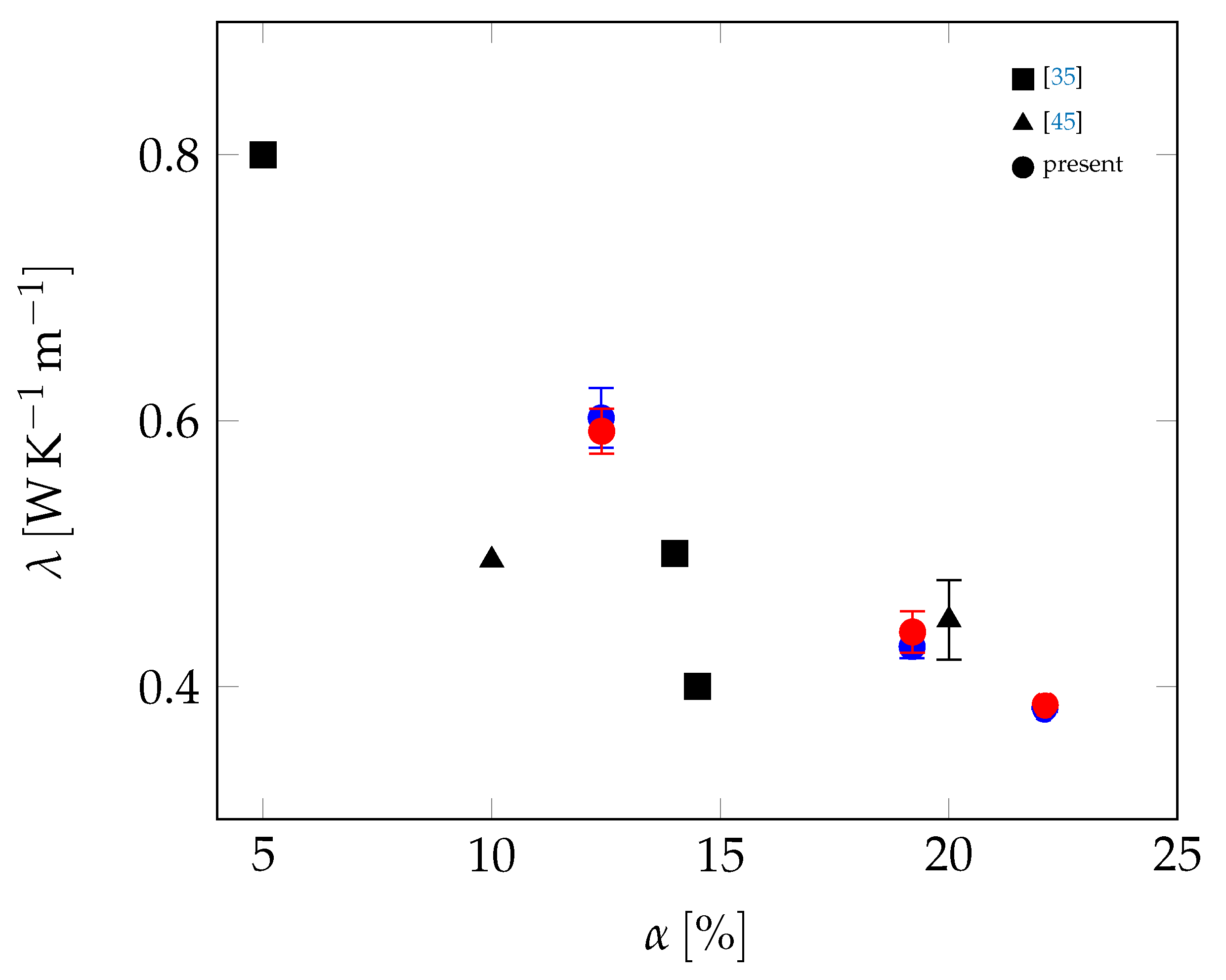
  • the thermal conductivity is searched for in [31,32,33,34,35,36,37,38,39,40,41,42,43,44,45,46] using either hot wire [31,45], hot plate [32,34,35,36,39,42,43,44,46], or laser flash [33,40] techniques.
    Let us mention here that the thermal contact resistances and their influence on the measured conductivity are rarely taken into account.
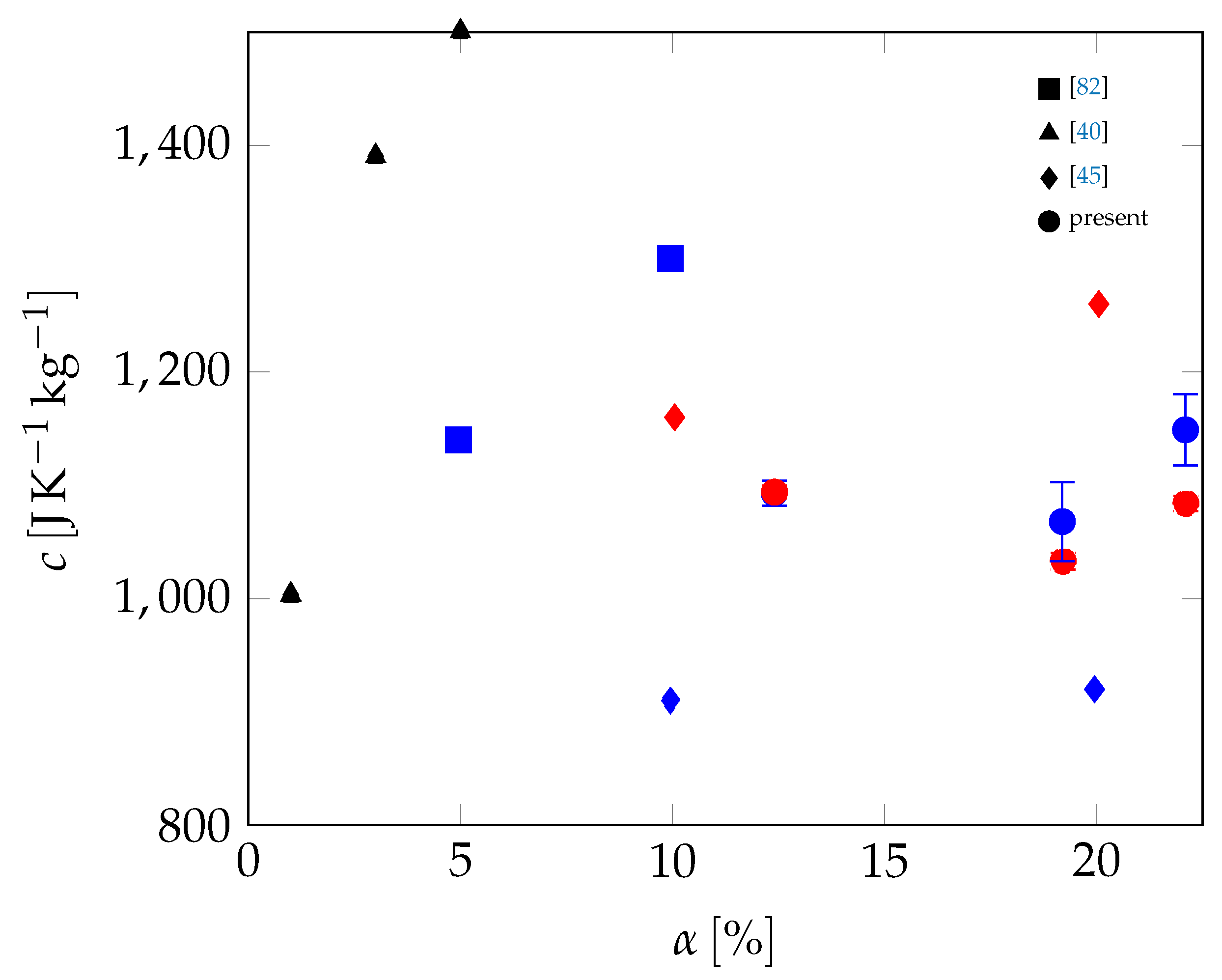
  • the heat capacity is mainly investigated as an apparent capacity, which is supposed to integrate the latent heat and goes continuously from the solid value to the liquid one [31,33,34,36,37,38,40,44,45,47,48,49,50,51,52,53]. However, many of these studies determine this property from a differential scanning calorimetry (DSC) experiment [33,34,38,40,44,45,47,48,49,50,51,53,54,55], where the size of the sample is such that it is not very representative of the macroscopic material [5,31,36,52]. As far as real scales are concerned, one can also note the possible use of the dynamic heat flow meter method (DHFM), which resembles the isothermal mode of calorimeters [56,57]. Practically, this apparent capacity is very often obtained by directly integrating the heat-flow rate. Unfortunately, it can potentially lead to inconsistent or imprecise characterization [58,59,60,61,62] and be responsible for erroneous predictions when modeling the macroscopic material [60,63,64].
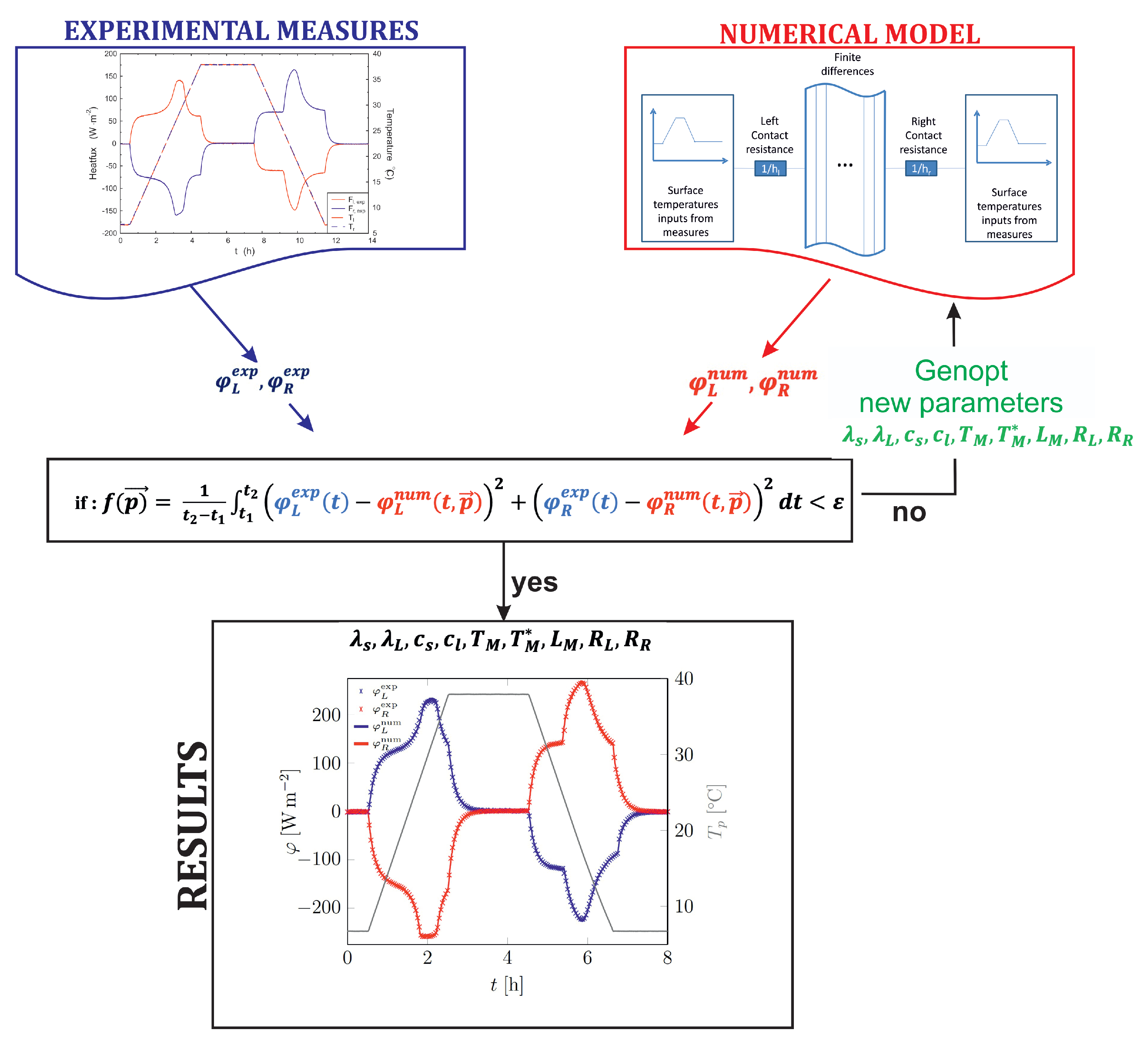
  • in recent studies, a more generic approach based on inversion methods has been developed in order to determine separately the main thermo-physical properties, such as the heat capacities (solid and liquid) and/or the latent heat etc. [36,52,65]. The main idea is to combine some experimental measurements, usually the temporal evolution of the heat-flow rate, with a numerical model of the composite sample. The correct values for the intrinsic parameters of the material are retrieved by minimizing an objective function.
In summary, there exist several methods to determine either the transport properties (conductivity and thermal resistances) or the thermodynamical ones (heat capacity, latent heat). Nonetheless, it is still difficult to first determine them altogether and second, both the repeatability and the final uncertainties quantifications on the average mascroscopic values are very scarce [34,36,40,45,52]. In this respect, the deviation for the thermal conductivity and specific capacity can vary from 1 to 12% and from 5 to 66% respectively in [34]. Similarly, [36] conclude that determinations of the apparent capacity in the range 10.43–19.4%, and 1.8% for the thermal conductivity, are acceptable for engineering use. On the other hand, [40] obtain a precision of 8% for the equivalent capacity, while [52] show results whose discrepancies are between 10% and 30%. Added to this, [45] highlight uncertainties of 10% for the thermal conductivity. To shed light on this brief landscape, it is worth recalling that current standards for the determination of PCM enthalpy functions are of the order of 10% [66,67].
Thus, the objective of the present work is to propose a non-intrusive extended method to characterize all the thermo-physical properties of a composite material composed of a cement mortar integrating a micro-encapsulated PCM. The intrinsic features are two-fold. First, all the required parameters are obtained altogether. Then, the needed parameters to perform simulations with dedicated tools (as EnergyPlus or Modelica for instance) are directly provided. Further, a painstaking and exhaustive analysis is carried out to study the scedasticity of the identified parameters. The goal is to prove the robustness and reliability of the method. Practically, the paper is organized as follows. The basic principle of the method is given in Section 2. In summary, it is composed of an experimental part followed by an identification one. The former one, whose protocole is defined in Section 2.1, involves a full sample of the composite material, i.e., at a real scale. This latter one is then thermally stimulated, at different heating and cooling rates, and it undergoes several cycles for each heat stress. The next step, detailed in Section 2.2 and Section 2.3, relies on an inverse method, which uses a numerical modeling of the sample. The physical modeling is first presented, its specificity being to impose a thermodynamically consistent approach, and then the numerical method is detailed. Features of the inverse process are finally given. In plain language, it combines the experimental measurements and the numerical results to identify the various thermo-physical parameters. In practice, both the transport and thermodynamical properties of the composite mortar and the thermal contact resistances are determined. Eventually, the main results are given in Section 3. As mentioned thereinbefore, several cycles of complete melting and solidification at various rates are completed. A first mortar is analyzed in Section 3.1, considering first a single thermal stress and then all the temperature ramps that have been set to the material. Then, the same analysis is performed for all the mortars altogether. Meanwhile, the scedasticity of the results is also performed, which has not been done before to the authors’ knowledge. Finally, the main conclusions are recalled in Section 4.

2. Method

The basic principle of the present study is thus to completely characterize a composite mortar thanks to an inversion process coupling the measurements done on the real experimental sample and the simulation of its behavior when submitted to a thermal stress. These three ingredients are detailed in the sequel, yet a synthetic flowchart is provided first in Figure 1. So, both the temperature and the heat flow-rate are measured on each side. Then, the former ones are used as boundary conditions for the numerical system, which computes the corresponding heat flow-rates. These latter are compared with the experimental ones, and a specific criterion is built to quantitatively check the agreement. If a large gap is observed, then the values of the thermo-physical parameters are modified, and the system is solved once again. When the method is converged, comparisons between the experiments and the calculations are built.

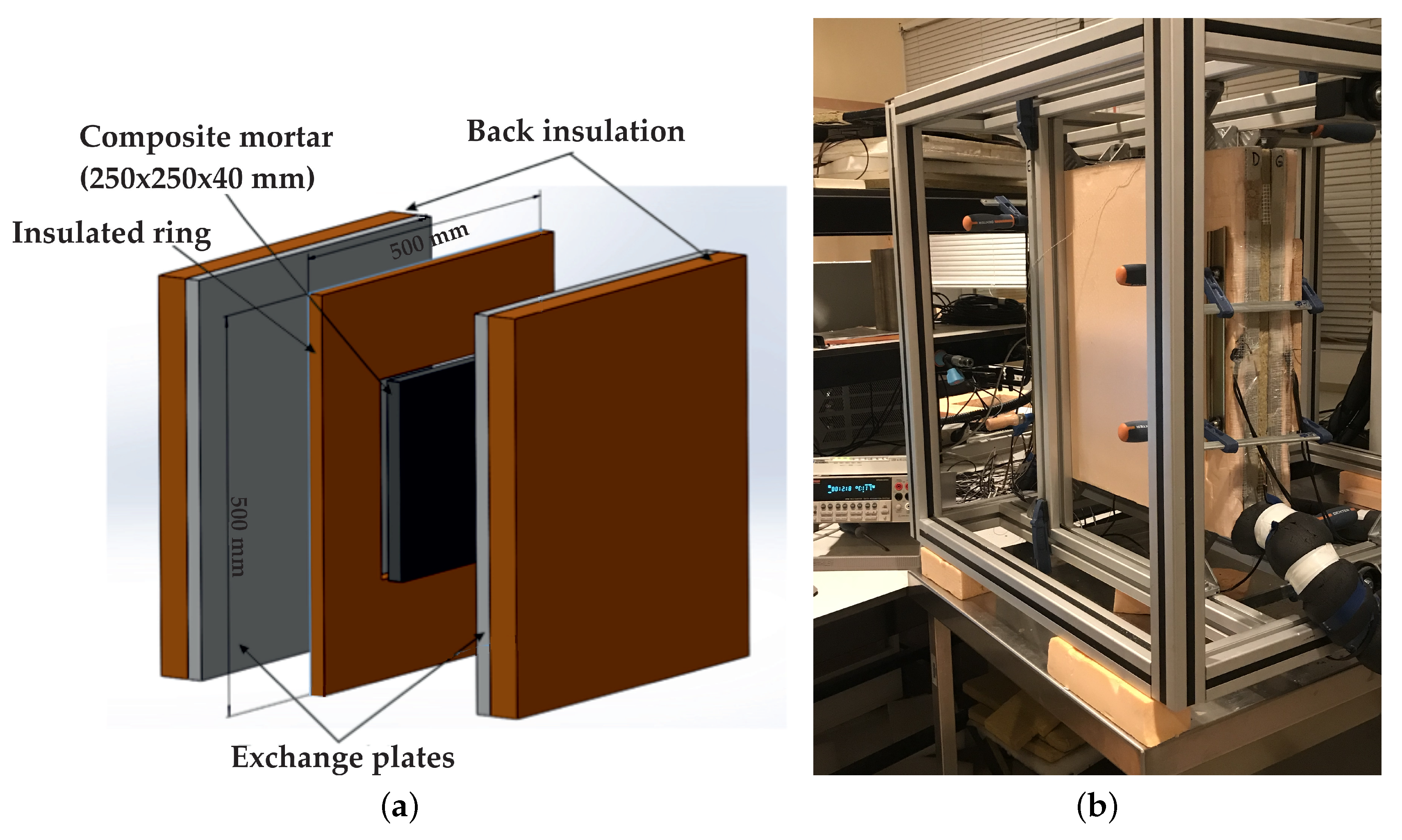
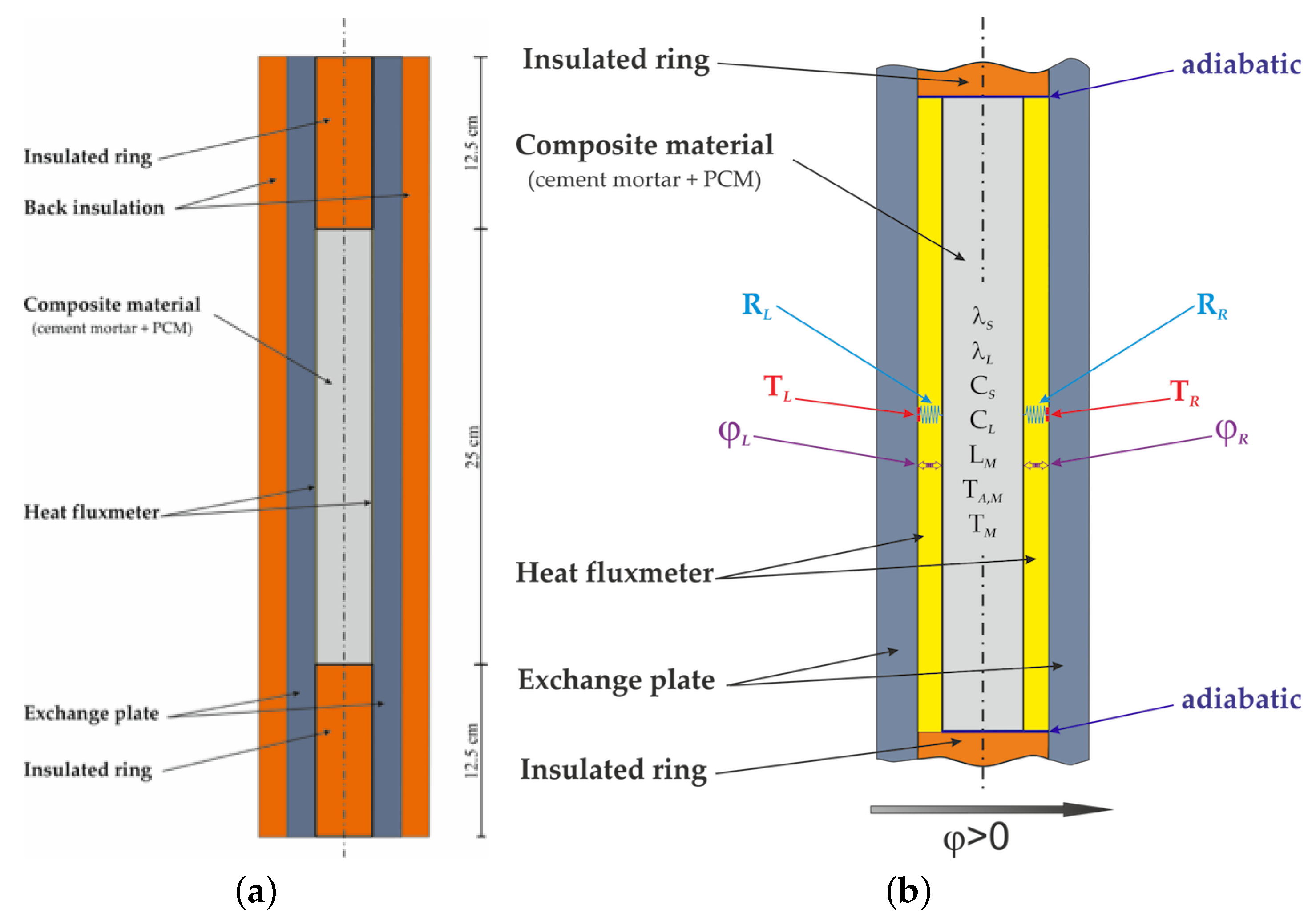
2.1. Experimental Protocol

As mentioned above, the present experimental protocol consists of the realization of several tests for different cement mortars including various amounts of PCM, the idea being to have the same ratio of cement/sand (here 1:2.6) in each mixture. At first, sand (siliceous rounded sand 0.4 m m ) and cement (CEM I 52.5 N complying with the EN 196–1 standard) are mixed in order to homogenize components with laboratory moisture content. Secondly, the PCM and water are added at the end of the mixing process in order to expose micro-capsules as short as possible to mechanical stress. The quantity of water added to make the composite mortars does not depend on the quantity of cement but rather on the quantity of PCM included, and it can be very significant due to the high specific surface of the micro-encapsulated PCM. The ratio of PCM estimated in each mixture is calculated using the mass of solid materials, i.e., sand, cement, and PCM. The water added is considered as the required water for the setting of mortar. Practically, to achieve a satisfactory workability, this needed water is dependent on the quantity of micro-capsules. Yet, the real needed water can not be controlled and therefore, free water is present in all samples. When drying, this later one will be replaced by cavities which are consequently different from one sample to another. Concretely, this implies that the dependency of some parameters (the density, the thermal conductivity, and the heat capacity) do not depend only on the PCM amount. Lastly, all associated densities for each material are furnished in Table 1. Three home-made composite mortars were realized in moulds of 250 × 250 × 40 m 3 and all samples have been dried in the laboratory over several months before being used for the experiments. The weight of samples was monitored before and after the tests. No noticeable variations have been seen, since the differences were of the same order as the precision of the scale ( 0.1 g ), which highlights a stable water content during the tests. Thus, the characteristics of the mortars studied are presented in Table 2, where each mortar is named according to its PCM mass percentage. Concretely, the previous compositions can also be given in mass of PCM per unitaire volume: this leads to the values of 175, 241.3, and 272 kg MCP / m 3 for each case, respectively.
The micro-encapsulated PCM used here for the home-made mortars is the well-known BASF’s Micronal® DS 5001 X, where the PCM is contained in the core of micro-capsules ranging from 2 μ m to 20 μ m in diameter. Practically, BASF claims that the micro-capsules are completely sealed, safe to process, and free of formaldehyde. It is also specified that the encapsulation process protects the wax in its very pure form, resulting in a high heat storage capacity of 110 k J kg 1 being permanently guaranteed. The melting point of Micronal® DS 5001 X, given by the manufacturer, is about 26 C . We realized the characterization of the PCM included in our composite materials with a pyris Diamond Perkin-Elmer DSC and we concluded that the latent heat is around 99 ± 10 k J kg 1 . This result is detailed within [68].
After the composite mortars have dried and hardened, the samples are placed in the experimental set-up, as depicted in Figure 2. First, the mortar is surrounded by an insulated ring. This ring avoids the heat losses by the lateral sides and enables 1D transfer towards the studied sample in the area of measures. On each face of the sample, a tangential gradient fluxmeter [69] with integrated thermocouples (T-type precalibrated at ± 0.1 C ) is stuck to limit the contact thermal resistance and measure both the heat flux and the temperature. Their dimensions are similar to those of the sample, which means that they are 250 × 250 mm2. Practically, these are CAPTEC products, whose thicknesses are about 0.2 mm and sensitivity are 120 μ V W 1 m 2 . The calibration procedure, described in [69,70], permits us to calibrate these sensors with a precision of ± 3 % as demonstrated for the example in [71]. Secondly, the entire sample is positioned between two exchange plates in order to impose the temperature on the two main faces. The plates are held compressed against the sample by means of clamps, as shown in Figure 2b.
Each exchange plate is linked, by an isolated pipe, to a thermoregulated bath, allowing control of the water temperature. Practically, a “snail” pattern is dug into each aluminum exchange plate, similarly to what is usually done with heating floor. The entrance and exit are close to each other. The incoming water circuit goes from the exterior to the center, and then the return flow paths from the inner to the outer side. The homogeneity of the temperature field has been checked with an infrared camera that shows that the temperature difference is less than 0.2 C , proving that the plate can be considered isothermal.
The temperature-controlled exchange plates are linked to thermoregulated baths, which themselves are managed by a computer. Featured later on in this work, the temperature of the exchange plates will be used as an input parameter (boundary condition) of the model and the heat flux measurements will be compared with the numerical model predictions. The boundary conditions and the parameters to identify are presented in Figure 3, where the thermal resistances R account for both the thermal contact resistance and the conductive resistance.
The experimental protocol consists of imposing different temperature ramps on the sample in order to completely melt and solidify the PCM inside the mortar. To be sure that it is completely fused or crystallized between melting or cooling ramps, a constant temperature step is applied between each ramp and the levels of these steps are chosen far above and below the phase change temperature. The required durations of these temperature steps are obtained when the sample reaches an isothermal state highlighted by the vanishing of the heat flow-rate. The various sensors are connected to a Keithley 2700 multichannel multimeter adapted to low level signals measurement.
Concretely, four heating/cooling durations have been tested (2, 3, 4, and 5 h ), and after a zeroth initial cycle, three cycles are realized and monitored for all samples. The corresponding temperature levels used are 5 C and 35 C .

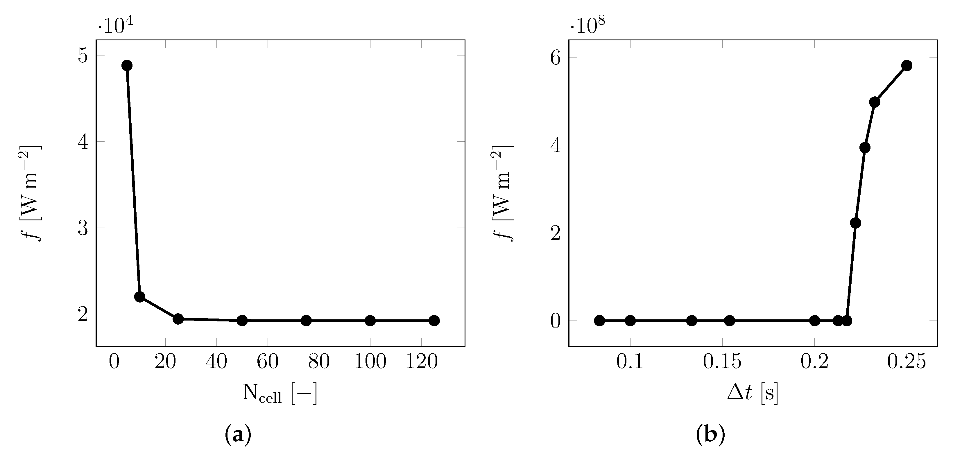
2.2. Numerical Method

Given the small size of the PCM inclusions and their homogeneous distribution into the solid cement mortar ( c m ) matrix, we model the sample as a homogeneous medium, characterized by macroscopic thermo-physical properties. According to the same principle, the latent heat of the inclusions is homogenized and allows to define an apparent latent heat of the homogeneous material. These assumptions also make it possible to consider only conduction transfers [68].
Thus, the physical model writes:
ρ d h d t = · ( λ T )
where all involved parameters are apparent ones.
Closure of (1) is then done by defining the initial and boundary conditions:
T = T 0
φ L num = T p , L T L R L
φ R num = T p , R T R R R
where T p is the temperature of the exchange plate and R the corresponding thermal resistances for the left and right side respectively, as shown in Figure 3b.
Finally, the enthalpy function h ( T ) is the one to be identified. Furthermore, the properties of the PCM are not constant, since they depend on its physical state (liquid or solid): consequently, the variation of the thermo-physical properties of the composite material depends on the liquid fraction χ of the PCM and involves its solid and liquid properties.
Moreover, the following assumptions are made:
  • The PCM being micro-encapsulated, the thermal expansion during the phase transition can be neglected, which implies that solid and liquid densities are equal.
    n.b. in such a case, there is no difference between the mass and volume fractions, which are therefore both denoted by χ .
  • The thermodynamic behavior of the PCM, i.e., its enthalpy function, obeys a binary solution model [68]:
    d χ = T M T M T M T 2 d T
    d h d T = T M T M T M T 2 L M ( T ) + c s 1 T M T M T M T + c l T M T M T M T
    Here, the involved latent heat for the composite mortar depends on the mass fraction Y of the PCM included in this latter one:
    L M = Y L M
  • The thermal conductivity is governed by a classic average [72,73,74]:
    λ = χ λ l + ( 1 χ ) λ s
    where indices s and l stand for the homogeneous material, that is to say to the initial cement mortar with the liquid or solid contribution of the PCM.
Lastly, the system of partial differential equations described by Equations (1) and (2) is solved numerically using a finite-volume method, based on a first-order scheme for the flux calculations and on an Euler integration. The mesh used contains 100 cells, which corresponds to a space step of 0.4 m m , and the time step is fixed at 0.1 s . These parameters have been set after a convergence study, presented in Figure 4, which has shown that the solution was not sensible to further refinement.

2.3. Inversion Process

In summary, several experiments have been done and, given a thermal program, various heat flow-rates have been measured during time. Further, a numerical model has been built so as to compute the numerical heat-flow rate for a given set of input parameters p ; that is to say for different values of the thermodynamic and thermal properties, i.e., for a given p = λ s , λ l , c s , c l , T M , T M , L M , R L , R R . These nine parameters correspond to the thermodynamical ones associated with the phase change, and to the heat transfers ones with the thermal conductivities of the material, as well as the thermal contact resistances on both sides. They are determined during transient heating and cooling modes, involving both fusion and solidification.
Given these two data, i.e., the experimental and numerical heat flow-rates, a criterion can be defined in order to assess the correctness of the estimation of p , here thanks to the classic least-square error:
f ( p ) = 1 t 2 t 1 t 1 t 2 φ L exp ( t ) φ L num ( t , p ) 2 + φ R ext ( t ) φ R num ( t , p ) 2 d t
The basic principle of the inversion step is thus to minimize this cost function f over p , which can be done in different ways, as for instance using a simplex approach [75] or a Levenberg–Marquardt method [76] or genetic algorithms [77,78].
In the present case, the identifications were performed using the GenOpt free tool from the Lawrence Berkeley National Laboratory [79,80]. It indeed implements several classic algorithms, including the ‘GPSCoordinateSearch’ that has been used here: the basic principle of the generalized pattern search (GPS) is to link monodimensional minimizations according to the different directions of the search space (dimension N). The version implemented in GenOpt automatically adapts the search accuracy to obtain an acceptable solution without requiring too much computation time. As any optimization method, GenOpt requires to define all the N parameters to be identified ( p R N ) so as to minimize the cost function f ( p ) : R N R given by relation (6). Let us mention here that GenOpt always delegates the evaluation of the cost function f to an external program, which corresponds here to the code implementing the aforementioned system of PDE. From a practical point of view, the raw text files that ensure the communication between these two threads are configured following the documentation [81]. As a rule of thumb, all identified parameters are described by their name, used only for display purpose, and by an initial value (first guess), as well as by lower and upper bounds. As an example, the latent heat and solid thermal conductivity are initialized, respectively, at 16.5 k J kg 1 and 0.4 W K 1 m 1 , and their minimal and maximal authorized values are 14 and 18 k J kg 1 , and 0.3 and 0.5 W K 1 m 1 . Moreover, each run is repeated three times: in one case, the initial seed is set by the user, and in the two others, they are randomly chosen inside the search space. In these latter cases, it is obviously checked that the chosen first guess will lay inside the respective bounds defined hereinbefore.
Finally, since the iterative algorithm always starts from an initial estimation p 0 arbitrarily chosen, it can occur that the algorithm converges towards a local minimum. To avoid this caveat, GenOpt therefore proposes to re-launch the same optimization several times (three times in this work) by randomly selecting the initial estimate in the search space: this lengthens computation times but increases the chances of converging towards the global minimum.

3. Results

The results obtained after the 192 optimizations are now presented. Firstly, a focus is done on the 12.4 % w -PCM mortar, considering only the first cycle of the 2 h ramp experiment, and then all the other cycles. Secondly, the analysis is produced for all the samples, considering here all ramps and all corresponding cycles. A statistical survey is done on all the results, together with a comparison of the final identified values for the thermal and thermodynamic parameters. Finally, the identified enthalpy functions are compared altogether and the total error is shown.
n.b. The results after identification are gathered in Appendix A for the sake of clarity and only the main ones are presented below.
Furthermore, as mentioned before, the amount of initial water necessary for the cement hydration and the amount of extra free water influence the porosity of each mortar. Concretely, this latter one impacts the macroscopic properties, as for instance the densities, the thermal conductivities, and the heat capacities. In contrast, the latent heat will not be affected by this effect. Nevertheless, the relation between the porosity and the evolution of the equivalent characteristics of the composite mortars is out of the scope of the present work, which mainly focuses on the identification of these properties in function of the amount of PCM.

3.1. First Sample

As mentioned hereinbefore, the starting point is the first cycle of the 2 h ramp for the 12.4 % w -PCM mortar. The experimental heat flow-rates on the left and right sides of the sample for the given imposed temperature ramp are shown in Figure 5 with the corresponding numerical heat flow-rates obtained after the inversion process. One can see that agreement between the experimental measurements and the numerical computations is very good. Then, an obvious asymmetry is observed between each sides. This can be easily explained by the fact that, experimentally, the thermal contact is not perfect and is always different from one face to the other since their roughness is different. Consequently, huge variations can arise between these two sides. Yet, in spite of this asymmetry, the method is capable of reproducing the experimental behavior without any difficulties. Moreover, it is worth mentioning that the real sample also shows a non-symmetrical behavior between the melting and the crystallization steps, which is perfectly captured by the numerical calculation. This remark has to be further commented. First, this behavior is not due to the presence of supercooling, which would lead to a clear discontinuity during cooling, which is not observed experimentally. Added to this, it would be rather difficult for the results to represent such a phenomenon since it has not been considered during the modeling. In fact, this asymmetric feature is obtained only because the enthalpy function is governed by the relation (3), which shows a different behavior when going to the solid to liquid state and vice-versa. In other words, the slope of the function (and so its derivative) being non-constant, dynamics of the phase transition is different between melting and solidification. In this respect, this means that any enthalpy function having a symmetrical expression, as for instance with pure substances or solutions where a linear profile is assumed between the liquidus and the solidus, will no be capable to reproduce such a behavior. Once again, this is possible if and only if enthalpy function obeys Equation (3), as demonstrated in [68].
Eventually, the corresponding enthalpy function is depicted in Figure 6 and the values for the associated parameters, obtained after identification, are given hereafter:
c S = 1094 J K 1 kg 1
c L = 1094 J K 1 kg 1
T M = 25.57 C
T M = 27.18 C
L M = 12,322 J kg 1
Here again, some discussion is needed. Indeed, in the inversion process, it is important to recall that an unique enthalpy function is determined. So, with a single expression, obeying a non-symmetrical formulation as discussed above, the behavior of the material is described for both the solid and the liquid state. Consequently, this obviates the usual formulations assuming one expression for the heating and another for the cooling, which is indisputably inconsistent with basic thermodynamic laws, as further discussed in [62].
After this study for the first cycle, the purpose is extended to the other cycles of the 2 h ramp experiment. Thus, the second and third cycles are used as original inputs in the inversion process, as well as the entire set of cycles. The corresponding results are furnished in Figure 7. In all cases, the numerical results obtained with the present procedure show a very good agreement with the experimental data. Once again, both the non-equal thermal contact resistances at the left and right sides and the asymmetrical behavior between the fusion and solidification are perfectly rendered by the computations. Eventually, the enthalpy functions obtained after the inversion process are depicted in Figure 8. In Figure 8a–d the enthalpy functions obtained when using either the first or second or third or all cycles as original inputs are shown. Then, in Figure 8e, all these inverse results are compared with each other. On this latter one, it is worth noticing that the four estimated curves agree very well and cannot be distinguished from each other. From a practical point of view, this means that the cycle used for the inversion process is completely pointless. In other words, the method always permits to obtain the same results, i.e., an unique enthalpy function, whatever the original experimental measures used to initiate the seeds points of the inverse method. Undeniably, this is in complete agreement with thermodynamic laws.

3.2. All Samples

Given the previous results, it is now proposed to analyze all the available experiments. Thereby, all mortars are studied for the four different heating/cooling ramps each time, the inversion process using all the cycles (first to third) to identify the enthalpy function. As said before, only the final results will now be presented, yet all the values can be found in Appendix A.
Thus, the enthalpy functions obtained after the inversion step are shown in Figure 9 and Figure 10, in function of the heating/cooling ramp and the type of mortar, respectively. In the first case, one can easily remark that, the higher the amount of PCM incorporated in the mortar, the higher the value of the latent heat. Practically, this increase is characterized by a larger phase change domain, situated between the two linear parts corresponding to the sensible states. Moreover, one can see that the beginning of this transition zone is almost the same for all mortars, whatever the heating rate that is used. In the second case, it is straightforward to notice that, for a given mortar, all the identified enthalpy functions collapse on a single curve. In other words, for all the heating rates and whatever the cycle that is used, or even if all of them are considered in the characterization process, the estimated enthalpy functions are not dependent on the heating ramp. In contrast with all the other existing methods, the present approach thus does not suffer from any non physical dependency of the enthalpy with the thermal stress. To further highlight this statement, the minimal and maximal and average values for all identified parameters are presented in Table 3 for each mortar. Concerning the thermodynamical parameters which are involved in the enthalpy relation (3), that is to say c s , c l , T M , T M , and L M , one can see that discrepancies are very low. Furthermore, when comparing the intensive parameters, that must not depend on the amount of PCM in the mortar, it is interesting to note that the maximum gap between the identified values is 0.26 C and 0.72 C for T M and T M , respectively, the associated deviation being 0.6% and 1.4%. In fact, these differences being of the order of the temperature uncertainty, one can conclude that all the numerical estimations coincide altogether. When looking at the other parameters, that vary with the amount of PCM, the comparisons can not be done anymore between all the mortars. Nonetheless, for a given mortar, the agreement between all the estimations is excellent.
Finally, a last comparison is proposed to clearly show the coherence between all the identified enthalpy functions. Knowing the minimal and maximal values for all the parameters, it is possible to build two extreme estimations for the enthalpy function. Such curves are given in Figure 11. Meanwhile, an error criterion between these curves is represented, which has been defined as follows so as to be non-dimensional:
ε = | h max h min | L M
It is obvious that, even when taking the extreme values for each parameter, the corresponding discrepancy is very low. In fact, it is clearly far below the usual accepted quality threshold which is currently around 10% [66,67].
Then, another analysis is proposed to clearly underline the possibility of the present method and its intrinsic strengthes. When looking at the other similar studies, summarized in Table 4, it appears that only five of them use the same PCM as in the present study. Besides, as stated before, some of them only deal with DSC [40,45,82] and the properties of a real macroscopic sample are addressed solely by [35], although only the thermal conductivity is involved in the latter paper. More importantly, when dealing with the thermal conductivity, very often, only an overall or effective value is furnished and no distinction is done between the concrete with PCM in solid or in liquid state, contrary to what is currently done here.
So, similarly to what has been found by [35,45], it can be seen in Figure 12 that the inclusion of PCM leads to a decrease of the thermal conductivity. Furthermore, a value of 0.4 W K 1 m 1 has been estimated in the 14.5% w case by [35], which is pretty close to the corresponding present cases (12.4% w and 19.2% w ) with λ s = 0.602 ± 3.74 % W K 1 m 1 and λ l = 0.592 ± 2.86 % W K 1 m 1 , and λ s = 0.43 ± 2.03 % W K 1 m 1 and λ l = 0.441 ± 3.54 % W K 1 m 1 . In the same way, [45] obtained values of 0.49 0.5 W K 1 m 1 and 0.42 0.48 W K 1 m 1 with 10% w and 20% w , while the current 12.4% w and 22.1% w cases lead to λ s = 0.602 ± 3.74 % W K 1 m 1 and 0.383 ± 0.58 % W K 1 m 1 , and to λ l = 0.592 ± 2.86 % W K 1 m 1 and 0.386 ± 1.74 % W K 1 m 1 , respectively. In the same idea, the identified specific heat capacities are depicted in Figure 13. Due to the large discrepancies between all the data, no quantitative comparison can be done yet the results agree qualitatively, nevertheless, we can note that the present values are very close to each other. Lastly, by dividing the current latent heats obtained for each mortar, in Table 3, by the mass fraction of the PCM, one can express the latent heat in function of the specific mass of the PCM instead of the one of the mixture (cement+PCM). More clearly, this means that the latent heat of the PCM can be directly calculated and, then, compared to the experimental value of 99 k J kg 1 , which was determined by DSC [68]. This measurement had been down with a Pyris Diamond apparatus from Perkin Elmer, using a 5.78 m g sample and a 5 K min 1 heating rate on dynamic mode. The corresponding results are shown in Table 5: once again, the agreement with the experimental measure is very good, a standard deviation of 3.56% being observed for a mean value of 95.47 k J kg 1 . The associated discrepancy with the experimental measurement is of 1.23%, which is excellent given all the experimental and numerical uncertainties.
Eventually, another aspect of the inversion procedure is going to be analyzed by considering the identified values for the thermal parameters, that is to say the thermal conductivities and the thermal resistances furnished in Table 3. One can see that the former ones are pretty well estimated, the discrepancy being several orders below the usual uncertainties for PCM measurements. In contrast, the determination of the thermal resistances is more tricky, which is very well known. These depend on the surface state and therefore the thermal contact resistance between the material and the sensor (heat fluxmeter). The advantage here is that these resistances are estimated on each side and for each sample. Hopefully, the behavior of the mortar is mainly governed by the latent effects and consequently this lack of precision does not impact the inversion process when identifying the thermodynamical parameters, as seen above. However, it is clear that no good estimations of the thermal conductivity can be achieved if this problem is not addressed carefully.

4. Conclusions

The goal of this work is to present an efficient method for characterizing the thermo-physical properties of a composite material, which is in the present case a cement mortar containing a micro-encapsulated PCM, as it could be used in real conditions. These properties are the required parameters for the development of a numerical model able to reliably representing the thermal behavior of the material containing phase change material.
The first step of the study is based on an experimental device where the material to be characterized is repeatedly stressed by temperature ramps, at various speeds, in order to carry out several cycles of melting/crystallization of the PCM. This fluxmetric device allows simultaneous measurements of heat fluxes and temperatures to the access faces of the material during these successive thermal stresses. These non-intrusive measurements, essential for the characterization of the composite material, are then used as boundary conditions of a numerical model detailed hereafter.
In a second step, a physical model is developed to reproduce both the thermal and thermodynamic behavior of each sample. In practice, it is thus necessary to impose a thermodynamically consistent formulation of the enthalpy h ( T ) , represented in the present case as a binary solution. This function h ( T ) implemented in the numerical model, developed in a finite-volume framework, makes it possible to account for the non-symmetrical thermal response of the samples submitted to heating and cooling stresses (i.e., fusion and solidification).
The last step is to combine together in an inverse method the experimental measurements with the numerical results obtained when solving the physical model. The use of efficient optimization methods allows a reliable estimation of the thermo-physical properties of the composite material, integrating the accuracy of the experimental measurements, and the thermodynamical correctness of the modeling. These thermo-physical parameters stand here for the thermal conductivities and heat capacities when the PCM is in the solid or liquid state on one hand, and the temperatures defining the transition range and the corresponding latent heat on the other hand.
Concretely, the identification of the parameters is done simultaneously for each of the three cycles and then altogether with the inversion method. In order to thoroughly test the method, the studies are conducted on several melting/solidification cycles for three mortars incorporating different amounts of PCM. The results obtained show a very low dispersion, less than 3% and 4% for thermal conductivities and heat capacities, respectively, 2% (0.5K) for T, 3% for L M , and 4% for the complete enthalpy curve. These results are excellent considering the current standards, which are usually advanced as 1K for T M and 10% for L M [66,67]. Moreover, the masses of PCM integrated in the mortar as well as the speeds of thermal ramps do not affect the estimate of the transition temperatures, depending solely on the nature of the PCM which is similar from one sample to another. This independence is obviously in accordance with the laws of thermodynamics.
In addition, by taking into account the thermal contact resistances between the sensor and the samples, different from one side to another and dependent on the surface finishing and assembly (i.e., variable of a sample to another), do not pose any difficulty but, more importantly, improves the accuracy of the results. In contrast, if ignored, it would be equivalent to a direct method, and consequently, the estimated thermal conductivities would be erroneous.
Concerning the prospect of this work, it concerns the studies of more complex PCMs which cannot be described by a binary model but need more sophisticated thermodynamics. This could finally be one of the main limitation of the present method since it can only determine the values of already known parameters. Saying this differently, one has to know or assume the thermodynamical expression of the enthalpy function. In such a case, the problem can be manyfold. The principal issue will be to find the correct formulation for the equation governing the enthalpy function, specifically if many components are contained in the mixture. Then the numbers of parameters to be identified could probably increase and therefore the computational cost increases. Finally, It should also be noted that, in the present case, the PCM does not show supercooling phenomena, which is cumbersome to consider if required.

Author Contributions

Conceptualization, L.Z., E.F., S.G.; methodology, L.Z., E.F., S.G.; validation, L.Z., E.F., S.G., P.T., D.D.; investigation, L.Z., E.F., S.G., P.T., D.D.; resources, E.F.; writing—original draft preparation, E.F.; writing—review and editing, L.Z., E.F., S.G., P.T., D.D., visualization, E.F.; supervision, L.Z., E.F.

Funding

This research received no external funding.

Conflicts of Interest

The authors declare no conflict of interest.

Nomenclature

Latin symbols
cspecific heat capacity, J K 1 kg 1
Dduration, h
ethickness, m
fcost function, W 2 m 4
hspecific enthalpy, J kg 1
Llatent heat, J kg 1
p set of parameters, −
Rthermal resistance, W 1 K m 2
Ttemperature, C
ttime, s or min
X vector of coordinates, m
Ymass fraction of PCM, −
Greek symbols
ε error, %
φ heat flux, W m 2
λ thermal conductivity, W K 1 m 1
ρ density, k g m 3
χ liquid fraction, −
Subscripts and superscripts
pure component (solvent phase)
e x execution
exp experimental
Lleft
lliquid
Mmelting
num numerical
pexchange plate
Rright
ssolid
wweight
Acronyms
DSCdifferential scanning calorimetry
GPSgeneralized pattern search
PCMphase change material

Appendix A. Additional Data

In order to help the possible interested readers to re-analyze the data or to propose new post-treatments, all results are given hereinafter. Thus, the values of the identified parameters for every heating/cooling ramps are furnished in Table A1, Table A2 and Table A3 for the 12.4 % w - and 19.2 % w - and 22.1 % w -PCM mortar, respectively. Then, the comparisons between the experimental measurements and the numerical results are shown in Figure A1, Figure A2, Figure A3, Figure A4, Figure A5, Figure A6, Figure A7, Figure A8, Figure A9, Figure A10 and Figure A11. Here, all cases are given, that is to say for each mortar and each associated heating/cooling ramp with all the possible cycles (first, second, third, or alltogether) as initial inputs for the inversion process. Finally, the corresponding identified entalphy functions are depicted in Figure A12, Figure A13 and Figure A14.
Table A1. 19.2%w-PCM mortar: values of the identified parameters for each heating/cooling ramp and for the first, second, third, and all cycles together cases.
DfRLRRλsλlcsclTM T M LMtex
22,5771.098 · 10−24.638 · 10−30.6060.61094109425.5727.1812,3220:22:39
2 h22,5961.085 · 10−24.39 · 10−30.5940.5891094109425.5727.1712,3171:05:41
23,0281.084 · 10−24.39 · 10−30.5940.5891100109425.5827.1712,2671:12:19
68,1751.084 · 10−24.412 · 10−30.5940.5891094109425.5727.1712,3220:56:43
20,4031.125 · 10−24.737 · 10−30.5940.5891089108925.5727.1712,4782:05:37
3 h19,8991.154 · 10−25.028 · 10−30.6110.61089108925.5827.1912,4612:06:14
19,7741.139 · 10−24.918 · 10−30.6060.5941094109425.5427.0912,2942:05:01
59,3371.139 · 10−24.891 · 10−30.6060.5941089109425.5627.1412,4001:45:29
18,0951.111 · 10−25 · 10−30.60.5891094109425.5327.0612,3282:27:47
4 h18,6421.111 · 10−24.918 · 10−30.5940.5831089109425.5427.1112,4220:44:17
18,2301.125 · 10−25 · 10−30.60.5891094109425.5327.0712,3282:50:45
55,7931.111 · 10−24.891 · 10−30.5940.5831089109425.5427.1112,4222:05:56
17,8211.2 · 10−25.455 · 10−30.6060.5941094109425.5327.0312,3004:12:57
5 h17,9241.2 · 10−25.455 · 10−30.6060.5941094109425.5227.0112,2834:31:10
17,5181.216 · 10−25.625 · 10−30.6170.61089109425.5427.0812,3611:20:27
52,8451.2 · 10−25.455 · 10−30.6060.5941094109425.522712,2613:28:31
Table A2. 19.2%w-PCM mortar: values of the identified parameters for each heating/cooling ramp and for the first, second, third, and all cycles together cases.
DfRLRRλsλlcsclTM T M LMtex
30,3131.159 · 10−23.127 · 10−20.4350.4421096103525.5927.3118,13501:43:24
2 h23,3901.224 · 10−23.14 · 10−20.4310.4361067103725.5727.2818,23300:50:28
21,8591.24 · 10−23.127 · 10−20.4310.4361069103625.5827.2818,16800:59:37
85,8781.204 · 10−23.127 · 10−20.4310.4371074103525.5927.3418,27902:16:47
20,7851.304 · 10−23.176 · 10−20.4270.4371062103525.727.5118,35206:43:38
3 h20,5511.321 · 10−23.189 · 10−20.4270.4361065103125.6827.4318,24108:27:05
21,6971.33 · 10−23.189 · 10−20.4280.4381067103025.6927.4618,26510:36:33
61,9061.313 · 10−23.176 · 10−20.4260.4361066103225.6927.4718,27308:26:34
19,0511.399 · 10−23.24 · 10−20.4270.4431062103125.7627.5918,34313:48:26
4h19,2161.397 · 10−23.24 · 10−20.4280.4421067103125.7427.5418,20711:21:10
19,2161.397 · 10−23.24 · 10−20.4280.4421067103125.7427.5418,20708:59:56
57,0621.399 · 10−23.24 · 10−20.4270.4421065103125.7527.5718,27008:19:15
18,0941.434 · 10−23.266 · 10−20.4290.4431073103525.7727.5417,97810:20:06
5 h19,1701.467 · 10−23.293 · 10−20.4330.451066103225.7827.6118,19006:04:20
18,6791.473 · 10−23.306 · 10−20.4330.4511063103125.7827.6318,26006:47:33
56,0061.465 · 10−23.293 · 10−20.4330.4491064103225.7827.6318,22207:19:31
Table A3. 22.1%w-PCM mortar: values of the identified parameters for each heating/cooling ramp and for the first, second, third, and all cycles together cases.
DfRLRRλsλlcsclTM T M LMtex
17,5117.893 · 10−31.364 · 10−20.3840.3841154108825.5226.9120,67900:54:19
2 h18,8997.825 · 10−31.364 · 10−20.3840.3841151108425.5226.9420,77804:15:25
21,1837.826 · 10−31.364 · 10−20.3820.3821137108425.5427.0221,0273:43:08
57,9357.895 · 10−31.364 · 10−20.3840.3841150108725.5226.9320,7578:31:31
21,0148.333 · 10−31.429 · 10−20.3840.3871132108125.7227.3721,33618:28:41
3 h20,9158.257 · 10−31.429 · 10−20.3820.3871142108125.6327.1921,09441:58:24
23,8508.333 · 10−31.429 · 10−20.3840.3871153108125.6227.120,84810:45:50
66,0278.333 · 10−31.429 · 10−20.3840.3891144108325.6627.2121,05240:53:30
28,6808.571 · 10−31.452 · 10−20.3820.3841144108125.6727.2621,05342:29:36
4 h26,6418.654 · 10−31.452 · 10−20.3840.3871151108125.6727.2320,983108:57:29
25,3238.571 · 10−31.452 · 10−20.3820.3871144108225.6727.2621,06732:22:59
80,7898.571 · 10−31.452 · 10−20.3820.3871146108125.6727.2621,07959:49:49
28,3228.824 · 10−31.475 · 10−20.3840.3871160108625.6727.1620,6829:59:39
5 h26,5488.738 · 10−31.475 · 10−20.3820.3871159108425.6727.220,76344:44:31
27,8898.654 · 10−31.475 · 10−20.3820.3871163108725.6727.1620,58713:43:08
80,4198.738 · 10−31.475 · 10−20.3820.3871147108625.6927.2821,00074:28:11
Figure A1. 12.4%w-PCM mortar: comparisons of the experimental fluxes with the numerical ones after identification for the 3 h heating/cooling ramp experiment.
Applsci 09 01104 g0a1
Figure A2. 12.4%w-PCM mortar: comparisons of the experimental fluxes with the numerical ones after identification for the 4 h heating/cooling ramp experiment.
Applsci 09 01104 g0a2
Figure A3. 12.4%w-PCM mortar: comparisons of the experimental fluxes with the numerical ones after identification for the 5 h heating/cooling ramp experiment.
Applsci 09 01104 g0a3
Figure A4. 19.2%w-PCM mortar: comparisons of the experimental fluxes with the numerical ones after identification for the 2 h heating/cooling ramp experiment.
Applsci 09 01104 g0a4
Figure A5. 19.2%w-PCM mortar: comparisons of the experimental fluxes with the numerical ones after identification for the 3 h heating/cooling ramp experiment.
Applsci 09 01104 g0a5
Figure A6. 19.2%w-PCM mortar: comparisons of the experimental fluxes with the numerical ones after identification for the 4 h heating/cooling ramp experiment.
Applsci 09 01104 g0a6
Figure A7. 19.2%w-PCM mortar: comparisons of the experimental fluxes with the numerical ones after identification for the 5 h heating/cooling ramp experiment.
Applsci 09 01104 g0a7
Figure A8. 22.1%w-PCM mortar: comparisons of the experimental fluxes with the numerical ones after identification for the 2 h heating/cooling ramp experiment.
Applsci 09 01104 g0a8
Figure A9. 22.1%w-PCM mortar: comparisons of the experimental fluxes with the numerical ones after identification for the 3 h heating/cooling ramp experiment.
Applsci 09 01104 g0a9
Figure A10. 22.1%w-PCM mortar: comparisons of the experimental fluxes with the numerical ones after identification for the 4 h heating/cooling ramp experiment.
Applsci 09 01104 g0a10
Figure A11. 22.1%w-PCM mortar: comparisons of the experimental fluxes with the numerical ones after identification for the 5 h heating/cooling ramp experiment.
Applsci 09 01104 g0a11
Figure A12. 12.4%w-PCM mortar: comparisons of the identified enthalpy functions with respect to the heating/cooling ramp (n.b. unique formulation pertaining for both fusion and crystallization).
Applsci 09 01104 g0a12
Figure A13. 19.2%w-PCM mortar: comparisons of the identified enthalpy functions with respect to the heating/cooling ramp (n.b. unique formulation pertaining for both fusion and crystallization).
Applsci 09 01104 g0a13
Figure A14. 22.1%w-PCM mortar: comparisons of the identified enthalpy functions with respect to the heating/cooling ramp (n.b. unique formulation pertaining for both fusion and crystallization).
Applsci 09 01104 g0a14

References

  1. Ürge-Vorsatz, D.; Cabeza, L.F.; Serrano, S.; Barreneche, C.; Petrichenko, K. Heating and cooling energy trends and drivers in buildings. Renew. Sustain. Energy Rev. 2015, 41, 85–98. [Google Scholar] [CrossRef]
  2. Serrano, S.; Ürge-Vorsatz, D.; Barreneche, C.; Palacios, A.; Cabeza, L.F. Heating and cooling energy trends and drivers in Europe. Energy 2017, 119, 425–434. [Google Scholar] [CrossRef]
  3. Zhu, N.; Ma, Z.; Wang, S. Dynamic characteristics and energy performance of buildings using phase change materials: A review. Energy Convers. Manag. 2009, 50, 3169–3181. [Google Scholar] [CrossRef]
  4. Tyagi, V.; Kaushik, S.; Tyagi, S.; Akiyama, T. Development of phase change materials based microencapsulated technology for buildings: A review. Renew. Sustain. Energy Rev. 2011, 15, 1373–1391. [Google Scholar] [CrossRef]
  5. Pomianowski, M.; Heiselberg, P.; Zhang, Y. Review of thermal energy storage technologies based on PCM application in buildings. Energy Build. 2013, 67, 56–69. [Google Scholar] [CrossRef]
  6. Konuklu, Y.; Ostry, M.; Paksoy, H.O.; Charvat, P. Review on using microencapsulated phase change materials (PCM) in building applications. Energy Build. 2015, 106, 134–155. [Google Scholar] [CrossRef]
  7. Khadiran, T.; Hussein, M.Z.; Zainal, Z.; Rusli, R. Advanced energy storage materials for building applications and their thermal performance characterization: A review. Renew. Sustain. Energy Rev. 2016, 57, 916–928. [Google Scholar] [CrossRef]
  8. Kasaeian, A.; bahrami, L.; Pourfayaz, F.; Khodabandeh, E.; Yan, W.M. Experimental studies on the applications of PCMs and nano-PCMs in buildings: A critical review. Energy Build. 2017, 154, 96–112. [Google Scholar] [CrossRef]
  9. Cabeza, L.; Castell, A.; Barreneche, C.; de Gracia, A.; Fernández, A. Materials used as PCM in thermal energy storage in buildings: A review. Renew. Sustain. Energy Rev. 2011, 15, 1675–1695. [Google Scholar] [CrossRef]
  10. Heier, J.; Bales, C.; Martin, V. Combining thermal energy storage with buildings—A review. Renew. Sustain. Energy Rev. 2015, 42, 1305–1325. [Google Scholar] [CrossRef]
  11. Stritih, U.; Butala, V. Energy saving in building with PCM cold storage. Int. J. Energy Res. 2007, 31, 1532–1544. [Google Scholar] [CrossRef]
  12. Waqas, A.; Din, Z.U. Phase change material (PCM) storage for free cooling of buildings—A review. Renew. Sustain. Energy Rev. 2013, 18, 607–625. [Google Scholar] [CrossRef]
  13. Kamali, S. Review of free cooling system using phase change material for building. Energy Build. 2014, 80, 131–136. [Google Scholar] [CrossRef]
  14. Akeiber, H.; Nejat, P.; Majid, M.Z.A.; Wahid, M.A.; Jomehzadeh, F.; Famileh, I.Z.; Calautit, J.K.; Hughes, B.R.; Zaki, S.A. A review on phase change material (PCM) for sustainable passive cooling in building envelopes. Renew. Sustain. Energy Rev. 2016, 60, 1470–1497. [Google Scholar] [CrossRef]
  15. Souayfane, F.; Fardoun, F.; Biwole, P.H. Phase change materials (PCM) for cooling applications in buildings: A review. Energy Build. 2016, 129, 396–431. [Google Scholar] [CrossRef]
  16. Islam, M.; Pandey, A.; Hasanuzzaman, M.; Rahim, N. Recent progresses and achievements in photovoltaic-phase change material technology: A review with special treatment on photovoltaic thermal-phase change material systems. Energy Convers. Manag. 2016, 126, 177–204. [Google Scholar] [CrossRef]
  17. Shukla, A.; Buddhi, D.; Sawhney, R. Solar water heaters with phase change material thermal energy storage medium: A review. Renew. Sustain. Energy Rev. 2009, 13, 2119–2125. [Google Scholar] [CrossRef]
  18. Abokersh, M.H.; Osman, M.; El-Baz, O.; El-Morsi, M.; Sharaf, O. Review of the phase change material (PCM) usage for solar domestic water heating systems (SDWHS). Int. J. Energy Res. 2017, 42, 329–357. [Google Scholar] [CrossRef]
  19. Moreno, P.; Solé, C.; Castell, A.; Cabeza, L.F. The use of phase change materials in domestic heat pump and air-conditioning systems for short term storage: A review. Renew. Sustain. Energy Rev. 2014, 39, 1–13. [Google Scholar] [CrossRef]
  20. Kapsalis, V.; Karamanis, D. Solar thermal energy storage and heat pumps with phase change materials. Appl. Therm. Eng. 2016, 99, 1212–1224. [Google Scholar] [CrossRef]
  21. Tyagi, V.V.; Buddhi, D. PCM thermal storage in buildings: A state of art. Renew. Sustain. Energy Rev. 2007, 11, 1146–1166. [Google Scholar] [CrossRef]
  22. Zhang, Y.; Zhou, G.; Lin, K.; Zhang, Q.; Di, H. Application of latent heat thermal energy storage in buildings: State-of-the-art and outlook. Build. Environ. 2007, 42, 2197–2209. [Google Scholar] [CrossRef]
  23. Baetens, R.; Petter Jelle, B.; Gustavsen, A. Phase change materials for building applications: A state-of-the-art review. Energy Build. 2010, 42, 1361–1368. [Google Scholar]
  24. Kuznik, F.; David, D.; Johannes, K.; Roux, J.J. A review on phase change materials integrated in building walls. Renew. Sustain. Energy Rev. 2011, 15, 379–391. [Google Scholar]
  25. Zhou, D.; Zhao, C.; Tian, Y. Review on thermal energy storage with phase change materials (PCMs) in building applications. Appl. Energy 2012, 92, 593–605. [Google Scholar] [CrossRef]
  26. Soares, N.; Costa, J.J.; Gaspar, A.R.; Santos, P. Review of passive PCM latent heat thermal energy storage systems towards buildings’ energy efficiency. Energy Build. 2013, 59, 82–103. [Google Scholar] [CrossRef]
  27. Memon, S.A. Phase change materials integrated in building walls: A state of the art review. Renew. Sustain. Energy Rev. 2014, 31, 870–906. [Google Scholar] [CrossRef]
  28. Abuelnuor, A.A.A.; Omara, A.A.M.; Saqr, K.M.; Elhag, I.H.I. Improving indoor thermal comfort by using phase change materials: A review. Int. J. Energy Res. 2018, 42, 2084–2103. [Google Scholar] [CrossRef]
  29. Ling, T.C.; Poon, C.S. Use of phase change materials for thermal energy storage in concrete: An overview. Constr. Build. Mater. 2013, 46, 55–62. [Google Scholar] [CrossRef]
  30. Rao, V.V.; Parameshwaran, R.; Ram, V.V. PCM-mortar based construction materials for energy efficient buildings: A review on research trends. Energy Build. 2018, 158, 95–122. [Google Scholar] [CrossRef]
  31. Hunger, M.; Entrop, A.; Mandilaras, I.; Brouwers, H.; Founti, M. The behavior of self-compacting concrete containing micro-encapsulated Phase Change Materials. Cement Concr. Compos. 2009, 31, 731–743. [Google Scholar] [CrossRef]
  32. Joulin, A.; Younsi, Z.; Zalewski, L.; Lassue, S.; Rousse, D.R.; Cavrot, J.P. Experimental and numerical investigation of a phase change material: Thermal-energy storage and release. Appl. Energy 2011, 88, 2454–2462. [Google Scholar]
  33. Meshgin, P.; Xi, Y.; Li, Y. Utilization of phase change materials and rubber particles to improve thermal and mechanical properties of mortar. Constr. Build. Mater. 2012, 28, 713–721. [Google Scholar] [CrossRef]
  34. Sakulich, A.; Bentz, D. Incorporation of phase change materials in cementitious systems via fine lightweight aggregate. Constr. Build. Mater. 2012, 35, 483–490. [Google Scholar] [CrossRef]
  35. Barreneche, C.; Navarro, M.E.; Fernández, A.I.; Cabeza, L.F. Improvement of the thermal inertia of building materials incorporating PCM. Evaluation in the macroscale. Appl. Energy 2013, 109, 428–432. [Google Scholar] [CrossRef]
  36. Cheng, R.; Pomianowski, M.; Wang, X.; Heiselberg, P.; Zhang, Y. A new method to determine thermophysical properties of PCM-concrete brick. Appl. Energy 2013, 112, 988–998. [Google Scholar] [CrossRef]
  37. Li, M.; Wu, Z.; Tan, J. Heat storage properties of the cement mortar incorporated with composite phase change material. Appl. Energy 2013, 103, 393–399. [Google Scholar] [CrossRef]
  38. Xu, B.; Li, Z. Paraffin/diatomite composite phase change material incorporated cement-based composite for thermal energy storage. Appl. Energy 2013, 105, 229–237. [Google Scholar] [CrossRef]
  39. Zhang, Z.; Shi, G.; Wang, S.; Fang, X.; Liu, X. Thermal energy storage cement mortar containing n-octadecane/expanded graphite composite phase change material. Renew. Energy 2013, 50, 670–675. [Google Scholar] [CrossRef]
  40. Eddhahak-Ouni, A.; Drissi, S.; Colin, J.; Neji, J.; Care, S. Experimental and multi-scale analysis of the thermal properties of Portland cement concretes embedded with microencapsulated Phase Change Materials (PCMs). Appl. Therm. Eng. 2014, 64, 32–39. [Google Scholar] [CrossRef]
  41. He, Y.; Zhang, X.; Zhang, Y. Preparation technology of phase change perlite and performance research of phase change and temperature control mortar. Energy Build. 2014, 85, 506–514. [Google Scholar] [CrossRef]
  42. Vieira, J.; Senff, L.; Gonçalves, H.; Silva, L.; Ferreira, V.; Labrincha, J. Functionalization of mortars for controlling the indoor ambient of buildings. Energy Build. 2014, 70, 224–236. [Google Scholar] [CrossRef]
  43. Shi, J.; Chen, Z.; Shao, S.; Zheng, J. Experimental and numerical study on effective thermal conductivity of novel form-stable basalt fiber composite concrete with PCMs for thermal storage. Appl. Therm. Eng. 2014, 66, 156–161. [Google Scholar] [CrossRef]
  44. Lecompte, T.; Bideau, P.L.; Glouannec, P.; Nortershauser, D.; Masson, S.L. Mechanical and thermo-physical behaviour of concretes and mortars containing phase change material. Energy Build. 2015, 94, 52–60. [Google Scholar] [CrossRef]
  45. Haurie, L.; Serrano, S.; Bosch, M.; Fernandez, A.I.; Cabeza, L.F. Single layer mortars with microencapsulated PCM: Study of physical and thermal properties, and fire behaviour. Energy Build. 2016, 111, 393–400. [Google Scholar] [CrossRef]
  46. Li, T.; Yuan, Y.; Zhang, N. Thermal properties of phase change cement board with capric acid/expanded perlite form-stable phase change material. Adv. Mech. Eng. 2017, 9, 1–8. [Google Scholar] [CrossRef]
  47. Hawes, D.; Banu, D.; Feldman, D. Latent heat storage in concrete. Sol. Energy Mater. 1989, 19, 335–348. [Google Scholar] [CrossRef]
  48. Hawes, D.; Banu, D.; Feldman, D. Latent heat storage in concrete. II. Sol. Energy Mater. 1990, 21, 61–80. [Google Scholar] [CrossRef]
  49. Hawes, D.; Feldman, D.; Banu, D. Latent heat storage in building materials. Energy Build. 1993, 20, 77–86. [Google Scholar] [CrossRef]
  50. Zhang, D.; Li, Z.; Zhou, J.; Wu, K. Development of thermal energy storage concrete. Cement Concr. Res. 2004, 34, 927–934. [Google Scholar] [CrossRef]
  51. Bentz, D.P.; Turpin, R. Potential applications of phase change materials in concrete technology. Cement Concr. Compos. 2007, 29, 527–532. [Google Scholar] [CrossRef]
  52. Pomianowski, M.; Heiselberg, P.; Jensen, R.L.; Cheng, R.; Zhang, Y. A new experimental method to determine specific heat capacity of inhomogeneous concrete material with incorporated microencapsulated-PCM. Cement Concr. Res. 2014, 55, 22–34. [Google Scholar] [CrossRef]
  53. Shadnia, R.; Zhang, L.; Li, P. Experimental study of geopolymer mortar with incorporated PCM. Constr. Build. Mater. 2015, 84, 95–102. [Google Scholar] [CrossRef]
  54. Kheradmand, M.; Azenha, M.; de Aguiar, J.L.; Krakowiak, K.J. Thermal behavior of cement based plastering mortar containing hybrid microencapsulated phase change materials. Energy Build. 2014, 84, 526–536. [Google Scholar] [CrossRef]
  55. Sari, A.; Alkan, C.; Biçer, A.; Bilgin, C. Latent heat energy storage characteristics of building composites of bentonite clay and pumice sand with different organic PCMs. Int. J. Energy Res. 2014, 38, 1478–1491. [Google Scholar] [CrossRef]
  56. ASTM C1784. Standard Test Method for Using a Heat Flow Meter Apparatus for Measuring Thermal Storage Properties of Phase Change Materials and Products; ASTM International: West Conshohocken, PA, USA, 2014. [Google Scholar]
  57. Shukla, N.; Kosny, J. DHFMA Method for Dynamic Thermal Property Measurement of PCM-integrated Building Materials. Curr. Sustain. Renew. Energy Rep. 2015, 2, 41–46. [Google Scholar]
  58. Albright, G.; Farid, M.; Al-Hallaj, S. Development of a model for compensating the influence of temperature gradients within the sample on DSC-results on phase change materials. J. Therm. Anal. Calorim. 2010, 101, 1155–1160. [Google Scholar]
  59. Franquet, E.; Gibout, S.; Bédécarrats, J.P.; Haillot, D.; Dumas, J.P. Inverse method for the identification of the enthalpy of phase change materials from calorimetry experiment. Thermochim. Acta 2012, 546, 61–80. [Google Scholar]
  60. Dumas, J.P.; Gibout, S.; Zalewski, L.; Johannes, K.; Franquet, E.; Lassue, S.; Bédécarrats, J.P.; Tittelein, P.; Kuznik, F. Interpretation of calorimetry experiments to characterise phase change materials. Int. J. Therm. Sci. 2014, 78, 48–55. [Google Scholar] [CrossRef]
  61. Jin, X.; Xu, X.; Zhang, X.; Yin, Y. Determination of the PCM melting temperature range using DSC. Thermochim. Acta 2014, 595, 17–21. [Google Scholar] [CrossRef]
  62. Gibout, S.; Franquet, E.; Haillot, D.; Bédécarrats, J.P.; Dumas, J.P. Challenges of the Usual Graphical Methods Used to Characterize Phase Change Materials by Differential Scanning Calorimetry. Appl. Sci. 2018, 8, 66. [Google Scholar] [CrossRef]
  63. Tittelein, P.; Gibout, S.; Franquet, E.; Johannes, K.; Zalewski, L.; Kuznik, F.; Dumas, J.P.; Lassue, S.; Bédécarrats, J.P.; David, D. Simulation of the thermal and energy behaviour of a composite material containing encapsulated-PCM: Influence of the thermodynamical modelling. Appl. Energy 2015, 140, 269–274. [Google Scholar] [CrossRef]
  64. Kuznik, F.; Johannes, K.; Franquet, E.; Zalewski, L.; Gibout, S.; Tittelein, P.; Dumas, J.P.; David, D.; Bédécarrats, J.P.; Lassue, S. Impact of the enthalpy function on the simulation of a building with phase change material wall. Energy Build. 2016, 126, 220–229. [Google Scholar] [CrossRef]
  65. Tittelein, P.; Gibout, S.; Franquet, E.; Zalewski, L.; Defer, D. Identification of thermal properties and thermodynamic model for a cement mortar containing PCM by using inverse method. Energy Procedia 2015, 78, 1696–1701. [Google Scholar] [CrossRef]
  66. Castellon, C.; Gunther, E.; Mehling, H.; Hiebler, S.; Cabeza, L.F. Determination of the enthalpy of PCM as a function of temperature using a heat-flux DSC—A study of different measurement procedures and their accuracy. Int. J. Energy Res. 2008, 32, 1258–1265. [Google Scholar]
  67. Günther, E.; Hiebler, S.; Mehling, H.; Redlich, R. Enthalpy of phase change materials as a function of temperature: required accuracy and suitable measurments methods. Int. J. Thermophys. 2009, 30, 1257–1269. [Google Scholar]
  68. Franquet, E.; Gibout, S.; Tittelein, P.; Zalewski, L.; Dumas, J.P. Experimental and theoretical analysis of a cement mortar containing microencapsulated PCM. Appl. Therm. Eng. 2014, 73, 30–38. [Google Scholar]
  69. Leclercq, D.; Thery, P. Apparatus for simultaneous temperature and heat-flow measurements under transient conditions. Rev. Sci. Instrum. 1983, 54, 374–380. [Google Scholar]
  70. Cherif, Y.; Joulin, A.; Zalewski, L.; Lassue, S. Superficial heat transfer by forced convection and radiation in a horizontal channel. Int. J. Therm. Sci. 2009, 48, 1696–1706. [Google Scholar]
  71. Joulin, A.; Zalewski, L.; Lassue, S.; Naji, H. Experimental investigation of thermal characteristics of a mortar with or without a micro-encapsulated phase change material. Appl. Therm. Eng. 2014, 66, 171–180. [Google Scholar] [CrossRef]
  72. Beckermann, C.; Viskanta, R. Natural convection solid/liquid phase change in porous media. Int. J. Heat Mass Transf. 1988, 31, 35–46. [Google Scholar]
  73. Beckermann, C.; Viskanta, R. Double-diffusive convection during dendritic solidification of a binary mixture. Phys. Chem. Hydrodyn. 1988, 10, 195–213. [Google Scholar]
  74. Ni, J.; Incropera, F. Extension of the continuum model for transport phenomena occurring during metal alloy solidification—I. The conservation equations. Int. J. Heat Mass Transf. 1995, 38, 1271–1284. [Google Scholar] [CrossRef]
  75. Nelder, J.A.; Mead, R. A Simplex Method for Function Minimization. Comput. J. 1965, 7, 308–313. [Google Scholar]
  76. Beck, J.; Arnold, K. Parameter Estimation in Engineering and Science; Wiley: New York, NY, USA, 1977. [Google Scholar]
  77. Goldberg, D.E. Genetic Algorithms in Search, Optimization and Machine Learning; Addison Wesley: New York, NY, USA, 1989. [Google Scholar]
  78. Gosselin, L.; Tye-Gingras, M.; Mathieu-Potvin, F. Review of utilization of genetic algorithms in heat transfer problems. Int. J. Heat Mass Transf. 2009, 52, 2169–2188. [Google Scholar]
  79. Wetter, M. Design optimization with GenOpt. Build. Energy Simul. User News 2000, 21, 19–28. [Google Scholar]
  80. Wetter, M. GenOpt®—A Generic Optimization Program. In Proceedings of the Seventh International IBPSA Conference, Rio de Janeiro, Brazil, 13–15 August 2001; Volume 1, pp. 601–608. [Google Scholar]
  81. Wetter, M. Generic Optimization Program User Manual Version 3.0.0; Technical Report; Lawrence Berkeley National Laboratory: Berkeley, CA, USA, 2009.
  82. Ventolà, L.; Vendrell, M.; Giraldez, P. Newly-designed traditional lime mortar with a phase change material as an additive. Constr. Build. Mater. 2013, 47, 1210–1216. [Google Scholar] [CrossRef]
  83. Lee, T.; Hawes, D.; Banu, D.; Feldman, D. Control aspects of latent heat storage and recovery in concrete. Sol. Energy Mater. Sol. Cells 2000, 62, 217–237. [Google Scholar] [CrossRef]
  84. Cabeza, L.F.; Castellón, C.; Nogués, M.; Medrano, M.; Leppers, R.; Zubillaga, O. Use of microencapsulated PCM in concrete walls for energy savings. Energy Build. 2007, 39, 113–119. [Google Scholar] [CrossRef]
  85. Sá, A.V.; Azenha, M.; de Sousa, H.; Samagaio, A. Thermal enhancement of plastering mortars with Phase Change Materials: Experimental and numerical approach. Energy Build. 2012, 49, 16–27. [Google Scholar] [CrossRef]
  86. Snoeck, D.; Priem, B.; Dubruel, P.; De Belie, N. Encapsulated Phase-Change Materials as additives in cementitious materials to promote thermal comfort in concrete constructions. Mater. Struct. 2016, 49, 225–239. [Google Scholar] [CrossRef]
  87. Zhang, H.; Xing, F.; Cui, H.Z.; Chen, D.Z.; Ouyang, X.; Xu, S.Z.; Wang, J.X.; Huang, Y.T.; Zuo, J.D.; Tang, J.N. A novel phase-change cement composite for thermal energy storage: Fabrication, thermal and mechanical properties. Appl. Energy 2016, 170, 130–139. [Google Scholar] [CrossRef]
Figure 1. Graphical abstract of the present method.
Applsci 09 01104 g001
Figure 2. Schematic view of the experimental set-up. (a) Exploded view; (b) Real picture.
Applsci 09 01104 g002
Figure 3. Detailed description of the experimental set-up. (a) Schematic view; (b) Detailed view (with boundary conditions).
Applsci 09 01104 g003
Figure 4. Convergence study. (a) Spatial discretization; (b) Temporal discretization.
Applsci 09 01104 g004
Figure 5. 12.4 % w -PCM mortar: comparisons of the experimental fluxes with the numerical ones after identification for the first cycle of the 2 h heating/cooling ramp experiment.
Applsci 09 01104 g005
Figure 6. 12.4 % w -PCM mortar: identified enthalpy function for the first cycle of the 2 h heating/cooling ramp (n.b. unique formulation pertaining for both fusion and crystallization).
Applsci 09 01104 g006
Figure 7. 12.4%w-PCM mortar: comparisons of the experimental fluxes with the numerical ones after identification for the 2 h heating/cooling ramp experiment
Applsci 09 01104 g007
Figure 8. 12.4%w-PCM mortar: comparisons of the identified enthalpy functions for 2 h heating/cooling ramp (n.b. unique formulation pertaining for both fusion and crystallization).
Applsci 09 01104 g008
Figure 9. Comparisons of the identified enthalpy functions for all the heating/cooling ramps (n.b. unique formulation pertaining for both fusion and crystallization).
Applsci 09 01104 g009
Figure 10. Comparisons of the identified enthalpy functions for all the mortars (n.b. unique formulation pertaining for both fusion and crystallization).
Applsci 09 01104 g010
Figure 11. Comparisons of the enthalpy functions obtained with minimal (blue) and maximal (red) values of the identified parameters, together with the absolute discrepancy, for all the mortars (n.b. unique formulation pertaining for both fusion and crystallization).
Applsci 09 01104 g011
Figure 12. Comparisons of the present estimations for the thermal conductivities for the solid (blue) and liquid (red) state with similar studies (black data mean that only an unique value has been given, without specifying the physical state (solid or liquid)).
Applsci 09 01104 g012
Figure 13. Comparisons of the present estimations for the specific heat capacities for the solid (blue) and liquid (red) state with similar studies (black data mean that only an unique value has been given, without specifying the physical state (solid or liquid)).
Applsci 09 01104 g013
Table 1. Densities for all the involved materials.
MaterialSandCementWaterPCM
ρ ( k g m 3 ) 160030601000300
Table 2. Characteristics of the various mortars.
Mortar e ( m ) ρ (kg m 3 )
12.4 % w 0.0391412
19.2 % w 0.03881257
22.1 % w 0.03851231
Table 3. Minimal, maximal, average values, and discrepancy between each identified parameter for each mortar (considering all ramps and various cycles).
MortarStat.RL (W−1K m2)RR (W−1K m2)λs (W K−1 m−1)λl (W K−1 m−1)cs (J K−1 kg−1)cl (J K−1 kg−1)TM (°C) T M (°C)LM (J kg−1)
Min1.216 · 10−25.625 · 10−30.5940.5831089108925.522712,26
12.4%wMax1.084 · 10−24.39 · 10−30.6170.61100109425.5827.1912,478
Avg.1.135 · 10−24.921 · 10−30.6020.5921093109425.5527.1112,348
ε12.16%28.12%3.74%2.86%1.02%0.51%0.22%0.7%1.77%
Min1.473 · 10−23.306 · 10−20.4260.4361062103025.5727.2817,978
19.2%wMax1.159 · 10−23.127 · 10−20.4350.4511096103725.7827.6318,352
Avg.1.338 · 10−23.21 · 10−20.430.4411068103325.727.4818,227
ε27.09%5.71%2.03%3.54%3.26%0.72%0.85%1.3%2.08%
Min8.824 · 10−31.475 · 10−20.3820.3821132108125.5226.9120,587
22.1%wMax7.826 · 10−31.364 · 10−20.3840.3891163108825.7227.3721,336
Avg.8.362 · 10−31.429 · 10−20.3830.3861149108425.6327.1520,924
ε12.75%8.2%0.58%1.74%2.75%0.62%0.78%1.69%3.64%
Table 4. Overview of the phase change material (PCM) possibilities for use in combination with mortars.
Fatty AcidsAlcoholsEthersParaffins
MicronalMikrathermic Devan
ReferenceHexadecanoic Acid
(Butyl Palmitate)
Octadecanoic Acid
(Butyl Stearate)
Decanoic Acid
(Capric Acid)
Dodecanoic Acid
(Lauric Acid)
Tetradecanoic Acid
(Myristic Acid)
DodecanolTetradecanolPEG400PEG600PEG1000DS5001DS5001 XDS 5008 XDS 5039 XDS5040XD18D24D28Microtek MPCM28MC18MC24MC28OctadecanUnicere 55
[47]
[48]
[49]
[83]
[51]
[84]
[31]
[85]
[33]
[34]
[35]
[37]
[82]
[39]
[40]
[41] ✓(eutectic mixture)
[54]
[52]
[42]
[44]
[53]
[45]
[86]
[87]
[46]
Table 5. Estimated values of the micronal latent heat and comparison with the experimental value obtained by DSC [68].
12.4 % w 19.2 % w 22.1 % w
Avg. (J kg 1 )99,69694,93094,792
ε 0.7%4.11%4.25%

