A Latent State-Based Multimodal Execution Monitor with Anomaly Detection and Classification for Robot Introspection

Abstract

Robot introspection is expected to greatly aid longer-term autonomy of autonomous manipulation systems. By equipping robots with abilities that allow them to assess the quality of their sensory data, robots can detect and classify anomalies and recover appropriately from common anomalies. This work builds on our previous Sense-Plan-Act-Introspect-Recover (SPAIR) system. We introduce an improved anomaly detector that exploits latent states to monitor anomaly occurrence when robots collaborate with humans in shared workspaces, but also present a multiclass classifier that is activated with anomaly detection. Both implementations are derived from Bayesian non-parametric methods with strong modeling capabilities for learning and inference of multivariate time series with complex and uncertain behavior patterns. In particular, we explore the use of a hierarchical Dirichlet stochastic process prior to learning a Hidden Markov Model (HMM) with a switching vector auto-regressive observation model (sHDP-VAR-HMM). The detector uses a dynamic log-likelihood threshold that varies by latent state for anomaly detection and the anomaly classifier is implemented by calculating the cumulative log-likelihood of testing observation based on trained models. The purpose of our work is to equip the robot with anomaly detection and anomaly classification for the full set of skills associated with a given manipulation task. We consider a human–robot cooperation task to verify our work and measure the robustness and accuracy of each skill. Our improved detector succeeded in detecting 136 common anomalies and 368 nominal executions with a total accuracy of 91.0%. An overall anomaly classification accuracy of 97.1% is derived by performing the anomaly classification on an anomaly dataset that consists of 7 kinds of detected anomalies from a total of 136 anomalies samples.

1. Introduction

Human interactions with the environment are directed by their ability to understand the consequences of their actions, including failures, and their ability to learn from such failures. For robot motion, we consider introspection to be the ability to assess streaming sensory data quality, the actions that data underpin, and how actions are performed. When robots learn models from demonstrated data, their long-term autonomy capability depends on their ability to have good insights into the data—allowing them to differentiate nominal conditions from anomalous ones. In this work, we improve the introspection ability initially presented in our Sense-Plan-Act-Introspect-Recover (SPAIR) system (http://www.juanrojas.net/re_enact_adapt/). The introspection portion of the framework (see Figure 1) enables robots to better understand their state at a high level [1,2]. The SPAIR system consists of four modules: (i) task representation through a Finite-State Machine (FSM); (ii) motion modules that encode manipulation skills through movement generation techniques [3,4,5,6]; (iii) introspection modules that identify and classify anomalies; and (iv) anomaly recovery policies performed with respect to a specific anomaly.

We make use of multivariate time series to represent robot multimodal sensory-motor data. If current multimodal data representation trends continue, robots will become increasingly multimodal, making the study of multimodal anomaly detection and classification ever more pertinent for introspection. Over the past decade, modeling multivariate time series has received significant interest by applying HMM or supervised learning techniques. For example, describing human motion requires the formulation of a model that represents the large number of degrees of freedom provided by human joints [7,8]. In this paper, we consider methods for learning models for multivariate time series with complex and uncertain behavior patterns during different robot execution phases. Specifically, we show how Bayesian non-parametric methods can be used to provide a flexible and valuable structure for modeling and learning multivariate sensory data. Unlike how parametric models require a specific number of hidden states in advance, non-the parametric method allows the inference of latent states automatically from provided data and promises better capture of the spatial, temporal, and hierarchical structure expected in the underlying data. Here, we primarily examine two research questions regarding robot introspection using Bayesian non-parametric methods: what is the best way to model the multivariate time series for anomaly detection, and how can we classify anomalies after anomalies are triggered?

For the anomaly detection, we achieved it by comparing the cumulative log-likelihood deviation to a given threshold from nominal executions [1,2,9]. An improved anomaly detector will be proposed in this paper, which can more effectively and robustly detect the anomalies. To do so, our anomaly detector learns a generative Bayesian non-parametric HMM of the multivariate time-series data, which can model the spatial and temporal patterns into a low-dimensional hidden-state space. A nominal criterion is consequently learned from nominal training data under the hidden-state representation. The learned criterion is used to discriminate anomalies from the nominal execution by log-likelihood thresholding.

For the anomaly classification, we still benefit from the robust modeling performance of Bayesian non-parametric methods, and we concatenated all the recorded anomaly samples (i.e., a specific number of data observations before and after the time at which the anomaly detection occurred) with the same human-labeled as the training data for learning a non-parametric model. Therefore, the anomaly class with the highest posterior is used to assign the pertinent class label by calculating and comparing posteriors across all anomaly types.

Robot introspection is evaluated by the ability to identify anomalies and then classify them. First, we address anomaly detection by accessing and modeling the dynamical phenomena for recorded nominal executions data with data-driven statistical models. Secondly, we study how to effectively classify the anomalies. We evaluated the performance of anomaly detection on a kitting experiment setup, as shown in Figure 2, where a Baxter robot picks, displaces, and moves 6 objects of variable shape and weight. Subsequently, the anomaly classifier is verified with a recorded anomaly dataset, where each anomaly event is labeled manually during data collection. In particular, the robot autonomously performs the kitting experiment for more than 5 h and synchronously recorded the interested features at 10 Hz. Our proposed introspective system successfully detected and classified a variety of the potential anomaly events such as human collisions, tool collisions, and object slips.

The contribution of this paper is four-fold: first, we consider the non-parametric HMM methods for learning dynamical models for time series with complex and uncertain behavior patterns in a robot manipulation task. Specifically, we present how Bayesian non-parametric methods can be used to provide a flexible and computationally efficient structure for modeling the multivariate time series and addressing the problem of anomaly detection and classification. Secondly, this work constitutes the first attempt to examine the hidden-state space and the prediction of the log-likelihood associated with nominal executions for multimodal anomaly detection using non-parametric auto-regressive HMM. Thirdly, a multiclass classifier based on Bayesian non-parametric HMMs with memorized variational inference with scalable adaptation is used for robust anomaly classification, even when trained with few samples. Finally, a multimodal-based robot introspection system is open source, which could be a valuable reference for other researchers. In particular, we explore the multiple roles of non-parametric methods, which leads to much faster training and requires no domain knowledge.

The remainder of the paper is structured as follows: First, we introduce the related works about robot learning from demonstration, common techniques for modeling multivariate time series, as well as related solutions of anomaly detection; anomaly classification based on multivariate time series are presented in Section 2. Subsequently, the methodology of robot learning from one-shot demonstration and Bayesian non-parametric Markov switching processes are described in Section 3. In Section 4 and Section 5, we derive anomaly detection and classification techniques, respectively. Our experimental verification is divided into two sections: (i) the setup information is described in Section 6; and (ii) the results and analysis are described in Section 7. The discussions of the proposed methods and their potential applications are stated in Section 8. Finally, we have the conclusion and future work in Section 9.

2. Related Work

2.1. Robot Learning from Demonstration

Human-like natural motions are essential for developing social acceptance of robots [10]. For the designed introspective infrastructure, the robot needs to perform a variety of tasks and to autonomously adapt to perturbations, uncertainties, or changes in the environment. Learning form demonstration [11,12] is an interactive approach of robot programming in which users demonstrate desired movements to a robot. Empirically, the users require no knowledge of robot programming skills and demonstrate the manipulation task in a way that the robot can interpret. The multivariate time series is used to represent the recorded sensory data of every demonstrated trajectory during the user’s demonstration [11]. The set of demonstration trajectories recorded from the user is then often used to learn a generative statistical model for generalization beyond the given demonstrations. To address this problem, this work has generally been limited to tasks that can be learned from single demonstrated trajectories. Pastor et al. [4] and Ijspeert et al. [3] implement Dynamical Movement Primitives (DMPs) to acquire a single demonstration sample of a complex task execution. The DMP framework encodes dynamical systems through a set of nonlinear differential equations whose point attractor system is defined by a nonlinear forcing function, which in turn depends on a canonical system for temporal scaling. Inspired by their framework, this work decomposes the task manually into sequences of sub-tasks or skills with the FSM, and then learns respective DMP models from human-demonstrated trajectories of individual skills [13,14].

2.2. Multivariate Time-Series Modeling

To equip robots with introspective abilities that can detect and classify common anomalies, first, we automate learning of a statistical model from recorded nominal demonstrations of a robot task. Then, anomaly detection and classification can be implemented by accessing the quality of streaming observations when a robot autonomously performs a task. In recent decades, HMMs have been one of the most popular methods in modeling sequential data such as speech and human behavior recognition [15,16]. In particular, applications of HMMs to robot manipulation is pervasive in domains as diverse as process monitoring [17,18], robot state introspection [9,19], decision-making [20,21], and learning manipulation skill transitions in robot sub-tasks [22,23]. It is possible to use HMMs to perform anomaly detection [17]. Despite plenty of successful applications on HMMs, however, significant problems remain. One outstanding issue is the choice of the cardinality of the hidden-state space. In addition, HMMs have traditionally been limited using local estimation techniques to do parameter inference, and often depend on the Markov assumption that observations given the state are independent from one another. Both limitations weaken the expressiveness of the model.

The Hierarchical Dirichlet Process HMM (HDP-HMM) [24] uses a hierarchical Dirichlet process prior over the transition and emission distributions of an HMM. The HDP-HMM allows for a potentially infinite number of latent states to be discovered in a fully Bayesian manner, reducing the risk of overfitting and the need for prior knowledge. Since an HDP-HMM models an underlying Markov process, the probability of staying in the same state for n consecutive steps is multiplicative, implying geometric state durations that can cause rapid state switching. This model is inaccurate for many real-world settings, and thus motivated the design of the sticky HDP-HMM [25]. The latter extends the temporal persistence of states by adding a learned self-transition bias for each state. An HDP-HMM also assumes that a state emits observations that are independent and identically distributed, but this is clearly not true in the case where observations exhibit temporal dependencies. Auto-regressive HMMs (AR-HMM) [26,27] represent these dependencies by adding causal links between observations in the HMM. In [22,23], Kroemer et al. designed STAR-HMM as a variant of the standard AR-HMM to model robot dynamics (actions and states) and robot skills. STAR-HMM differs from AR-HMM by the presence of additional edges (in the graphical model) that go from a current state to the current skill. As a result, transitions between skills depend on the observed state. However, the result is still susceptible to the number of skills used and requires validation tests at the end to compute the correct number. In [28], Park et al. use an HMM with a multimodal feature vector for execution monitoring and anomaly detection. They innovated an anomaly detection threshold whose value varied according to task progress.

Motivated in part by these outstanding HMM problems, there have been attempts to approximate a full Bayesian analysis of HMMs by integrating over parameters instead of optimizing over them. Bayesian integration has been approximated using variational methods [29] and by conditioning on a single most likely hidden-state sequence [30]. The algorithms used in this work are formed by a Bayesian non-parametric Hidden Markov Model (HMM) and associated with a linear dynamical process of each state, which does not require a fixed hidden-state size, but instead infers an appropriate complexity through a fully Bayesian inference approach without overfitting the demonstrated data [31,32]. In case of robot introspection [19], we also expect the model to discover repeated spatial and temporal structural patterns across varying demonstrations and tasks.

2.3. Anomaly Detection and Classification

The premise of performing anomaly detection is to endow robots with longer-term autonomy. To this end, we would like to discriminate between nominal and anomalous behavior while the robot executes a task. In this work, we define an anomaly whenever a data stream is structurally different from prior learned models [33]. As Pimentel et al.’s review paper shows, many anomaly detection approaches have been proposed in the last decade [34]. However, few works focused on multivariate time series with spatial and temporal dependencies as in our case. In Milacski et al. [35], the method requires the full data sequence for processing, thus precluding the online detection capability. Besides our previous work [9,36], others have used non-parametric Bayesian approaches to learn HMMs in contact tasks for abnormal detection and recognition. In [37,38], DiLello et al. used the sticky hierarchical Dirichlet process prior to learn the model parameters of an HMM based on wrench signatures for an industrial robot alignment task. The work learned specific failure modes online. The approach is robust as it models not just individual contact events but rather the evolution of signals, doing so while incorporating domain knowledge, and adjusting its model complexity according to the data patterns presented. Nonetheless, the approach is limited by the assumptions of the HMM in which observations are conditionally independent given the state. This is often an insufficient condition to capture the temporal dependencies of complex dynamical behaviors. In [14], Niekum et al. used a beta-process prior on the vector auto-regressive (BP-AR-HMM) to extract the state complexity from the data. The BP-AR-HMM can discover and model primitives from multiply-related time series. Robot skill discrimination was reliable and consistent; however, this work only modeled robot joint angles in a primarily non-contact-oriented task. In [39], Hu et al. implemented anomaly detection based on HDP-HMM models and analyzed the efficiency and effectiveness of beam sampling in the HDP-HMM model. This implementation, however, suffers from low computational efficiency. Instead, we explore efficient online inference algorithms instead of the conventional sampling algorithms. Over the past decade, multivariate time-series classification has received significant interest in areas such as healthcare, object recognition, and human action recognition [40,41,42]. In robotics—complex semi-autonomous systems that have provided extensive assistance to humans—anomalies occur occasionally [43]. For this reason, enabling accurate, robust, and fast anomaly detection and classification in robots has the potential to enable more effective, safer, and more autonomous systems.

Execution monitoring, especially with the focus on detecting and classifying anomalous executions, has been well studied in robotics [44]. Daehyung Park et al. [43] introduced a multimodal execution monitoring system to detect and classify anomalous executions for robot-assisted feeding. Specifically, the classifier labeled not only the anomaly type but also the cause of the anomaly by using an artificial neural network system. The neural net successfully integrated the anomaly detection and classification for assisting a person with severe quadriplegia. However, due to the HMM anomaly detector limitations, the classified accuracy for anomaly types and causes are 90.0% and 54.0%, respectively. In [45], Bjreland et al. introduced a monitoring system that also can detect, classify, and correct anomalous behaviors using a predictive model. Those two integrated systems give us a lot of inspiration and confidence for improving the robot introspection with the anomaly detection and classification.

The anomaly classification has been used to determine the source of anomalies while running manipulator or mobile robots [46]. Several common time-series classification algorithms are distance-based metrics, such as the k-nearest neighbors (KNN) approach, which have proven to be successful in classifying multivariate time-series [47]. Plenty of research indicates Dynamic Time Warping (DTW) as the best distance-based measure to use along KNN [48]. Besides distance-based metrics, feature-based algorithms have been used over the years [49], which rely heavily on the features being extracted from the time-series data or modeling the time series with parametric methods. Hidden-State Conditional Random Field (HCRF) and Hidden Unit Logistic Model (HULM) are two successful feature-based algorithms that have led to state-of-the-art results on various benchmark datasets [50]. However, HCRF is a high computational efficiency algorithm that detects latent structures of the input time series using a chain of k-nominal latent variables. Furthermore, the number of parameters linearly increases the latent states required. To overcome this, HULM proposes using H binary stochastic hidden units to model $2^H$ latent structures of the data with only $O\left(H\right)$ parameters. Another approach for multivariate time-series classification is by applying dimensional reduction techniques or by concatenating all dimensions of a multivariate time series into a univariate time series [51].

3. Basic Methodology

3.1. Dynamical Movement Primitive

Complex manipulation tasks can be decomposed into sequences of movement primitives. Individual primitive is encoded with DMP [4]. For a one degrees of freedom (DoF) point attractor system, the point attractor system is defined as:

$$\begin{array}{cc}\hfill \tau \dot{v}& =K(g-x)-Dv-K(g-x_0)s+Kf\left(s\right),\hfill \\ \hfill \tau \dot{x}& =v.\hfill \end{array}$$

(1)

Equation (1) is an extended PD control signal with spring and damping constants K and D, respectively, position and velocity x and v, goal g, scaling s, and temporal scaling factor $\tau$. The scaling term originates from an additional system, called the canonical dynamical system, which controls the system’s phase execution:

$$\tau \dot{s}=-\alpha s,$$

(2)

and where $\alpha$ can be an arbitrary constant. The forcing term $f\left(s\right)$ is used to alter attractor point dynamics and achieve an arbitrary trajectory (often learned from demonstration [4]). The forcing term can be defined as a phase-dependent linear combination of basis functions ${\psi }_i\left(s\right)$:

$$\tau f\left(s\right)=\frac{{\sum }_{i=1}^N{w}_i{\psi }_i\left(s\right)s}{{\sum }_i{\psi }_i\left(s\right)}.$$

(3)

Gaussian distributions with mean $c_i$ and variance $h_i$ were used as basis functions: $\psi \left(s\right)=exp(-h_i{(s-c_i)}^2)$. The forcing function is then the linear combination of basis functions with variable weights $w_i$ and normalization constant ${\sum }_i{\psi }_i\left(s\right)$. Phase s monotonically varies from 1 to 0 and controls phase progress by activating Gaussian centered at $c_i$. The diminishing phase value guarantees that the forcing term contribution vanishes and returns to the simpler point attractor dynamics to converge to the target. With regards to spatio-temporal scaling, the $(g-x)$ term in Equation (1), performs spatial scaling such that the system can adjust to varying goals. The $\tau$ variable in Equation (1) allows the system to speed up or slow down it is execution of a skill.

Forcing term weights are learned from demonstration. Using kinesthetic teaching $x\left(t\right),\dot{x},\ddot{x}$ with duration T are extracted as in [14]. The target forcing turn is computed by rearranging Equation (1), integrating Equation (2) to convert from time to phase, and substituting appropriate values to yield:

$$f_{target}\left(s\right)=\frac{-K(g-x\left(x\right))+D\dot{x}\left(s\right)+\tau \ddot{x}\left(s\right)}{g-x_0}.$$

(4)

Next, the goal is set to $g=x\left(T\right)$ and $\tau$ is selected such that a DMP reaches 95% convergence at $t=T$ before using standard linear regression to compute the weights $w_i$. Such procedure yields a baseline controller that can be improved by reinforcement learning [52] though this is not done in this work.

3.2. Hierarchical Dirichlet Process Vector Auto-Regressive Hidden Markov Models

HMMs segment sequential data into interpretable hidden states that are assumed to be Markovian. They are limited by its a priori determination of hidden states (and fixed throughout the modeling process) as well as the HMMs limited ability to model complex dynamics due to the assumption that observations are conditionally independent given the state. Instead, this work uses Bayesian non-parametric techniques that model HMMs through priors that can model an unbounded number of hidden states. In particular, we use HDP priors to learn HMMs with infinite hidden states. We also use the switching vector auto-regressive (HDP-VAR-HMM) to model multimodal observation sequences and its element consists of features extracted from an F/T sensor, joint encoders, and a tactile sensor (for a discussion on the used features see Section 6.2). Figure 3 illustrates graphical model representations for the sHDP-HMM and the sHDP-VAR-HMM.

Assume that we record N sequential executions for each skill and expect to learn the common dynamics among them. We use the HDP-VAR-HMM to jointly model those sequences, where sequence $n\in N$ has multidimensional observation data $y_n=[y_1,y_2,\dots ,y_T]$ at time t. For instance, $y_t\in {\mathbb{R}}^d$ could be an instant of wrench signatures and end-effector velocity, where d is the dimensionality of observed features. The HDP-VAR-HMM interprets each observation $y_t$ by assigning it a single hidden state $z_t$. The hidden-state value is derived from: (i) a countably infinite set of consecutive integers $z_t=k\in \{1,2,3,\dots \}$; (ii) an initial probabilistic state distributions ${\pi }_0$ generated with Markovian dynamics; and (iii) a transition distribution ${\left\{\pi \right\}}_{k=1}^{\infty }$. Then, the Markovian structure on the state sequence dictates that for all $t>1$:

$$\begin{array}{c}{z}_t\sim {\pi }_{z_{t-1}},\hfill \\ p(z_1=k)={\pi }_0,\hfill \\ p(z_t=k^{\prime }|z_{t-1}=k)={\pi }_{k{k}^{\prime }}.\hfill \end{array}$$

(5)

Since $z_t\sim {\pi }_{z_{t-1}}$, we see that $z_{t-1}$ indexes all observations $y_t$ are assigned with $z_{t-1}$. We can draw the observation $y_t$ given specific hidden state $z_t=k$ from its corresponding observation likelihood functions. In our case, we consider the first-order auto-regressive Gaussian likelihood. As such, observations $y_t$ are considered to be a noisy linear combination of the previous observation plus additive white noise $ϵ$ and can be expressed as:

$$y_t=A_k{y}_{t-1}+{ϵ}_t(z_t=k),{ϵ}_t\left(k\right)\sim \mathcal{N}(0,{\mathrm{\Sigma }}_k).$$

(6)

where each state k has two dynamic parameters $\{A_k,{\mathrm{\Sigma }}_k\}$: $A_k$, a $d\times d$ matrix of regression coefficients that defines the expected value of each successive observation as $\mathbb{E}\left[y_t\right|y_{t-1}]=A_k{y}_{t-1}$, and ${\mathrm{\Sigma }}_k$, a $d\times d$ symmetric positive definite matrix that defines the covariance matrix of state k.

Therefore, the Gaussian regression observation model explains observed data pairs of input y and output z. Each input is a vector of length $y\in {\mathbb{R}}^d$, while each output is a scalar. In this paper, we assume that the input data y are fixed dependence on previous observation and focus on a generative model for learning the output data z which depends on y. Various generative models, such as full-covariance Gaussian and diagonal-covariance Gaussian, are possible for the observed input data. These can directly define the multivariate Gaussian log-likelihood function given specific state $z_k$,

$$\begin{array}{cc}\hfill logp\left(y_t\right|{\theta }_k,y_{t-1})& =logp\left(y_t\right|A_k,{\mathrm{\Sigma }}_k,y_{t-1})=log\mathcal{N}\left(y_t\right|A_k{y}_{t-1},{\mathrm{\Sigma }}_k)\hfill \\ & =-\frac{d}{2}log\left(2\pi \right)-\frac{1}{2}log\left|{\mathrm{\Sigma }}_k\right|-\frac{1}{2}{(y_t-A_k{y}_{t-1})}^T{\mathrm{\Sigma }}_k^{-1}(y_t-A_k{y}_{t-1}).\hfill \end{array}$$

(7)

However, it is often the case that we do not know the parameters of this distribution, but instead estimate them. We need to learn the approximate values ${\theta }_k=\{A_k,{\mathrm{\Sigma }}_k\}$ for each state by defining a conjugate prior distribution on it. In particular, the Matrix-Normal Inverse Wishart (MNIW) distribution conjugate for both the $A_k$ and ${\mathrm{\Sigma }}_k$ are uncertain. This distribution assumes that when only the covariance ${\mathrm{\Sigma }}_k$ is uncertain, the conjugate prior is defined as $d-$dimensional Inverse Wishart (IW) distribution with covariance parameter $\Delta$, a symmetric, positive definite scale matrix, and $\nu$, the degrees of freedom, i.e.,

$$\begin{array}{cc}\hfill {\mathrm{\Sigma }}_k& \sim \mathcal{IW}(\nu ,\Delta ),\hfill \end{array}$$

(8)

where the first moment is given by the mean

$$\mathbb{E}\left[{\mathrm{\Sigma }}_k\right]=\frac{\nu \Delta }{\nu -d-1}.$$

(9)

After that, we place a conditionally Matrix-Normal (MN) prior on $A_k$ given ${\mathrm{\Sigma }}_k$, which is given by

$$\begin{array}{cc}\hfill A_k& \sim \mathcal{MN}(M,{\mathrm{\Sigma }}_k,V),\hfill \end{array}$$

(10)

where M is the mean matrix of $A_k$ and V is a symmetric, positive definite matrix that determine the covariance of $A_k$ relative to ${\mathrm{\Sigma }}_k$. Therefore, we derive the useful expectations

$$\begin{array}{cc}\hfill \mathbb{E}\left(A_k\right)& =M,\hfill \\ \hfill Cov\left[A_k\right]& =\frac{1}{\nu -d+1}(V^{-1}\times \Delta ).\hfill \end{array}$$

(11)

The resulting log-likelihood function of joint distribution of $A_k,{\mathrm{\Lambda }}_k$ is defined as $logp(A_k,{\mathrm{\Sigma }}_k|\nu ,\Delta ,M,V^{-1})$

$$logp(A_j,{\mathrm{\Lambda }}_j|\nu ,\Delta ,M,V^{-1})=F_{\mathcal{IW}}(\nu ,\Delta )+F_{\mathcal{MN}}(M,V)+F,$$

(12)

where,

$$\begin{array}{cc}\hfill F_{WI}(\nu ,\Delta )& =-\frac{d(d-1)}{4}log\pi -\frac{d}{2}\left(log2\right)\nu -\sum _{i=1}^{d}log\mathrm{\Gamma }(\frac{\nu +1-d}{2})+\frac{\nu }{2}log|\Delta |,\hfill \\ \hfill F_{MN}(M,V)& =-\frac{d^2}{2}log2\pi +\frac{d}{2}log\left|V\right|,\hfill \\ \hfill F& =\frac{\nu -1}{2}log\left|{\mathrm{\Lambda }}_k\right|-\frac{1}{2}tr\left(A_k^T{\mathrm{\Lambda }}_k{A}_{k}V\right)+tr\left({\mathrm{\Lambda }}_k{A}_{k}V{M}^T\right)-\frac{1}{2}tr\left({\mathrm{\Lambda }}_k(\Delta +MV{M}^T)\right).\hfill \end{array}$$

(13)

where $\mathrm{\Gamma }\left(\right)$ is represented the gamma function. Therefore, all the optional hyperparameters of HDP-VAR-HMM are specified by $\nu ,\Delta ,M,V$. Apparently this straightforward method is computationally feasible when those four parameters are known. We specify the detailed options in Section 6.4 through all our experiments.

With reference to Equation (5), for the probabilistic representation of transition distribution ${\pi }_j$ under the HDP-VAR-HMM prior, the number of states is unbounded, and every observation is assigned a unique state. The HDP prior encourages sharing states over time through a latent root probability vector $\beta$ over the infinite set of states (see Figure 3). Consider the probability ${\sum }_{j=1}^{\infty }{\beta }_j=1$ on a countably infinite set, which defines the sticking–breaking construction of the prior on $\beta$ and first draws independent variable ${\mu }_j\sim Beta(1,\gamma )$ for each state j, and then sets ${\beta }_j={\mu }_j{\prod }_{\ell =1}^{j-1}(1-{\mu }_{\ell })$, where the concentration parameter $\gamma$ controls the relative proportion of the weights ${\beta }_j$. Here, we interpret ${\mu }_j$ as the conditional probability of choosing state j among states $\{j,j+1,j+2,\dots \}$.

In expectation, we always describe the first K orders in sticking–breaking as the most common states and represent their probabilities with the vector $[{\beta }_1,{\beta }_2,\dots ,{\beta }_K,{\beta }_{>K}]$, where ${\beta }_{>K}={\sum }_{j=K+1}^{\infty }$. Given this (K+1)-dimensional probability vector $\beta$, we simplify the HDP-VAR-HMM transition distributions ${\pi }_j$ for each state j from a Dirichlet distribution with mean equal to $\beta$ and variance governed by concentration parameter $\alpha >0$

$$[{\beta }_1,{\beta }_2,\dots ,{\beta }_K,{\beta }_{>K}]\sim Dir(\alpha {\beta }_1,\alpha {\beta }_2,\dots ,\alpha {\beta }_{>K}),$$

(14)

Generally, we define the starting probability vector ${\pi }_0$ from the same prior, but with much smaller variance, ${\pi }_0\sim Dir\left({\alpha }_0\beta \right)$ with ${\alpha }_0\gg \alpha$, which denotes that few starting states are observed.

To capture the sufficient dynamics of given time series n with $T_n$ observations, our goal is to interpret these observations with the hidden state $z_j$. However, instead of assigning variable states in a short time period, we should treat each observation in the context of its predecessors for improving the temporal consistency. A “sticky” parameter $\kappa$ was introduced that favors self-transition by assigning extra prior mass on the transition probability ${\pi }_{jj}$. Thus, the transition representation will operate in a temporally consistent way, that is

$$[{\beta }_1,{\beta }_2,\dots ,{\beta }_K,{\beta }_{>K}]\sim Dir(\alpha {\beta }_1,\dots ,\alpha {\beta }_j+\kappa ,\dots ,\alpha {\beta }_{>K}).$$

(15)

where $\kappa >0$ governs the degree of self-transition bias. Informally, what we are doing is increasing the expected probability of self-transition for maintaining the dynamical phenomenon consistency for many time steps.

After constructing the sHDP-VAR-HMM model, we use the state-of-the-art variational inference algorithm for learning the parameters, which are known as Split-Merge Monte Carlo method by Michael C. Hughes et al. More information can be found in [53].

4. Anomaly Detection

The anomaly detector identifies whether a skill execution contains no anomalies, one anomaly, or multiple anomalies. In this section, we introduce the mathematical modeling that makes up our detector.

4.1. Hidden-State Representation

Hidden-state space modeling of multivariate time series is one of the most important tasks in representation learning by dimensional reduction. In this work, we propose that the anomaly detector is a thresholding marginal log-likelihood with Bayesian non-parametric HMM, which leads to tackling the anomaly detection problem in a more natural way to meet the need for real-world applications.

As discussed above, the sHDP-VAR-HMM interpreted each observation $y_t$ by assigning it to a single hidden state $z_t$, where the hidden-state value is derived from a countably infinite set of consecutive integers $z_t=k\in \{1,2,3,\dots ,K\}$. We denote ${\mathsf{\Theta }}_s$ to represent all the parameters of the trained sHDP-VAR-HMM from nominal demonstrations, including the hyperparameters for learning the posterior and the parameters for the observation model definition. Our anomaly detector performs anomaly detection by comparing the marginal log-likelihood $logp\left(y_t\right|{\mathsf{\Theta }}_s)$ based on current executing skill of the observation $y_t$ with a learned threshold $\rho \left(z\right)$ that derives from the most likely estimated hidden state given current observations.

$$z=\underset{1,\dots ,K}{arg\; max}p\left(z_t\right|y_t,{\mathsf{\Theta }}_s).$$

(16)

Here, the z would be included variable values; that is, we should synchronously update the threshold in the same skill period. Let us say the definition of an anomaly data point at any time during the manipulation is one that $logp\left(y_t\right|{\mathsf{\Theta }}_s)<\rho \left(z\right)$, otherwise it deems the manipulation to be nominal.

The proposed method generates the mapping pairs of marginal log-likelihood and the most likely hidden state at any time. In specific hidden state z, we calculated the fixed log-likelihood threshold from testing the nominal demonstrations by subtracting half the range between maximum and minimum from the minimum. Unlike the anomalous log-likelihood deviated by a certain standard deviation from the mean in [9,28], that is $\rho \left(z\right)=\mu -c\sigma$, where the symbol c is a constant value for adjusting the sensitivity of the detector, $\mu$ and $\sigma$ are the estimated mean and standard deviation of the log-likelihood. Our implementations do not need to take the constant c into consideration for each skill or hidden state.

4.2. Joint Probability of the Observed Sequence

The threshold $\rho \left(z\right)$ is associated with the joint probability of the observed sequence. Firstly, in order to derive the forward–backward procedure of first-order auto-regressive HMM for the joint state sequence $z_{1:T}$ given observation $y_{1:T}$, plus the initial observation $y_0,(T\ge 1)$, we have this problem when dealing with conventional HMM. Here the auto-regressive structure of AR-HMM makes this situation more complicated; a modified forward–backward method could solve the problem efficiently. Let us first write the joint distribution with the Markov property $p\left(y_t\right|y_{t-1},\dots ,y_1)=p\left(y_t\right|y_{t-1})$ that is

$$\begin{array}{cc}\hfill p\left(y_{0:T}\right)& =\sum _{t=1}^{T}p\left(y_t\right|y_{1:t-1}),\hfill \\ \hfill p\left(y_t\right|y_{1:t-1})& =\sum _{k=1}^{K}p(z_t=k|y_{1:t-1})p\left(y_t\right|z_t).\hfill \end{array}$$

(17)

where ${\theta }_{z_t}$ represents the observation parameters for the trained HMM and the $z_{1:T}$ is a state path over the hidden-state space. As such, if the state path is estimated, the maximum probability of the observation sequence can be obtained. However, since the true state path is hidden from the observations, for computational convenience, the general approach would be to use the maximum likelihood state at any given moment, but this would neglect uncertainty. Instead, we use a marginal probabilistic representation over hidden states at each time step (see details in Section 4.3). Thus, the log-probability at time t is derived by computing the logarithm of the sum of exponentials over all hidden states

$${\mathcal{L}}_t=log\sum _{k=1}^{K}exp\left(\frac{{\alpha }_t\left(k\right)·{\beta }_t\left(k\right)}{p\left(y_{0:T}\right)}\right),$$

(18)

where ${\alpha }_t\left(k\right)=p(z_t=k|y_{0:t})$, ${\beta }_t\left(k\right)=p\left(y_{t+1:T}\right|z_t)$ are the forward message passing and backward message in the standard forward–backward algorithm, respectively.

$$\begin{array}{cc}\hfill {\alpha }_t\left(k\right)& =\frac{1}{p\left(y_t\right|y_{0:t-1})}p\left(y_t\right|z_t=k)p(z_t=k|y_{1:t-1}),\hfill \\ \hfill p(z_t=k|y_{0:t-1})& =\sum _{j}p\left(z_t\right|z_{t-1}=j)p\left(z_{t-1}\right|y_{0:t-1}).\hfill \end{array}$$

(19)

The denominator represents the probability of a sequence observations, which can be calculated by Equation (17). Assume that we recorded N sequential data for each skill and the length of sequence $n\in N$ is $T_n$. Thus, we can get a set of log-probabilities vector of each skill

$${\mathcal{L}}^{1:N}=\{{\mathcal{L}}_{T_1}^1,{\mathcal{L}}_{T_2}^2,\dots ,{\mathcal{L}}_{T_N}^N\}.$$

(20)

The above implies that the forward–backward procedure can be used to find the most likely state for any moment t. It cannot, however, be used to find the most likely sequence of states.

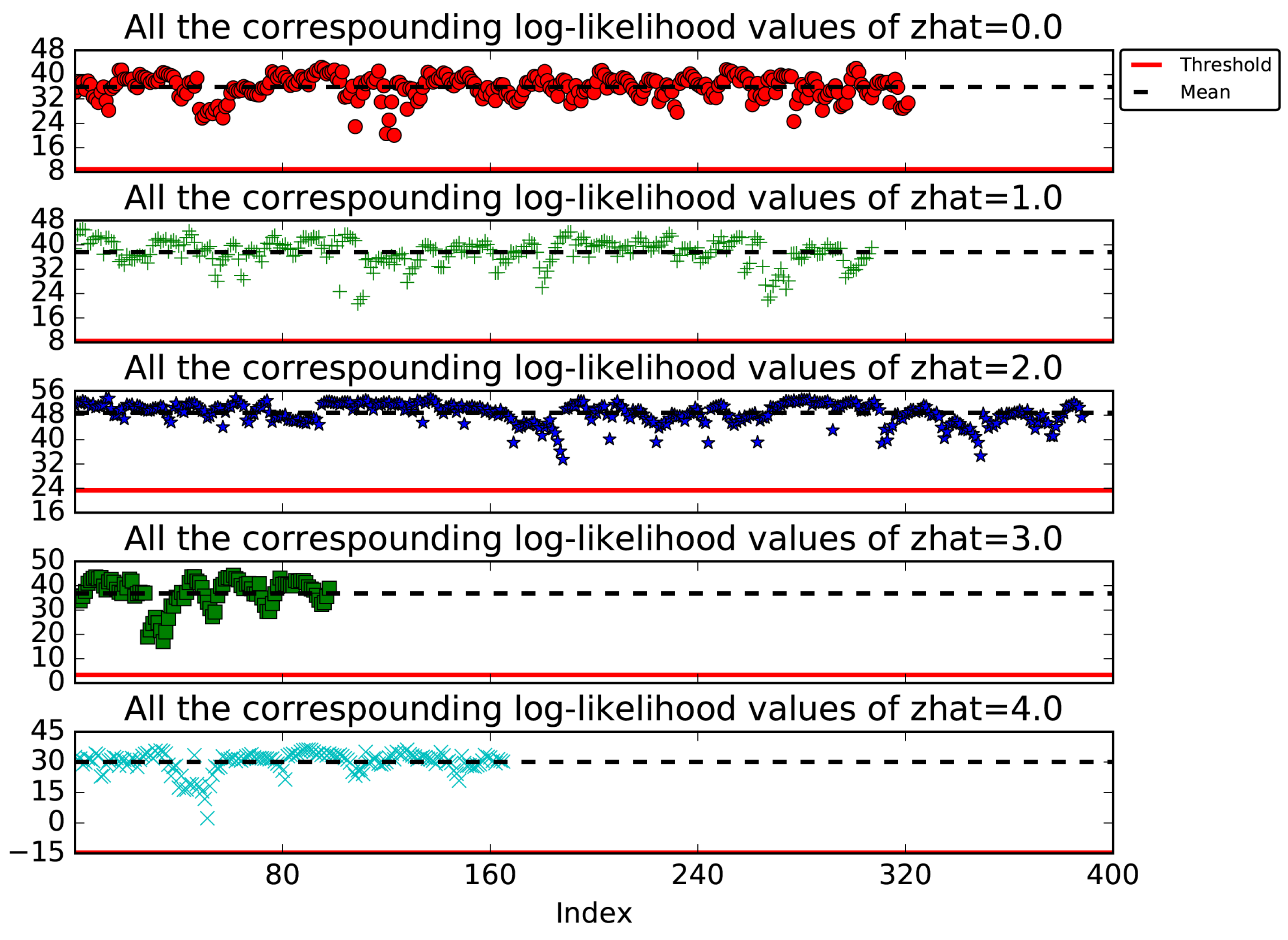
4.3. Hidden-State Estimation of Auto-Regressive Model

For offline construction of the state and log-likelihood pairs, we are interested in the most likely state sequence upon an observation sequence $y_{0:T}$. One might be derived from copulating

The MAP sequence by maximizing the marginal probability at each observation i

$${\widehat{z}}_i=\underset{z_i}{argmax}p\left(z_i\right|y_{0:T}).$$

(21)

We note this combined single-observation estimated sequence might yield unlikely (even 0-probability) sequences. We therefore consider

$${\widehat{z}}_{1:T}=\underset{z_{1:T}}{argmax}p(z_{1:T},y_{0:T}).$$

(22)

where $p(z_{1:T},y_{0:T})$ was computed in Equation (17). Actually, we note the most likely state sequence that the minimum cost path to $z_t$ is equivalent to the minimum cost path to node $z_{t-1}$ plus the cost of a transition from $z_{t-1}$ to $z_t$, and the cost incurred by observation $y_t$.

For convenience, we abbreviate the joint log-likelihood function $\mathcal{L}\left(z_{1:T}\right)\triangleq logp(z_{1:T},y_{0:T})$, and the transition probability ${\pi }_{z_{t-1}}\triangleq z_{t-1}$, then

$${\mathcal{L}}_T\left(z_{1:T}\right)=s_1\left(z_1\right)+\sum _{t=2}^T{s}_t(z_t,{\pi }_{z_{t-1}}),$$

(23)

where

$$\begin{array}{cc}\hfill s_1\left(z_1\right)& =log\left({\pi }_{z_1}p\left(y_1\right|{\theta }_{z_1},y_0)\right),t=1\hfill \\ \hfill s_t(z_t,z_{t-1})& =log\left(p\left(z_t\right|z_{t-1})p\left(y_t\right|{\theta }_{z_t},y_{t-1})\right),t\ge 2\hfill \end{array}$$

(24)

Obviously, ${\mathcal{L}}_t\left(z_{1:t}\right)={\mathcal{L}}_{t-1}\left(z_{1:t-1}\right)+s_t(z_t,z_{t-1})$, and set

$$\begin{array}{cc}\hfill {\upsilon }_t\left(z_t\right)& =\underset{z_{1:t-1}}{max}{\mathcal{L}}_t\left(z_{1:t}\right),z_t\in \{1,2,3,\dots ,K\}\hfill \\ \hfill {\upsilon }_t\left(z_{t-1}\right)& =\underset{z_t}{max}\{{\upsilon }_{t-1}\left(z_t\right)+s_t(z_t,z_{t-1})\},\hfill \end{array}$$

(25)

From the above, the maximizing state sequence is iteratively obtained, for $n\in \{T-1,T-2,\dots ,1\}$

$${\widehat{z}}_T=\underset{z_{t-1}}{argmax}{\upsilon }_n\left(z_{t-1}\right),$$

(26)

Assume that we recorded N sequential data for each skill and the length of sequence $n\in N$ is $T_n$. Thus, we can get a set of the most probable states vector of each skill

$${\mathcal{Z}}^{1:N}=\{{\mathcal{Z}}_{T_1}^1,{\mathcal{Z}}_{T_2}^2,\dots ,{\mathcal{Z}}_{T_N}^N\}.$$

(27)

4.4. Threshold Calculation

With computed the joint probability of the observations and the most probable states for each Skill s, we can concatenate them to compute the threshold of specific state $z=k$ that is $\rho \left(z_k\right)$. Each state consists of its maximum ${\mathcal{L}}_{z_k}^{max}$ and minimum ${\mathcal{L}}_{z_k}^{min}$. We cluster the log-likelihoods with the same state, which represents the clustering data by HMM belonging to the same statistical distribution.

$$\begin{array}{cc}\hfill {\mathcal{L}}_{z_k}^{max}& =\underset{i\in \{1,\dots ,N\}}{max}{\mathcal{L}}_i^n\mathbf{1}(z_k==k),\hfill \\ \hfill {\mathcal{L}}_{z_k}^{min}& =\underset{i\in \{1,\dots ,N\}}{min}{\mathcal{L}}_i^n\mathbf{1}(z_k==k),\hfill \\ \hfill {\mathcal{L}}_{z_k}^{range}& ={\mathcal{L}}_{z_k}^{max}-{\mathcal{L}}_{z_k}^{min},\hfill \end{array}$$

(28)

where the notation $\mathbf{1}\left(\eta \right)$ to represent an indicator random variable is 1 if the event $\eta$ occurs and 0, otherwise. Using Equation (28), we can set the anomaly detection threshold of each active state $z_k$ at any moment according to:

$$\rho \left(z_k\right)={\mathcal{L}}_{z_k}^{min}-\frac{{\mathcal{L}}_{z_k}^{range}}{2}.$$

(29)

In testing implementation, we pre-processed the incoming multimodal data in the same scheme as the training process and then get the most possible state $z_{test}$ by recursively computing the filtered marginals and the corresponding log-likelihood ${\mathcal{L}}_{test}$ using Equations (18) and (19) respectively.

$$z_{test}=\underset{1,\dots ,K}{argmax}\{p(z_t=1|y_{0:t}),\dots ,p(z_t=K|y_{0:t})\}.$$

(30)

Here, this approach detects an anomaly when the log-likelihood is lower than the state-dependent threshold $\rho \left(z_{test}\right)$. This approach also extends to online detection. Given the trained sHDP-VAR-HMM and streaming sensor data, the detector can recursively compute the $z_t$ and ${\mathcal{L}}_t$ at time t, and then perform the comparison; if ${\mathcal{L}}_t<\rho \left(z_{test}\right)$, then anomaly, otherwise nominal.

5. Anomaly Classification

5.1. Problem Formulation

The anomaly classification is triggered once an anomaly is detected. A system can possibly address a wide variety of types of anomalies including low-level hardware anomalies—sensor and actuator noise or breakage—mid-level software contingencies—logic errors or run-time exceptions— or high-level misrepresentations—poor modeling of the robot, the world, their interactions, or external disturbances in the environment [44]). In [43], Park et al. identified both the anomaly class and the cause. In this work, we deal with anomalies caused by external disturbances generated either by intrusive human behavior or resulting from poor modeling or anticipatory ability on the robot side.

We consider the problem of multiclass classification based on multivariate time series, that is, to find a function $f\left(y^n\right)=c^n$ given the $i.i.d$ training data $Y={\left\{y^n\right\}}_{n=1}^N$, $C={\left\{c^n\right\}}_{n=1}^N$, where $y^n=[y_0^n,y_1^n,\dots ,y_{T_n}^n]$ is an observation sequence and $c^n\in \{1,\dots ,c\}$ its corresponding anomaly class. An observation $y_t^n\in {\mathbb{R}}^d$ consists of the same multimodal features as described in Section 3.2 at time step t. Our objective is classification, where given a new test observation sequence $\widehat{y}$, we must predict its corresponding anomaly class $\widehat{c}$. Here, the $\widehat{y}$ is recorded by considering a $window\_size$ around the anomaly moment, and the $\widehat{c}$ is labeled manually during training procedure. We represent each anomaly class by a separate sHDP-VAR-HMM as outlined in Section 3.2; the ${\mathsf{\Theta }}_c$ are the parameters for class c. It would be straightforward to estimate the posterior density of parameters $p\left({\mathsf{\Theta }}_c\right)|Y,C)$ by

$$p\left({\mathsf{\Theta }}_c\right|Y,C)=p\left({\mathsf{\Theta }}_c\right)\prod _{c^n=c}p\left(y^n\right|{\mathsf{\Theta }}_c)p\left(c\right).$$

(31)

That is, each sHDP-VAR-HMM is trained separately and a conditional density $p\left(y\right|c)$ for each class is trained throughout the procedure as defined in Algorithm 1.    

Algorithm 1: Training model for anomaly classification.

5.2. Multiple Classes Anomaly Classifier

As discussed above, we can jointly model N sequences for each class to construct an sHDP-VAR-HMM model. The sequences are used as training and testing samples to evaluate the learned model. The ${\mathsf{\Theta }}_c$ parameters of a specific class model c are estimated using these training sequences. The model assigns a probability to any given testing sequence. In general, good models yield a higher probability score than those outside this class. The probability score can thus be interpreted as a measure of the extent to whether a new sequence is native to the class of interest or not. For our model performance during testing, we evaluate a test sequence $y^{test}=[y_0^{test},y_1^{test},\dots ,y_{T_{test}}^{test}]$ against all the classes and select the class with the largest cumulative log-likelihood (see Equation (18)) as the predicted class $c^{*}$ by

$$c^{*}=\underset{{\mathsf{\Theta }}_c}{argmax}\left(p\left({\mathsf{\Theta }}_c\right|y^{test})\right).$$

(32)

6. Verification

6.1. Experimental Setup

In this section, we describe the kitting experimental setup, external disturbances, data collection, and anomaly detection and classification model parameters.

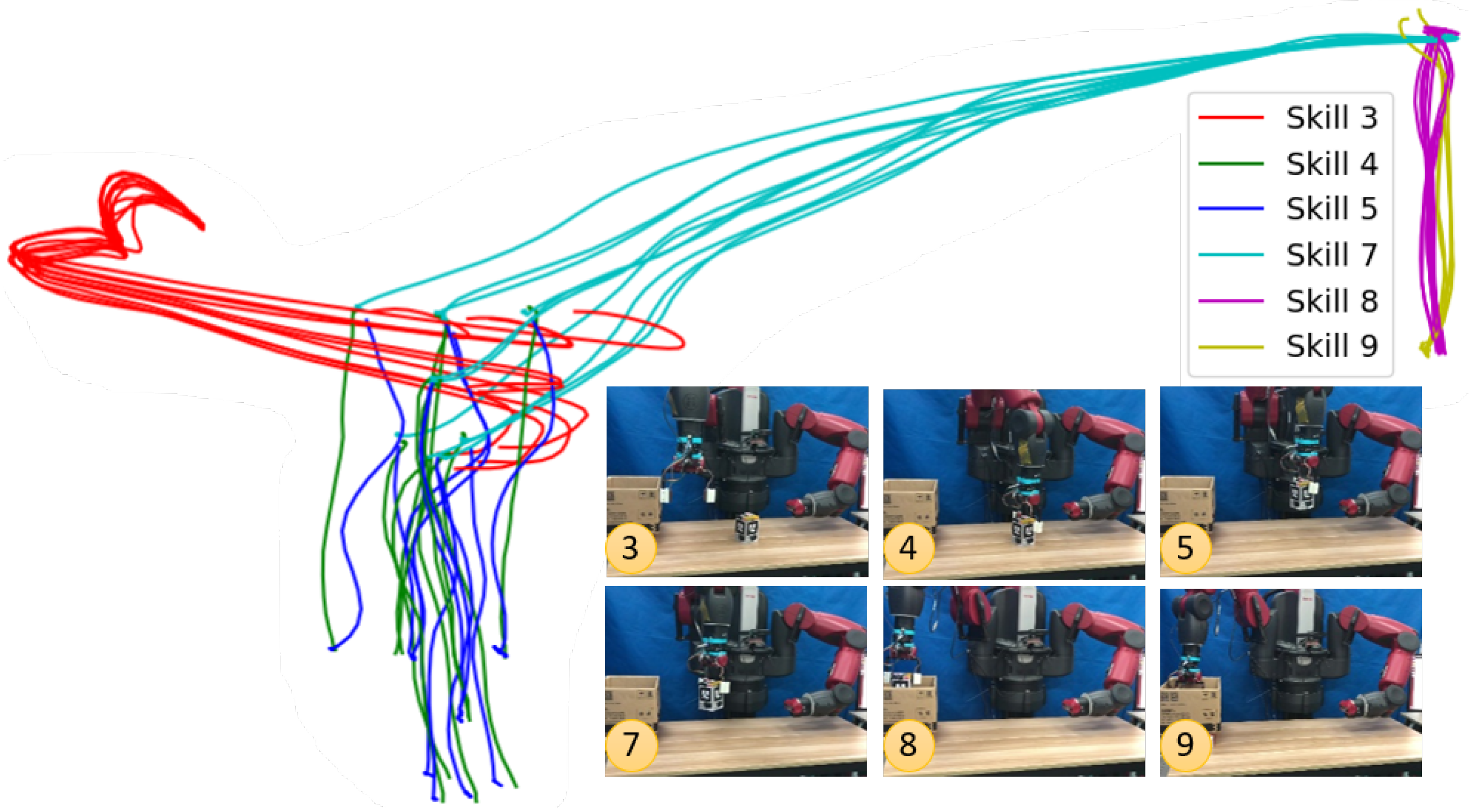
6.1.1. Finite-State Machine Based Kitting Experiment

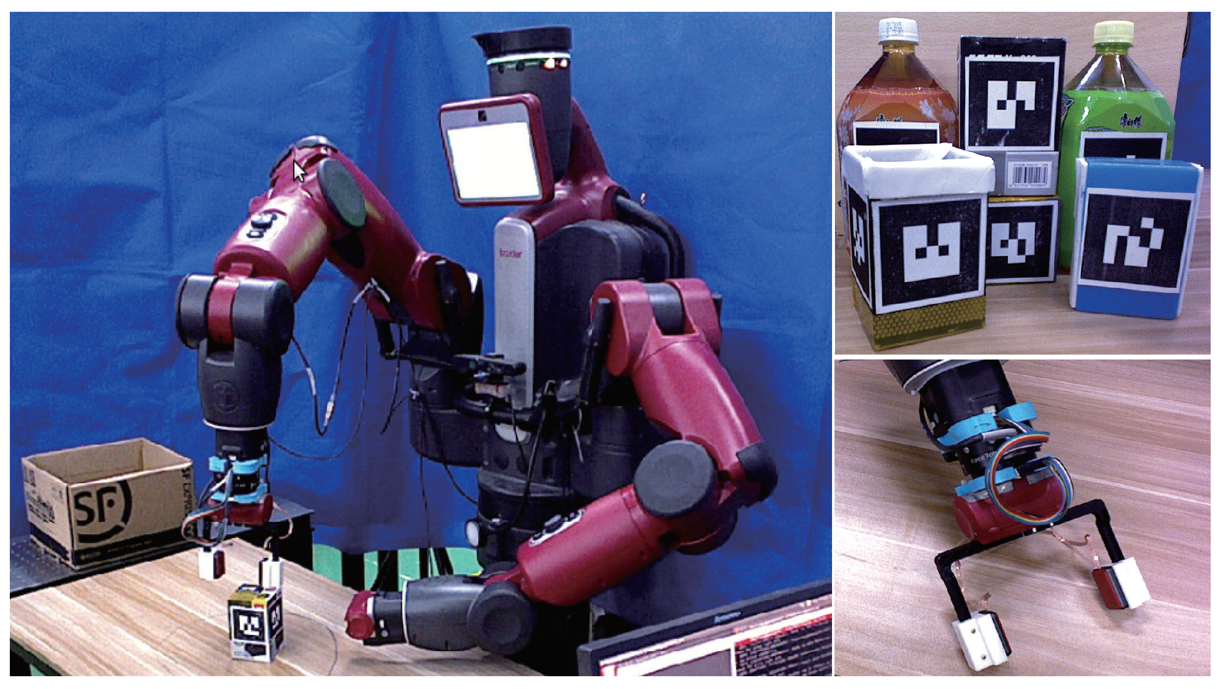
A kitting experiment is set up, where a robot and a human co-worker closely collaborate to place a set of goods in a packaging box. Specifically, a human co-worker is tasked to place a set of 6 objects on the robot’s “collection bin” (located in front of the robot) in a one-at-a-time fashion. The objects may accumulate in a queue in front of the robot. As soon as the first object is on the table, the robot identifies the object and places it in a packaging box located to the right of the robot. Thus, the robot picks an object and transports it towards the box, after which, the robot appropriately places each of the six objects in different parts of the box. The whole implementation is shown in Figure 4. The kitting experiment consists of 6 skills (Skill 3): Home → Pre-pick; (Skill 4): Pre-pick → Pick; (Skill 5): Pick → Pre-pick; (Skill 7): Pre-pick → Pre-place; (Skill 8): Pre-place → Place; (Skill 9): Place → Pre-place) that were effectively modeled by the dynamic movement primitives described in Section 3.1 and the ROS-SMACH (http://www.ros.org/SMACH). One-shot kinesthetic demonstrations were used to train DMP models for each of the skills of the kitting experiment. Please note that a skill’s starting and ending pose can be adapted if necessary, thus providing a flexible and generalizable skill-encoding procedure. The trajectory adaptations however increase the difficulty of assessing the sensory data for both anomaly detection and classification, due to the variability in the data collection even from nominal executions.

6.1.2. The Robot

A Baxter humanoid robot’s right arm is used to pick commonplace objects set before him. The robot is equipped with a 6 DoF Robotiq FT sensor, 2 Baxter-standard electric pinching fingers, as well as Baxter’s left-hand camera. Each finger is further equipped with a multimodal tactile sensor composed of: (i) a 4 × 7 taxel matrix that yields absolute pressure values; (ii) a dynamic sensor which provides a single capacitive reading in millivolts (mV) useful to detect tactile events; and (iii) an IMU and gyroscope [54]. Baxter’s left-hand camera is placed flexibly in a region that can capture objects in the collection bin with a resolution of 1280 × 800 at 1 fps (we are optimizing pose accuracy and lower computational complexity in the system). The use of the left-hand camera facilitated calibration and object tracking accuracy.

6.1.3. Objects

A set of 6 common household objects consisting of box-like shapes and bottles were used in our work. The objects ranged in weight from 0.0308 kg to 1.055 kg and in volume from $3.2\times {10}^{-4}$ m${}^3$ to $1\times {10}^{-3}$ m${}^3$. The object’s surfaces also varied slightly: some heavier objects had sleeker surfaces to incite object slips—we believe not an unreasonable determination as warehouses contain a wide variety of objects—while other objects had rougher surfaces. Across executions, object locations and order were varied to promote generalization.

6.1.4. Visual System

ALVAR tags (http://wiki.ros.org/ar_track_alvar), with 0.06 m sides, were placed around the circumference of the objects for robust visual recognition (ALVAR can handle change in lighting conditions, optical flow-based tracking, and good performance for multitag scenarios) regardless of orientation.

6.1.5. External Disturbances

External disturbances may be introduced into a system for a variety of reasons. We list possible scenarios in which disturbances may occur in real-systems, as shown in Figure 5:

• For collaborative jobs (such as kitting in warehouses; see the description in Section 6.1.1), humans may experience monotony leading to boredom and loss of attention. In such cases, it is possible for a human co-worker to accidentally collide with the robot manipulator or alter the environment in unexpected ways.
• The user may also accidentally collide or unintentionally move packaging objects in ways a robot may not anticipate. Such variations in the world may lead to tool collisions.
• Picked objects may slip from a robot’s gripper if the grasp is not optimal; or if upon motion, inertial forces acting on the object cause slippage that breaks the grasp.
• Object slips may also be caused due to human collisions. Such phenomena depict a chain of anomaly reactions where one anomaly leads to another.
• The robot may also collide with packaging box during kitting.
• Missed grasps (where the robot pinches air) are possible when the target object is moved without the robot noticing.
• Additionally, it is possible to suffer from false positives from the anomaly detector. False positives may occur for numerous reasons: system error, unreachable objects, unfeasible inverse kinematic solutions, unidentifiable objects from the visual system, to name a few.

The seven types of anomalies we just described will be declared more succinctly in the rest of the paper as: Human Collisions (HC), Tool Collisions (TC), Object Slips (OS), Human Collision with Object (HCO), Wall Collision (WC), No Object (NO), and Other (OTHER). In Section 3.2, the introspection methodology is used to model robot skills, followed by a presentation of anomaly detection in Section 4 and anomaly classification in Section 5.

6.2. Dataset Collection

6.2.1. Deducing Anomalies

It is undeniable that bias exists on the side of robot researchers as to which anomalies may exist in the task. In this work, we first attempt to discover likely anomalies in this task by emulating a collaborative kitting task in which the human collaborator experiences tedium and monotony resulting in undesired events that lead to anomalous events.

6.2.2. Human Collaborators

We tasked 5 participants, whose ages range from 23 to 28, to act as a collaborator in the kitting task under the monotonous conditions mentioned in Section 6.1.1. One expert user and four novice users participated in the experiments. Novice users learned from the expert to induce anomalies by observing a round of executions. Each participant performed 1 nominal and 6 anomalous executions by placing the set of six household objects in a one-by-one fashion. For training, when an anomaly occurs, the robot execution is halted and the data stream is labeled with an anomaly class (namely the labels of Section 6.1.5: HC, TC, OS, NO, etc.) for supervised classification during testing. Subsequently, anomalous time stamps are also extracted. In total, we collected a data set with 18 nominal executions and 180 anomalous executions (each anomalous trial has at least one anomaly across the entire task), and 38 failure trails are ignored.

6.2.3. Anomaly Classification Window Considerations

Please note that when an anomaly detection is flagged, we consider a window of time duration $\pm window\_size$ for the subsequent anomaly classification (We use the Redis database for this purpose (https://redis.io/) as rosbags can only be processed offline.). In cases where an anomaly is detected towards the beginning of a skill execution, and the duration of existing data prior to the detection is less than our $window\_size$, in this work, we do not extract data for classification as we deem a minimal presence of signals before and after the detection crucial for the classification. The sensory-motor data collected at this stage allows us to build basic models of the anomalies described in Section 7.1.

6.3. Sensory Pre-Processing

As for our multimodal observation vector, it is comprised of 6 DoF force-torque signals, 6 DoF Cartesian velocity signals (from Baxter’s right-end effector), and 56 DoF tactile signals from both the left and right tactile sensors. Empirical feature extraction is performed on this observation vector to improve classification performance. We now describe how features for each modality at time t were engineered.

Wrench modality: Assume the force and torque sequence is a time-series vector and that each element represents the magnitude of each dimension $(f_x,f_y,f_z,t_x,t_y,t_z)$. We wish to extract structural information from the wrench instead of simply using raw values. In this way, we can find signal patterns that may occur across the different DoFs. To this end, we computed the norm of both the force $n_f$ and the torque $n_t$ as features respectively:

$$n_f=\sqrt{f_x^2+f_y^2+f_z^2},n_t=\sqrt{t_x^2+t_y^2+t_z^2}.$$

(33)

Velocity modality: Similarly, we take the Cartesian linear $(l_x,l_y,l_z)$ and angular $(a_x,a_y,a_z)$ velocities and compute their norm $n_l$ and $n_a$ respectively:

$$n_l=\sqrt{l_x^2+l_y^2+l_z^2},n_a=\sqrt{a_x^2+a_y^2+a_z^2}.$$

(34)

Tactile modality: Due to the computational cost of processing the tactile sensor’s high dimensionality, we empirically tested several features for each tactile sensor, which include the maximum taxel value, the largest five taxel values, the mean of all taxel values, and the standard deviation for all taxel values. It was the standard deviation, which proved to be the most useful feature for anomaly detection and classification. The standard deviation for each tactile sensor $s_l$ and $s_r$ are defined as:

$$s_l=\sqrt{\frac{1}{28}\sum _{i=1}^{28}(l_i-{\mu }_l)},s_r=\sqrt{\frac{1}{28}\sum _{i=1}^{28}(l_i-{\mu }_r)}.$$

(35)

where ${\mu }_l=\frac{1}{28}{\sum }_{i=1}^{28}{l}_i$ and ${\mu }_r=\frac{1}{28}{\sum }_{i=1}^{28}{r}_i$ are the mean of each tactile sensor, respectively. Equations (33)–(35) facilitate the identification of diverging signals during anomalous situations. We empirically concatenate all the valuable features for representing the robot executions both in nominal and anomalous cases. If raw signals are used directly, they result in high false-positive detection rates (FPR) in our experimentation. For instance, when a robot carries objects of varying weights, the F/T signals for such operations vary significantly, making it difficult to use raw values for detection. Hence, a standardization method is used to scale the extracted features through a normalization constant. We end with a feature vector of length 18 as shown below:

$$\begin{array}{cc}\hfill y_t=[& \frac{f_x}{10},\frac{f_y}{10},\frac{f_z}{10},\frac{t_x}{10},\frac{t_y}{10},\frac{t_z}{10},\frac{n_f}{10},\frac{n_t}{0.4},l_x,l_y,l_z,a_x,a_y,a_z,\frac{n_l}{0.4},n_a,\frac{s_l}{250},\frac{s_r}{250}].\hfill \end{array}$$

(36)

Figure 6 illustrates an example of the multimodal signals in a whole nominal experiment with six skills.

Note that all training and testing data are pre-processed in the same manner. We will also use the same pre-processing approach when compared to other baseline approaches.

6.4. Basic Parameter Settings of Each Model

For anomaly detection and classification using the sHDP-VAR-HMM with a first-order auto-regressive Gaussian likelihood, each state k has two parameters to be defined: the regression coefficient matrix $A_k$ and the precision matrix ${\mathrm{\Lambda }}_k$. The conjugate prior is the MNIW, for which four parameters $\nu ,\Delta ,V,M$ are assigned values in a fashion similar to the Motion-Capture-Dataset in [53]. In order to guarantee the prior has a valid mean, the degrees-of-freedom variable is set with $\nu =d+2$ and we set $\Delta$ by constraining the mean or expectation of the covariance matrix $\mathbb{E}\left[{\mathrm{\Lambda }}_k^{-1}\right]$ under the Wishart prior in Equation (11).

$$\mathbb{E}\left[{\mathrm{\Lambda }}_k^{-1}\right]=s_F\sum _{n=1}^N\sum _{t=1}^{T_n}(y_t-\overline{y}){(y_t-\overline{y})}^T.$$

(37)

Assume that we record N sequential data for each skill and the length of sequence $n\in N$ is $T_n$. Thus, we can easily define the parameter $\Delta$ accordingly as

$$\Delta =(\nu -d-1)\mathbb{E}\left[{\mathrm{\Lambda }}_k^{-1}\right].$$

(38)

Specifically, we placed a nominal prior on the mean parameter with mean equal to the empirical mean and expected covariance equal to a scalar $s_F$ times the empirical covariance, here $s_F=1.0$. This setting is motivated by the fact that the covariance is computed from pooling all the data and it tends to overestimate mode-specific covariances. A value slightly less than or equal to 1 of the constants in the scale matrix mitigates the overestimation. Also, setting the prior from the data can move the distribution mass to reasonable parameter space values. The mean matrix M and V are set such that the mass of the MN distribution is centered around stable dynamic matrices while allowing variability in the matrix values (see Section 3.2 for details).

$$\begin{array}{cc}\hfill M& ={\mathbf{0}}_d,\hfill \\ \hfill V& =1.0\ast {\mathbf{I}}_d.\hfill \end{array}$$

(39)

where ${\mathbf{0}}_d$ and ${\mathit{I}}_d$ are the matrix of all zeros and the identity matrix, respectively, each of size $d\times d$. For the concentration parameters, a $Gamma(a,b)$ prior is set on HDP concentration parameters $\alpha$. A $Beta(c,d)$ prior is set on the self-transition parameter $\mu$ and the degree of self-transition bias $\kappa$ is set to 50. We choose a weekly informative setting and choose $a=0.5,b=5,c=1,d=5$. Specifically, the initial transition proportion parameter is set $\mu \sim Beta(1,10)$. The Split-Merge Monte Carlo method sampling parameter maximum iterations is set to 1000. The truncation states number is set to $K=5$ for anomaly detection, and $K=10$ for anomaly classification. Then, the HDP-HMM model of each anomaly class or nominal skill is trained throughout the procedure, as defined in Algorithm 1. Note that, as with pre-processing, we also use the same model parameters in training and testing as well as in other baseline approaches.

7. Results and Analysis

7.1. Anomaly Detection in Kitting Experiment

According to Section 4, the anomaly detector implementation consists of representing multimodal observations through latent states, concatenating the derived log-likelihood values of a latent state, and calculating the anomaly detection threshold.

We first show a visualization of the latent state sequences to illustrate the latent state partitions for nominal demonstrations. Figure 7 illustrates hidden-state partitions for 20 nominal executions for Skill 3 that were carried out with varying speeds and goals. Notice how the non-parametric method yields varying dynamics across executions reflecting statistical variations in the robot motion trajectory due to changes in the desired trajectory completion time and varying goal distances.

Then, latent state log-likelihood values are concatenated, and the corresponding thresholds computed. To this end, we visualized the performance of the proposed method as well as a baseline by assessing the anomaly time reaction of anomaly flags; that is, which algorithm can make a correct detection at a time closer to the ground truth. For training, ten nominal executions were used along with 3-fold cross validation to obtain nominal sHDP-VAR-HMM models for each skill. The other 20 nominal executions were used for testing.

The execution varying threshold for anomaly detection was set according to Equation (29). The results for Skill 3 are visualized in Figure 8. As seen in Figure 7 and Figure 8, latent state $zhat=2$ (the orange state in Figure 7) is the most prominent latent state (the majority of the observations in the skill are ascribed to this state). We now analyze the time sensitivity of our system in detecting anomalies. Anomaly identification sensitivity is intimately connected to threshold setting. We compare the results of our execution varying threshold with a fixed threshold presented in [2]. The comparison is seen in Figure 9. Under nominal situations, both methods have the same robustness in avoiding false positives. In anomalous situations, there are multiple occasions in which our varying threshold yielded better time sensitivity and detection accuracy. From Figure 9, we see that for executions 2 and 4 our varying threshold detector identified anomalies that the fixed threshold method could not. Notice that the distance between the $anomaly\_t\_by\_human$ and the $anomaly\_t\_by\_detector$ is larger for the fixed threshold (recall from Section 6.2 that ground truth time stamps were obtained during training). This improved sensitivity reduces false negatives and helps us flag anomalies at times closer to the ground truth.

Finally,

Table 1. The comparison of anomaly detection performance measures between our proposed method and a baseline method.

Kitting Experiment	Testing Information		Precision		Recall		F1-Score		Accuracy
Movements	Success	Anomalies	GD	HSD	GD	HSD	GD	HSD	GD	HSD
Home → Pre-prick	141	6	1.0	1.0	0.33	0.50	0.50	0.67	0.973	0.980
Pre-prick → Prick	112	23	1.0	1.0	0.78	0.78	0.878	0.88	0.963	0.963
Prick → Pre-prick	83	28	1.0	0.80	0.04	0.31	0.069	0.45	0.757	0.820
Pre-prick → Pre-place	13	70	1.0	0.84	0.54	0.97	0.704	0.90	0.614	0.843
Pre-place → Place	11	6	1.0	0.40	1.0	1.0	1.0	0.57	1.0	0.769
Place → Pre-Place	8	3	0.0	0.0	0.0	0.0	0.0	0.0	0.889	0.889
Across all skills:	368	136	0.98	0.84	0.47	0.76	0.64	0.80	0.861	0.910

shows the anomaly detection performance for our hidden-state detector (HSD) and the baseline gradient-based detector (GD) for the six skills used in the kitting task for 368 nominal executions and 136 anomalous executions. Our results indicate that while the GD system had the HSD resulting in 16.6% better precision, our system had 61.7% better recall. The difference is significant in reducing false negatives and significantly raising the sensitivity of our system. The sensitivity improvement is almost four times bigger than the difference in precision. For this reason, our system reflects an F1 score that is 25.0% larger and an accuracy that is F1 score, and an accuracy that is 5.7% higher, standing at 91.0%.

7.2. Anomaly Classification in a Kitting Experiment

7.2.1. Dataset

The dataset captures sensory-motor signatures of the kitting task under anomalous scenarios as outlined in this paper. A total of 136 anomalous events were recorded in 142 experimental executions across all skills. The proportions for each anomaly class were as follows: TC 15.7%, HC 16.7%, HCO 16.7%, NO 13.0%, OS 16.7%, WC 15.7%, and OTHER 5.6% (see Section 6.1.5 for details).

7.2.2. Anomaly Data Online Recording

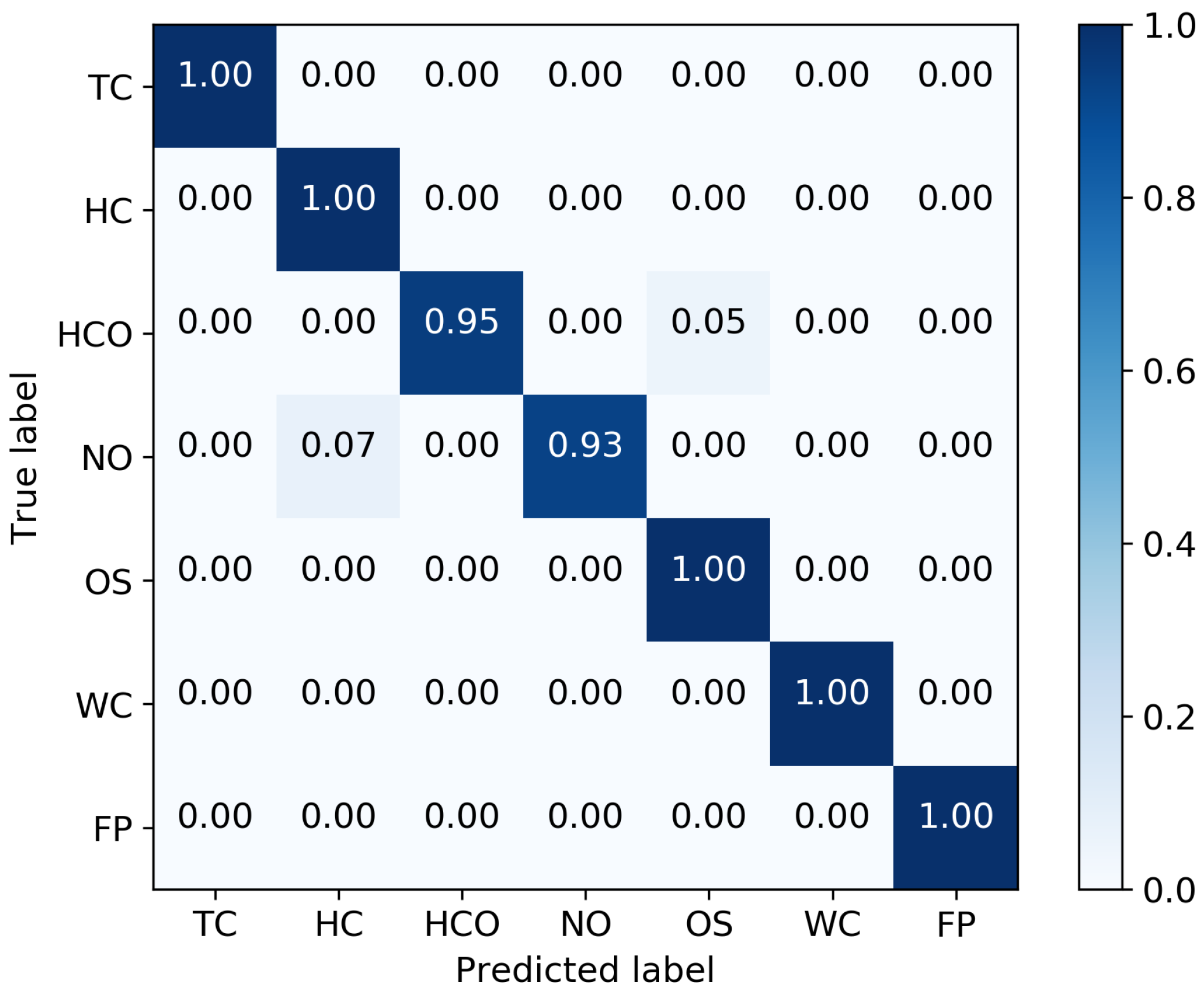
Our system recorded sensory data online. Upon detection of an anomaly, the time step at which the flag occurred is recorded. Then, we record (online) the multimodal signatures (F/T, Cartesian velocity, and tactile signals) before and after the anomaly (also referred to as the sample) according to the time $window\_size$ of Section 6.2. Signals were resampled at 10 Hz to achieve temporal synchronization for all modalities and then further pre-processed as described in Section 6.3. Figure 10 shows an anomaly sample in Skill 7 of TC with $window\_size=2$ s.

7.2.3. Results

To avoid overfitting, we performed 3-fold cross validation for each anomaly type separately. An 18-dimensional feature vector was used as presented in Equation (36). We compare against five baselines consisting of parametric HMMs (with a fixed number of hidden states), various observation models, and various variational inference methods. The training and testing dataset for all the classification methods was the same in this comparison. All methods were trained according to Algorithm 1.

● Parametric HMM Settings: We train 3 differing types of HMMs for each anomaly class. Each HMM uses four different numbers of hidden states $K\in \{3,5,7,10\}$ to train each class. We need to estimate the transition matrix, mean, and covariance parameters. To this end, K-Means++ [55] clusters the data and yields initial estimates. During testing, we evaluate a test sample against all classes and select the class with the largest log-likelihood. The parametric HMMs result summary is presented in

Table 2. The classification accuracy of both classical parametric HMMs and non-parametric HMMs. The best model (observation model and number of hidden states) for each anomaly type is highlighted in blue.

States	Methods	TC	HC	HCO	NO	OS	WC	OTHER	Total Accuracy
3	HMM-Gauss-EM	1.0	0.89	0.89	0.78	0.83	1.0	0.67	0.876
	HMM-Gauss-VB	1.0	0.94	0.95	0.96	0.88	1.0	0.67	0.915
	HMM-AR-VB	1.0	0.89	0.90	0.93	0.94	1.0	0.67	0.929
5	HMM-Gauss-EM	1.0	0.78	0.84	0.79	0.79	1.0	0.67	0.838
	HMM-Gauss-VB	0.94	0.94	0.89	0.86	0.85	1.0	0.67	0.889
	HMM-AR-VB	1.0	0.89	0.95	1.0	0.98	1.0	0.67	0.957
7	HMM-Gauss-EM	1.0	0.83	0.95	0.71	0.77	0.83	0.67	0.826
	HMM-Gauss-VB	1.0	0.83	0.86	0.79	0.82	1.0	0.67	0.863
	HMM-AR-VB	1.0	0.95	1.0	0.93	0.96	1.0	0.67	0.957
10	HMM-Gauss-EM	0.94	0.72	0.85	0.86	0.79	0.94	0.67	0.826
	HMM-Gauss-VB	0.94	0.83	0.95	0.72	0.86	1.0	0.67	0.876
	HMM-AR-VB	0.95	0.83	0.82	0.93	0.92	0.95	0.67	0.889
10	HDP-HMM-Gauss-VB	0.94	0.95	0.95	0.86	0.94	0.90	0.67	0.915
	HDP-HMM-Gauss-moVB	0.88	0.95	0.95	0.93	0.94	0.95	0.83	0.929
	HDP-HMM-AR-VB	0.94	0.84	0.86	0.93	0.96	0.95	0.83	0.915
	HDP-HMM-AR-moVB	1.0	0.95	0.95	0.93	0.98	1.0	1.0	0.971

.

○ HMM-Gauss-EM: A classifier based on a classical HMM with Gaussian observations was trained independently for each anomaly class. The standard Baum-Welch Expectation Maximization algorithm [56] was used to learn the HMM model.

○ HMM-Gauss-VB: A classifier based on classical HMM with Gaussian observation was trained independently for each anomaly class. The standard Variational Bayesian (VB) inference algorithm [57] was used to learn the HMM model.

○ HMM-AR-VB: A classifier based on a classical HMM with first-order auto-regressive Gaussian observations was trained independently for each anomaly class. The standard VB inference algorithm [57] was used to learn the HMM model.

In conclusion, we find that for parametric HMMs (i) the best classification accuracy rate was 95.7% when using 5 to 7 fixed states; (ii) variational inference algorithms outperformed the standard EM algorithm; (iii) the auto-regressive observation model classified better than the Gaussian model due to it is linear conditional nature; (iv) parametric HMMs, in general, are less effective at jointly modeling the dynamics of the robotic task. Therefore, we consider a Bayesian non-parametric version of HMMs with a hierarchical prior, which shares statistical strength across the training samples.

● Non-parametric HMMs Setting: We also train 4 kinds of classifiers based on non-parametric HMMs, independently for each anomaly class. We specify the truncation number of states as K = 10 as explained in Section 3.2. Compared to the parametric HMMs, the actual number of hidden states of each anomaly class is automatically learned from data in non-parametric fashion. The same procedure during testing as described in parametric HMMs. Benefits from the automatic state inference with HDP-HMM, the auto-regressive correlation of the anomaly data, and the effective variational inference techniques. The summary of classification results of non-parametric HMMs are presented in Table 2. Those numbers in blue are denoted the optimal classification accuracy of specific anomaly type across all the methods, respectively.

○ HDP-HMM-Gauss-VB: A classifier based on HDP-HMM with Gaussian observation was trained independently for each anomaly class. The standard VB inference algorithm [32] was used to learn the HDP-HMM model. Similar to the method proposed in [38], instead of the blocked Gibbs sampling algorithm, we learn the model by Variational Bayesian inference.

○ HDP-HMM-Gauss-moVB: A classifier based on HDP-HMM with Gaussian observation was trained independently for each anomaly class. A memorized online variational inference algorithm (moVB) [58] based on scalable adaptation of state complexity is used to learn this HDP-HMM model.

○ HDP-HMM-AR-VB: A classifier based on HDP-HMM with first-order auto-regressive Gaussian observation was trained independently for each anomaly class. The standard VB inference algorithm [32] was used to learn the HDP-HMM model.

○ HDP-HMM-AR-moVB: Finally, our results were evaluated on the HDP-HMM with first-order auto-regressive Gaussian observation for each anomaly class. A memorized online variational inference algorithm (moVB) [58] based on scalable adaptation of state complexity was used to learn this HDP-HMM model.

Given that non-parametric sHDP-VAR-HMM learns the complexity of the model from the data, it produces more accurate models as reflected by the higher classification accuracies shown in Figure 11. The learned number of states for the different anomaly types is shown in Figure 12. Please note that for equivalent parametric HMMs, a tedious model needs to be computed for each class to optimize the state cardinality between types. The diagonal elements represent the number of points for which the predicted label is equal to the true label, while off-diagonal elements are those that are mislabeled by the classifier. It is evident from the confusion matrix that the classification outperforms other baseline methods.

8. Discussion

Comprehensive experimental results showed robust, sensitive, and better-timed anomaly detection and classification for a wide range of anomalous situations in an unstructured co-bot scenario where a human and a robot collaborated to complete kitting tasks. The improved anomaly detector exploits the mapping relationship between latent states and the marginal log-likelihood values from the sHDP-VAR-HMM for monitoring anomalies. The multiclass classifier that is flagged when an anomaly is detected was also tested through the sHDP-VAR-HMM on seven anomalies and six baseline methods. Our evaluations showed that we could not only detect anomalies reliably (overall accuracy of 91.0%) but also classify them precisely (overall accuracy of 97.1%).

With regard to anomaly detection, Table 1 indicated that our proposed detector achieved unexpectedly superior $\mathit{recall}$ measurements compared to the baseline (the gradient-based method of Section 7.1), an improvement of 61.7%. By adjusting the anomaly detection threshold during the task’s progress execution as a function of the maximum and minimum of the log-likelihood of observations for latent states, we gained enhanced sensitivity. Human-centric safety approaches dictate that increased sensitivity is highly desirable in human–robot collaboration tasks to provide higher safety guarantees for a human. Robotic work cells on the other hand may work better with approaches such as the GD (Section 7.1) that was less sensitive but had higher precision. Here the reduction in the false-positive rate may support longer-term autonomy in a work cell. The anomaly detector exhibited not only a better $\mathit{accuracy}$ but also more accurately timed anomaly flags. That is, our anomaly flags occurred closer to the ground truth time. This would be useful. Timeliness may prove a critical role in cases where anomalies are triggered as a chain reaction, i.e., anomalies cause more anomalies. By acquiring more timely detection, we may be able to also provide more timely recovery techniques or even prevention to minimize the possibility of a cascade of anomalies.

With regard to anomaly classification, anomalies usually occur from various sources such as sensing errors, control failures, or environmental changes [59]. If a robot identifies the type, it may be beneficial to prevent or at least recover from the anomalous situation. In our proposed classification method, we trained the sHDP-VAR-HMM model for each anomaly type separately. To address this, Natraj Raman et al. [60] had proposed a signal discriminative HDP-HMM for all classes, albeit with an extra level that is class specific. Thus, an interesting future direction consists of investigating a multilevel sHDP-VAR-HMM for all classes for multiclass classification and the extensions of the observation model by using higher-order auto-regressive Gaussian models.

Development of robot introspection is expected to have a direct impact on a large variety of practical applications, such that can be used to estimate the log-likelihood of failure and prevent failure during robot manipulation tasks. Also, the improvement of safety in the human–robot collaborative environment by assessing the quality of learned internal model for each skill is important, which can speed up the anomaly recovery and/or repair process by providing the detailed skill identification and anomaly monitoring.

There are several limitations in our work. Currently we do not explicitly reduce the influence of outliers occasionally found in the derived log-likelihood values for specific hidden states. The outliers have a significant impact on the calculation of the threshold and our approach needs to address them specifically to avoid their impact. Additionally, we note the fact that our kitting experiment was not conducted under real factory conditions or in a real household daily task. Thus, the verifiability of the work in real-world settings is unclear and further testing in real factory conditions is necessary. The kitting experiment provides a proof of concept and the authors would like to extend their work to actual scenarios through corporate partners.

9. Conclusions

In this paper, we proposed a non-parametric Bayesian method for acquiring a model for a robot skill from raw multimodal sensory data. We are interested in synchronously detecting anomalies and then classifying them. We assume that the skills of a robot in achieving a task can be modeled as a finite-state machine system, where the state is represented with the dynamic movement primitives for generalizing robot discrete movements. The proposed method begins with data recorded by a robot in the execution of a task; we use unsupervised learning techniques to estimate a sHDP-VAR-HMM that can be used both for predicting and explaining the skill of the robot in subsequent executions of the task. Specifically, we introduced a detector that uses a dynamic log-likelihood threshold that varies by latent state for anomaly detection as well as a multiclass classifier, by calculating the cumulative log-likelihood of detected anomalies for anomaly classification. In our evaluations, our proposed anomaly detector outperformed the baseline method for detecting 136 common anomalies and 368 nominal executions with total accuracy of 91.0%. We also had an overall anomaly classification accuracy of 97.1% in anomaly classification for classifying 7 kinds of anomalies from a total of 136 anomalies samples.

References

1. Wu, H.; Lin, H.; Luo, S.; Duan, S.; Guan, Y.; Rojas, J. Recovering from External Disturbances in Online Manipulation through State-Dependent Revertive Recovery Policies. arXiv, 2017; arXiv:1708.00200. [Google Scholar]
2. Luo, S.; Wu, H.; Lin, H.; Duan, S.; Guan, Y.; Juan, R. Robust and Versatile Event Detection through Gradient-Based Scoring of HMM Models. arXiv, 2018; arXiv:1709.07876. [Google Scholar]
3. Ijspeert, A.J.; Nakanishi, J.; Hoffmann, H.; Pastor, P.; Schaal, S. Dynamical movement primitives: Learning attractor models for motor behaviors. Neural Comput. 2013, 25, 328–373. [Google Scholar] [CrossRef] [PubMed]
4. Pastor, P.; Hoffmann, H.; Asfour, T.; Schaal, S. Learning and generalization of motor skills by learning from demonstration. In Proceedings of the 2009 IEEE International Conference on Robotics and Automation (ICRA’09), Kobe, Japan, 12–17 May 2009; pp. 763–768. [Google Scholar]
5. Calinon, S.; Bruno, D.; Caldwell, D.G. A task-parameterized probabilistic model with minimal intervention control. In Proceedings of the 2014 2014 IEEE International Conference on Robotics and Automation (ICRA), Hong Kong, China, 31 May–7 June 2014; pp. 3339–3344. [Google Scholar]
6. Khansari-Zadeh, S.M.; Billard, A. Learning control Lyapunov function to ensure stability of dynamical system-based robot reaching motions. Robot. Auton. Syst. 2014, 62, 752–765. [Google Scholar] [CrossRef] [Green Version]
7. Ronao, C.A.; Cho, S.B. Human activity recognition using smartphone sensors with two-stage continuous hidden Markov models. In Proceedings of the 2014 IEEE 10th International Conference on Natural computation (ICNC), Xiamen, China, 19–21 August 2014; pp. 681–686. [Google Scholar]
8. Goutsu, Y.; Takano, W.; Nakamura, Y. Classification of Multi-class Daily Human Motion using Discriminative Body Parts and Sentence Descriptions. Int. J. Comput. Vis. 2018, 126, 495–514. [Google Scholar] [CrossRef]
9. Wu, H.; Lin, H.; Guan, Y.; Harada, K.; Juan, R. Robot introspection with Bayesian nonparametric vector autoregressive hidden Markov models. In Proceedings of the 2017 IEEE-RAS 17th International Conference on Humanoid Robotics (Humanoids), Birmingham, UK, 15–17 November 2017; pp. 882–888. [Google Scholar]
10. Lemme, A.; Meirovitch, Y.; Khansari-Zadeh, S.M.; Flash, T.; Billard, A.; Steil, J.J. Open-Source Benchmarking for Learned Reaching Motion Generation in Robotics. J. Behav. Robot. 2015, 6, 30–41. [Google Scholar] [CrossRef]
11. Argall, B.D.; Chernova, S.; Veloso, M.; Browning, B. A survey of robot learning from demonstration. Robot. Auton. Syst. 2009, 57, 469–483. [Google Scholar] [CrossRef] [Green Version]
12. Billard, A.; Calinon, S.; Dillmann, R.; Schaal, S. Handbook of Robotics, Chapter 59: Robot Programming by Demonstration. 2007, pp. 131–157. Available online: http://calinon.ch/papers/Billard-handbookOfRobotics.pdf (accessed on 14 March 2019).
13. Niekum, S.; Chitta, S.; Marthi, B.; Osentoski, S.; Barto, A.G. Incremental Semantically Grounded Learning from Demonstration. Robot. Sci. Syst. 2013, 9. [Google Scholar] [CrossRef]
14. Niekum, S.; Osentoski, S.; Konidaris, G.; Chitta, S.; Marthi, B.; Barto, A.G. Learning grounded finite-state representations from unstructured demonstrations. Int. J. Robot. Res. 2015, 34, 131–157. [Google Scholar] [CrossRef]
15. Yu, D.; Deng, L. Automatic Speech Recognition; Springer: Berlin/Heidelberg, Germany, 2016. [Google Scholar]
16. Veenendaal, A.; Daly, E.; Jones, E.; Gang, Z.; Vartak, S.; Patwardhan, R.S. Sensor Tracked Points and HMM Based Classifier for Human Action Recognition. Comput. Sci. Emerg. Res. J. 2016, 5, 4–8. [Google Scholar]
17. Hovland, G.E.; McCarragher, B.J. Hidden Markov models as a process monitor in robotic assembly. Int. J. Robot. Res. 1998, 17, 153–168. [Google Scholar] [CrossRef]
18. Alshraideh, H.; Runger, G. Process monitoring using hidden Markov models. Qual. Reliab. Eng. Int. 2014, 30, 1379–1387. [Google Scholar] [CrossRef]
19. Fox, M.; Ghallab, M.; Infantes, G.; Long, D. Robot introspection through learned hidden markov models. Artif. Intell. 2006, 170, 59–113. [Google Scholar] [CrossRef]
20. Chuk, T.; Chan, A.B.; Shimojo, S.; Hsiao, J. Mind reading: Discovering individual preferences from eye movements using switching hidden Markov models. In Proceedings of the 38th Annual Conference of the Cognitive Science Society (CogSci 2016), Philadelphia, PA, USA, 10–13 August 2016; Cognitive Science Society. 2016. Available online: http://mindmodeling.org/cogsci2016/index.html (accessed on 20 October 2018).
21. Manogaran, G.; Vijayakumar, V.; Varatharajan, R.; Kumar, P.M.; Sundarasekar, R.; Hsu, C.H. Machine learning based big data processing framework for cancer diagnosis using hidden Markov model and GM clustering. Wirel. Pers. Commun. 2017, 102, 2099–2116. [Google Scholar] [CrossRef]
22. Kroemer, O.; Van Hoof, H.; Neumann, G.; Peters, J. Learning to predict phases of manipulation tasks as hidden states. In Proceedings of the 2014 IEEE International Conference on Robotics and Automation (ICRA), Hong Kong, China, 31 May–7 June 2014; pp. 4009–4014. [Google Scholar]
23. Kroemer, O.; Daniel, C.; Neumann, G.; van Hoof, H.; Peters, J. Towards Learning Hierarchical Skills for Multi-Phase Manipulation Tasks. In Proceedings of the 2015 IEEE International Conference on Robotics and Automation (ICRA), Seattle, WA, USA, 26–30 May 2015. [Google Scholar]
24. Teh, Y.W.; Jordan, M.I. Hierarchical Bayesian nonparametric models with applications. In Bayesian Nonparametrics; Cambridge University Press: Cambridge, UK, 2010; Volume 1, pp. 158–207. [Google Scholar]
25. Fox, E.B.; Sudderth, E.B.; Jordan, M.I.; Willsky, A.S. An HDP-HMM for systems with state persistence. In Proceedings of the ACM 25th International Conference on Machine Learning, Helsinki, Finland, 5–9 July 2008; pp. 312–319. [Google Scholar]
26. Bryan, J.D.; Levinson, S.E. Autoregressive Hidden Markov Model and the Speech Signal. Procedia Comput. Sci. 2015, 61, 328–333. [Google Scholar] [CrossRef] [Green Version]
27. Stanculescu, I.; Williams, C.K.; Freer, Y. Autoregressive hidden Markov models for the early detection of neonatal sepsis. IEEE J. Biomed. Health Inform. 2014, 18, 1560–1570. [Google Scholar] [CrossRef]
28. Park, D.; Erickson, Z.; Bhattacharjee, T.; Kemp, C.C. Multimodal execution monitoring for anomaly detection during robot manipulation. In Proceedings of the 2016 IEEE International Conference on Robotics and Automation (ICRA), Stockholm, Sweden, 16–21 May 2016; pp. 407–414. [Google Scholar] [CrossRef]
29. Zhang, A.; Gultekin, S.; Paisley, J. Stochastic variational inference for the HDP-HMM. In Proceedings of the 19th International Conference on Artificial Intelligence and Statistics, Cadiz, Spain, 9–11 May 2016; pp. 800–808. [Google Scholar]
30. Johnson, M.; Willsky, A. Stochastic variational inference for Bayesian time series models. In Proceedings of the International Conference on Machine Learning, Lille, France, 6–11 July 2014; pp. 1854–1862. [Google Scholar]
31. Hughes, M.C.; Fox, E.; Sudderth, E.B. Effective Split-Merge Monte Carlo Methods for Nonparametric Models of Sequential Data. In Advances in Neural Information Processing Systems 25; Pereira, F., Burges, C.J.C., Bottou, L., Weinberger, K.Q., Eds.; Curran Associates, Inc.: Red Hook, NY, USA, 2012; pp. 1295–1303. [Google Scholar]
32. Hughes, M.C.; Sudderth, E.B. Bnpy: Reliable and scalable variational inference for bayesian nonparametric models. In Proceedings of the NIPS Probabilistic Programimming Workshop, Montreal, QC, Canada, 8–13 December 2014. [Google Scholar]
33. Sölch, M.; Bayer, J.; Ludersdorfer, M.; van der Smagt, P. Variational inference for on-line anomaly detection in high-dimensional time series. arXiv, 2016; arXiv:1602.07109. [Google Scholar]
34. Pimentel, M.A.; Clifton, D.A.; Clifton, L.; Tarassenko, L. A review of novelty detection. Signal Process. 2014, 99, 215–249. [Google Scholar] [CrossRef]
35. Milacski, Z.Á.; Ludersdorfer, M.; Lőrincz, A.; Van Der Smagt, P. Robust detection of anomalies via sparse methods. In International Conference on Neural Information Processing; Springer: Cham, Switzerland, 2015; pp. 419–426. [Google Scholar]
36. Rojas, J.; Luo, S.; Zhu, D.; Du, Y.; Lin, H.; Huang, Z.; Kuang, W.; Harada, K. Online Robot Introspection via Wrench-based Action Grammars. arXiv, 2017; arXiv:1702.08695. [Google Scholar]
37. Enrico, D.L.; Tinne, D.L.; Berman, B. HDP-HMM for abnormality detection in robotic assembly. In Proceedings of the NIPS Workshop on Bayesian Nonparametric Models for Reliable Planning and Decision-Making under Uncertainty, Stateline, NV, USA, 3–6 December 2012; pp. 131–157. [Google Scholar]
38. Di Lello, E.; Klotzbucher, M.; De Laet, T.; Bruyninckx, H. Bayesian time-series models for continuous fault detection and recognition in industrial robotic tasks. In Proceedings of the 2013 IEEE/RSJ International Conference on Intelligent Robots and Systems (IROS), Tokyo, Japan, 3–7 November 2013; pp. 5827–5833. [Google Scholar]
39. Hu, D.H.; Zhang, X.X.; Yin, J.; Zheng, V.W.; Yang, Q. Abnormal Activity Recognition Based on HDP-HMM Models. In Proceedings of the Twenty-First International Joint Conference on Artificial Intelligence (IJCAI), Pasadena, CA, USA, 11–17 July 2009; pp. 1715–1720. [Google Scholar]
40. Fu, Y. Human Activity Recognition and Prediction; Springer: Berlin/Heidelberg, Germany, 2016. [Google Scholar]
41. Geurts, P. Pattern extraction for time series classification. In Proceedings of the European Conference on Principles of Data Mining and Knowledge Discovery, Freiburg, Germany, 3–5 September 2001; Springer: Berlin/Heidelberg, Germany, 2001; pp. 115–127. [Google Scholar]
42. Pavlovic, V.; Frey, B.J.; Huang, T.S. Time-series classification using mixed-state dynamic Bayesian networks. In Proceedings of the 1999 IEEE Computer Society Conference on Computer Vision and Pattern Recognition, Fort Collins, CO, USA, 23–25 June 1999; Volume 2, pp. 609–615. [Google Scholar]
43. Park, D.; Kim, H.; Hoshi, Y.; Erickson, Z.; Kapusta, A.; Kemp, C.C. A multimodal execution monitor with anomaly classification for robot-assisted feeding. In Proceedings of the 2016 IEEE International Conference on Robots and Systems (IROS), Vancouver, BC, Canada, 24–28 September 2017. [Google Scholar]
44. Pettersson, O. Execution monitoring in robotics: A survey. Robot. Auton. Syst. 2005, 53, 73–88. [Google Scholar] [CrossRef] [Green Version]
45. Bjäreland, M. Model-Based Execution Monitoring. Linköping Studies in Science and Technology, Dissertation No. 688. 2001. Available online: http://www.ida.liu.se/labs/kplab/people/marbj (accessed on 16 December 2018).
46. Muradore, R.; Fiorini, P. A PLS-based statistical approach for fault detection and isolation of robotic manipulators. IEEE Trans. Ind. Electron. 2012, 59, 3167–3175. [Google Scholar] [CrossRef]
47. Orsenigo, C.; Vercellis, C. Combining discrete SVM and fixed cardinality warping distances for multivariate time series classification. Pattern Recognit. 2010, 43, 3787–3794. [Google Scholar] [CrossRef]
48. Seto, S.; Zhang, W.; Zhou, Y. Multivariate time series classification using dynamic time warping template selection for human activity recognition. In Proceedings of the 2015 IEEE Symposium Series on Computational Intelligence, Cape Town, South Africa, 7–10 December 2015; pp. 1399–1406. [Google Scholar]
49. Karim, F.; Majumdar, S.; Darabi, H.; Harford, S. Multivariate LSTM-FCNs for Time Series Classification. arXiv, 2018; arXiv:1801.04503. [Google Scholar]
50. Pei, W.; Dibeklioğlu, H.; Tax, D.M.; van der Maaten, L. Multivariate time-series classification using the hidden-unit logistic model. IEEE Trans. Neural Netw. Learn. Syst. 2018, 29, 920–931. [Google Scholar] [CrossRef]
51. Baydogan, M.G.; Runger, G. Learning a symbolic representation for multivariate time series classification. Data Min. Knowl. Discov. 2015, 29, 400–422. [Google Scholar] [CrossRef]
52. Schaal, S.; Peters, J.; Nakanishi, J.; Ijspeert, A. Learning movement primitives. In Eleventh International Symposium on Robotics Research; Springer: Berlin/Heidelberg, Germany, 2005; pp. 561–572. [Google Scholar]
53. Hughes, M.C.; Stephenson, W.T.; Sudderth, E. Scalable adaptation of state complexity for nonparametric hidden Markov models. In Proceedings of the 28th International Conference on Neural Information Processing Systems (NIPS’15), Montreal, QC, Canada, 7–12 December 2015; pp. 1198–1206. [Google Scholar]
54. Le, T.H.L.; Maslyczyk, A.; Roberge, J.-P.; Duchaine, V. A highly sensitive multimodal capacitive tactile sensor. In Proceedings of the 2017 IEEE International Conference on Robotics and Automation (ICRA), Singapore, 29 May–3 June 2017; pp. 407–412. [Google Scholar]
55. Arthur, D.; Vassilvitskii, S. K-means++: The advantages of careful seeding. In Proceedings of the 18th Annual ACM-SIAM Symposium on Discrete Algorithms, New Orleans, LA, USA, 7–9 January 2007. [Google Scholar]
56. Welch, L.R. Hidden Markov models and the Baum-Welch algorithm. IEEE Inf. Theory Soc. Newsl. 2003, 53, 10–13. [Google Scholar]
57. McGrory, C.A.; Titterington, D. Variational Bayesian analysis for hidden Markov models. Aust. N. Z. J. Stat. 2009, 51, 227–244. [Google Scholar] [CrossRef]
58. Hughes, M.C.; Sudderth, E. Memoized online variational inference for Dirichlet process mixture models. In Proceedings of the 26th International Conference on Neural Information Processing Systems (NIPS’13), Lake Tahoe, Nevada, 5–10 December 2013; pp. 1133–1141. [Google Scholar]
59. Bicchi, A.; Peshkin, M.A.; Colgate, J.E. Safety for physical human–robot interaction. In Springer Handbook of Robotics; Springer: Berlin/Heidelberg, Germany, 2008; pp. 1335–1348. [Google Scholar]
60. Raman, N.; Maybank, S.J. Action classification using a discriminative multilevel HDP-HMM. Neurocomputing 2015, 154, 149–161. [Google Scholar] [CrossRef] [Green Version]
Figure 1. Manipulation tasks are controlled through a graph-based scheme consisting of nodes and edges. Each node contains three types of modules: (i) motion; (ii) visualization; (iii) and introspection; all of which run in parallel. Motion modules use pose goals provided by the visualization module as well as node-specific skill parameters to generate desirable skills. Introspection modules use node-specific model, parameter, and hyper-parameter settings to continually look for anomalies. If detected, the introspection modules further classify them. A recovery critic then issues a policy for re-enactment or adaptation.
Applsci 09 01072 g001
Figure 2. Autonomous kitting experiment by Baxter robot: The robot is designed to transport 6 markered objects with variable weights and shapes (shown in the top-right subfigure) to a container, where the external anomalies may arise from accidental collisions (human–robot, robot–world, robot/object–world), mis-grasps, object slips, etc. To detect and classify those anomalies, the robot arm is integrated with multimodal sensors (shown in the bottom-right), including internal joint encoders, F/T sensor, tactile sensor, etc.
Applsci 09 01072 g002
Figure 3. (Left) the graphical representation of an HDP-HMM over T time steps. The latent, discrete-valued Markov process z t captures the temporal dependencies in the observations y t . (Right) the graphical model for an HDP-VAR(r)-HMM over T time steps. The latent, discrete-valued Markov process z t dictates the linear dynamical model at time t. For an order r switching VAR process ( r = 1 in this paper), the conditionally linear dynamics are completely determined by previous observations y t 1 . Adapted from [25] by Emily B. Fox.
Applsci 09 01072 g003
Figure 4. A kitting experiment consists of 6 skills (in various colors) that were modeled by DMP, respectively. Objects that need to be packaged are placed by a human collaborator before the robot in a collection bin. The shared workspace affords possibilities for accidental contact and unexpected alteration of the environment. The robot is tasked to pick each one of the objects and place them in the packaging box to its right. The visualization module uses the ALVAR tags to provide a consistent global pose with respect to the base of the robot. Ten nominal executions and one snapshot of each skill are shown.
Applsci 09 01072 g004
Figure 5. Seven representative unexpected anomalies in the kitting experiment (left-to-right): (a) Human Collision (HC), (b) Tool Collision (TC), (c) Object Slip (OS), (d) Human Collision with Object (HCO), (e) Wall Collision (WC), (f) No Object (NO), (g) Other (OTHER).
Applsci 09 01072 g005
Figure 6. Multimodal signals of a nominal experiment with six skills.
Applsci 09 01072 g006
Figure 7. Illustration of the hidden-state representation of Skill 3 when the truncation states number is set to K = 5 . Each row represents the learned hidden-state sequence of a nominal trial. Each color represents a different hidden state. White color indicates a shorter skill duration.
Applsci 09 01072 g007
Figure 8. All the log-likelihood values of individual hidden state of Skill 3 when the truncation states number is set to K = 5 . Each subplot shows the mean value (black dotted line) and the corresponding log-likelihood threshold value (red solid line) in Equation (29).
Applsci 09 01072 g008
Figure 9. The comparison of two anomaly detectors for five robot anomalous executions. Each row represents the same testing execution. Left column: results of our hidden-state-based anomaly detector. Right column: results of the gradient-based anomaly detector [2]. The ground truth ( a n o m a l y _ t _ b y _ h u m a n ) is represented by green dashed lines and the detected anomalies are represented by yellow solid lines.
Applsci 09 01072 g009
Figure 10. A TC sample is shown in the red window of w i n d o w _ s i z e = 2 s.
Applsci 09 01072 g010
Figure 11. Confusion matrix for classification results on kitting experiment dataset with seven anomalies by HDP-HMM-AR-moVB method.
Applsci 09 01072 g011
Figure 12. The number of hidden states being active for different anomaly classes using HDP-HMM-AR-moVB method. An active state is one in which at least one observation is assigned to this state.
Applsci 09 01072 g012