Using Improved Brainstorm Optimization Algorithm for Hardware/Software Partitioning

Abstract

Today, more and more complex tasks are emerging. To finish these tasks within a reasonable time, using the complex embedded system which has multiple processing units is necessary. Hardware/software partitioning is one of the key technologies in designing complex embedded systems, it is usually taken as an optimization problem and be solved with different optimization methods. Among the optimization methods, swarm intelligent (SI) algorithms are easily applied and have the advantages of strong robustness and excellent global search ability. Due to the high complexity of hardware/software partitioning problems, the SI algorithms are ideal methods to solve the problems. In this paper, a new SI algorithm, called brainstorm optimization (BSO), is applied to hardware/software partitioning. In order to improve the performance of the BSO, we analyzed its optimization process when solving the hardware/software partitioning problem and found the disadvantages in terms of the clustering method and the updating strategy. Then we proposed the improved brainstorm optimization (IBSO) which ameliorated the original clustering method by setting the cluster points and improved the updating strategy by decreasing the number of updated individuals in each iteration. Based on the simulation methods which are usually used to evaluate the performance of the hardware/software partitioning algorithms, we generated eight benchmarks which represent tasks with different scales to test the performance of IBSO, BSO, four original heuristic algorithms and two improved BSO. Simulation results show that the IBSO algorithm can achieve the solutions with the highest quality within the shortest running time among these algorithms.

1. Introduction

With the development of semiconductor technology, the application of embedded system is becoming more widely used and it’s architecture is becoming increasingly complex. Because the software processing units (such as CPU, GPU) have the characteristics of short development period, flexibility and easy maintenance, while the hardware processing units (such as ASIC, FPGA) have the characteristics of high efficiency and low power consumption, the development of embedded system needs the hardware and software co-design to satisfy the demands of cost, power, performance and so on.

A task consists of several subtasks, and each subtask may need to be assigned to one type of processing unit. The execution effect of a subtask assigned to the hardware processing unit is different from that assigned to the software processing unit. So the goal of hardware/software partitioning is to get an optimal partitioning scheme to make the system achieve the best performance. Therefore, hardware/software partitioning is the key of the hardware and software co-design.

Hardware/software partitioning is a NP-hard problem [1]. In recent years, many researchers have focused on the study of hardware/software partitioning algorithms. In general, the algorithms applied to hardware/software partitioning can be divided into two categories. One is the accurate algorithms, the other is the heuristic algorithms. Accurate algorithms mainly include dynamic programming (DP) [2,3], integer linear programming (ILP) [4], branch and bound (B&B) [5] and so on. The advantage of accurate algorithms is that it can precisely find the absolute optimal solution of the hardware/software partitioning problem. When it comes to large-scale instances of the problem, the execution of accurate algorithms becomes complicated and time-consuming. Therefore, heuristic algorithms are utilized to solve hardware/software partitioning problem increasingly.

Swarm intelligence (SI) is a discipline inspired by collective behaviors of biological species/systems and consists of many different algorithms. The SI algorithms have the advantages of excellent global search ability and strong robustness. They are suitable for solving complex problems because their optimization process can be seen as a black box [6]. The common SI algorithms include particle swarm optimization (PSO) [7], artificial bee colony (ABC) [8], artificial fish school algorithm (ASFA) [9], ant colony algorithm (ACO) [10], shuffled frog leaping algorithm (SFLA) [11] and so on. In recent years, these algorithms are successfully applied in different areas to solve the complex optimization problems. For example, Fong et al. used the PSO in feature selection [12], Hashim et al. applied the the ABC to optimize the wireless sensor network [13], Dai et al. solved the path-planning problem based on the ACO [14], Qin et al. solved the vehicle routing problem with the ASFA [15], and in our previous work, we designed a local dimming algorithm based on the SFLA [16]. In the hardware/software partitioning area, some SI algorithms were also applied and achieved good performance [17,18,19]. When applying SI to hardware/software partitioning, there are two metrics of interest: the quality of the obtained solutions and the execution time of the algorithms. Therefore, the two metrics are usually used to evaluate the performance of the algorithms.

Brainstorm optimization (BSO)is a young and promising SI algorithm proposed by Shi in 2011 [20]. It was proposed based on the collective behavior of human being, that is, the brainstorming process [21]. After the algorithm was proposed, it was applied in many areas, such as finding the optimal location and setting of devices in electric power systems [22], receding horizon control for multiple UAV formation flight [23], designing the wireless sensor networks [24], and solving equation systems [25]. To improve the performance of BSO, a series of variants were proposed. Zhan et al. proposed a simple grouping method to accelerate the algorithm [26], Zhou et al. proposed the modified step-size to improve the search ability of BSO [27], Yang and Shi used the chaotic operation to improve the individual generation strategy [28], Yang et al. utilied the incorporation of inter-and intra-cluster discussions to balance the global and local searching [29]. There are also some hybrid algorithms. For example, Jia et al. hybridized BSO with simulated annealing algorithm [30], Krishnanand et al. hybridized BSO with the teaching-learning-based algorithm [31]. Because BSO performed well in many applications, it is applied to solve the hardware/software problem in this paper. In most of previous researches, BSO was usually applied to solve continuous optimization problems, but the hardware/software partitioning problem is a discrete optimization problem. Therefore, when the BSO is utilized to solve hardware/software partitioning problem, it has the shortage of premature convergence which will directly affect the quality of solutions. At the same time, the algorithm efficiency should be further improved.

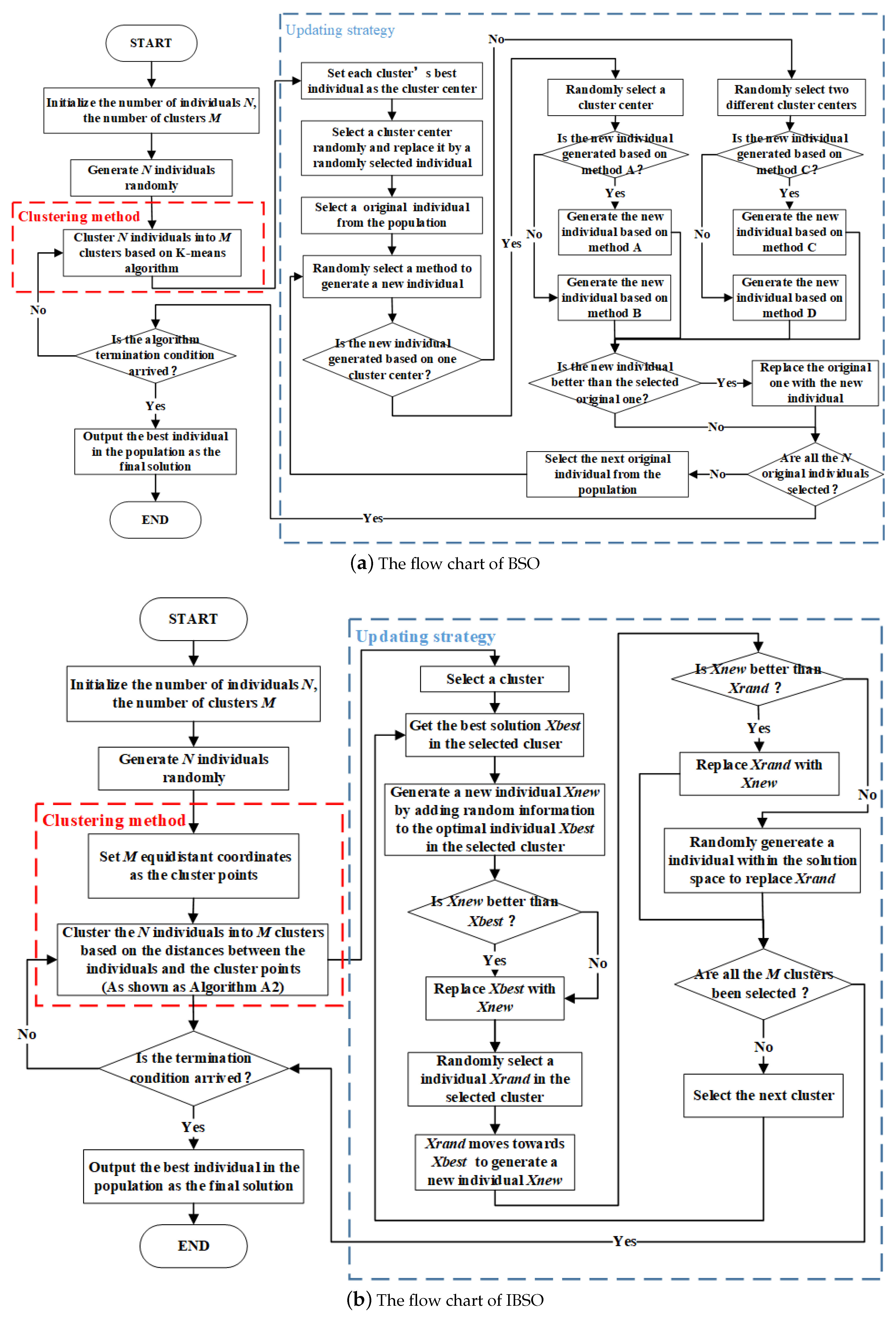
From what has been discussed above, this paper applies the BSO algorithm to hardware/software partitioning and improves its clustering method and updating strategy to generate the improved brainstorm optimization (IBSO) algorithm. Experimental results show that the IBSO algorithm performs well on hardware/ software partitioning.

The rest of the paper is organized as follows. In Section 2, the related knowledge of hardware/ software partitioning problem is described. Section 3 describes the process of BSO algorithm applied to hardware/software partitioning. In Section 4, IBSO algorithm is proposed. Finally, the empirical results and conclusion are elaborated in Section 5 and Section 6 respectively.

2. The Mathematical Model of Hardware/Software Partitioning

The problem of hardware/software partitioning can be expressed as $G=<V,E>$. $V=\{V_1,V_2,\dots ,V_L\}$ is a task which has many subtask nodes, where L is the number of subtask nodes and $V_i$ is the i-th subtask node. $E=\left\{(V_i,V_j)\right|V_i,V_j\in V\}$ represents data dependencies or control process between subtask nodes. A subtask node can be expressed as

$$V_i=<V_{type}\left(i\right),T_s\left(i\right),T_h\left(i\right),C(i,j),A_h\left(i\right),\dots >,$$

(1)

where $V_{type}\left(i\right)=\{0,1\}$ represents the subtask assignment method, $V_{type}\left(i\right)=0$ means the subtask is assigned to software processing unit while $V_{type}\left(i\right)=1$ means the subtask is assigned to hardware processing unit. $T_s$ represents the execution time when the subtask is assigned to software processing unit and $T_h$ represents the execution time when the subtask is assigned to the hardware processing unit. $C(i,j)$ represents the communication time between $V_i$ and $V_j$ when there is dependency between them. $A_h\left(i\right)$ is the required hardware area when the subtask is assigned to hardware processing unit. Compared with hardware processing unit, the required area of software processing unit is much less. So the required area of software processing unit is ignored. In this paper, the total required area of processing units is taken as the constraint, and the time required for the system to complete the task (the completion time of the whole task) is taken as the optimization objective. The mathematical description is given in (2).

$$\begin{array}{c}\min :\hfill \\ T\left(V\right)=max\left\{TE\left(V_i\right)\right|\forall i\in \{1,2,\dots ,L\}\}\hfill \\ \mathrm{subject}\mathrm{to}:\hfill \\ A=\sum _{i=1}^L{A}_h\times V_{type}\left(i\right)\le AreaLimit,\hfill \end{array}$$

(2)

where $T\left(V\right)$ denotes the completion time of the whole task. $TE\left(V_i\right)$ denotes the completion time of the ith path of the task. A denotes the total required area of processing units and $AreaLimit$ is the constraint value.

The solution space of hardware/software partitioning problem can be represented by a L-dimensional discrete space ${\{0,1\}}^L$ , where L is the number of subtask nodes. A solution can be represented by a L-dimensional vector $x_k$ in this space, $x_k=[x_k^1,x_k^2,\dots ,x_k^i,\dots ,x_k^L]$, where $x_k^i=0$ represents the i-th subtask is assigned to software processing unit, while $x_k^i=1$ represents the i-th subtask is assigned to hardware processing unit. For example, a solution of hareware/software partitioning $[1,0,1,1,\dots ]$ means that the first, the third and the fourth subtasks are assigned to the hardware processing unit, and the second subtask is assigned to the software processing unit.

3. Hardware/Software Partitioning Based on BSO Algorithm

3.1. BSO Algorithm

As a novel SI algorithm, BSO is inspired by human beings’ brainstorming process. In the brainstorming process, there are three kinds of roles, a facilitator, a group of people and several clients [20]. The facilitator is responsible for encouraging people to provide ideas as diverse as possible, so that the good ideas can be picked out with higher possibility. The group of people act as the role of providing ideas as diverse as possible. They have enough knowledge about the problem to be solved. Clients act as the owners of the problem. They can evaluate these ideas and select the best one after each iteration.

3.2. The Application of the BSO Algorithm in Hardware/Software Partitioning

In this paper, the BSO algorithm proposed in [20] is applied to solve the problem of hardware/software partitioning. Its pseudo-code is shown in Algorithm 1, where p_replace, p_one, p_one_center, p_two_center are thresholds between 0 and 1.

Algorithm 1. Brainstorm optimization (BSO) applied to hardware/software partitioning.

1 Visual_num = N; Cluster_num = M; /*Initializing the number of individuals and the number of clusters*/

2 Init_visuals(); /*Generating N feasible solutions randomly*/

3 While the termination condition is not arrived

3.1 Cluster(); /*Clustering N individuals into M clusters*/

3.2 Fit_calculate(); /*Calculating the fitness value of each individual*/

3.3 Set_centers(); /*Setting the individual with the best fitness value in each cluster as the center of the cluster*/

3.4 If (random(0,1) < p_replace)

Substitute_center(); /*Selecting a cluster center randomly and replace it by a randomly selected individual*/

End If

3.5 For (j = 1 to Visual_num)

If (random(0,1) < p_one)

Select_one_cluster(); /*Selecting a cluster randomly*/

If (random(0,1) < p_one_center)

New_individual = Create_individual_A(); /*Generating a new individual by method A. Method A is adding random information to the center of the selected cluster to generate a new individual*/

Else

New_individual = Create_individual_B(); /*Generating a new individual by method B. Method B is adding random information to a randomly selected individual in the selected cluster to generate a new individual*/

End If

Else

Select_two_cluster(); /*Selecting two different clusters randomly*/

If (random(0,1) < p_two_center)

New_individual = Create_individual_C(); /*Generating a new individual by method C. Method C is adding random information to the combination of the two selected cluster centers to generate a new individual.*/

Else

New_individual = Create_individual_D(); /*Generating a new individual by method D. Method D is adding random information to the combination of two randomly selected individuals in the selected clusters to generate a new individual.*/

End If

End If

Fit_new = Fit_calculate(New_individual); /*Calculating the fitness value of the new individual*/

If (Is_valid(New_individual)&&Fit_new < Fit_old) /*If the new individual meets the constraint and its fitness value is less than the original one*/

Substitute_individual(); /*Replacing the old individual by the new individual*/

Else

Keep_individual(); /*The old individual will be retained*/

End If

End for

Current_Iteration = Current_Iteration+1;

End while

4 Output (solution); /*Outputting the optimal solution*/

It can be seen from Algorithm 1 that the BSO algorithm mainly contains two steps in each iteration, clustering and updating. In the step of clustering, N individuals are clustered into M clusters based on the K-means algorithm and the center of each cluster is replaced by the individual with the best fitness value in the cluster. In the step of updating, individuals are updated successively. There are four methods to generate new individuals.

(1)

Selecting one cluster randomly, then adding random information to the center of cluster;

(2)

Selecting one cluster randomly, then adding random information to a individual which is randomly selected from the cluster;

(3)

Selecting two clusters randomly, then adding random information to the combination of the centers of the two clusters;

(4)

Selecting two clusters randomly, then adding random information to the combination of two individuals which are randomly selected from the two clusters.

When an individual is being updated, it should select a method to generate a new individual according to predefined probability and determine whether to replace the original individual with the new individual based on their fitness values. The random information $inf$ is calculated as follows:

$$inf=\xi \ast n(\mu ,\sigma ),$$

(3)

where $n(\mu ,\sigma )$ is a Gaussian function whose mean is $\mu$ and variance is $\sigma$, $\xi$ is a coefficient which weights the contribution of the Gaussian random value [32], and $\xi$ can be calculated as follows:

$$\xi =logsig\left(\right(0.5\ast MaxIter-CurIter)/k)\ast rand(0,1),$$

(4)

where $MaxIter$ is the maximum number of iterations. $CurIter$ is the current number of iterations. k is the slope of $logsig\left(\right)$ function, and $rand(0,1)$ is a random value between 0 and 1.

4. Hardware/Software Partitioning Based on IBSO Algorithm

4.1. Analysis of BSO Algorithm

The problem of hardware/software partitioning is a discrete optimization problem and its solution is an L-dimensional vector consisting 0 and 1. Unlike continuous optimization problem, the number of feasible solutions in the solution space of discrete optimization problem is finite. For example, if there are l nodes in a hardware/software partitioning problem, the maximum number of feasible solutions is $2^l$. In previous studies, BSO was usually applied to the continuous optimization problem. But when it comes to the hardware/software partitioning, there are some disadvantages in the clustering method and the updating strategy, which cause the disadvantages of premature convergence, inefficiency and so on.

4.1.1. Clustering Method

The original BSO algorithm uses a K-means algorithm as the clustering method and the numbers of individuals in each cluster may be different. When the clustering process is completed, the optimal individual in each cluster will be taken as the new cluster center and it will be utilized to guide the updating of the individuals. But this clustering method may lead individuals to gather in the same area and cause the algorithm to fall into a local optimum. Figure 1 is an example.

As shown in Figure 1a, it is assumed that all feasible solutions are distributed in three regions: region 1, region 2 and region 3. Suppose there are nine randomly generated individuals, where $x_1,x_2,x_3$ are distributed in region 1, $x_4,x_5,x_6$ are distributed in region 2, $x_7,x_8,x_9$ are distributed in region 3, and $x_7,x_8,x_9$ are the three best individuals in the population. When clustering begins, based on the k-means algorithm, the clustering result is shown in Figure 1b where the cluster 1 includes $x_1,x_2,x_3,x_7$, the cluster 2 includes $x_4,x_5,x_6,x_8$ and the cluster 3 includes $x_9$. Since $x_7,x_8,x_9$ are the best solutions in their own clusters, they will be set as the centers after clustering. Then the individuals begin to update. According to the updating rules, the search direction of individuals will be guided by the cluster centers. In this case, as shown in Figure 1b, the existing individuals will move towards the position of $x_7,x_8,x_9$ which will cause most of the individuals gather to region 3 and the global searching cannot be performed. So the algorithm is easy to fall into local optimum.

4.1.2. Updating Strategy

In the updating process, every individual in the population will try to search for a new individual to update itself. The new individual may be generated by adding random information to a cluster center or to the combination of two cluster centers. However, due to the solution of hardware/software partitioning problem is a vector consisting of 0 and 1, there is a great probability to generate the same or similar new individuals based on the aforementioned updating strategy. If all or most individuals in the population are replaced by the new generated individuals in each iteration, it will be difficult to keep the population diversity as the number of iterations increasing. An example is shown in Figure 2.

Suppose that there are five individuals in a cluster. The original individuals are shown in Figure 2a, and the $Ind5$ is the cluster center. The new individuals might appear as Figure 2b if they are generated by the way of adding random information to the cluster center ($Ind5$). It can be seen that individuals in the cluster will be the same or close. Therefore, if individuals are updated by the original updating strategy, it will affect the diversity of the population. When most individuals in the population are similar, the algorithm is easy to fall into a local optimum, so that the premature convergence phenomenon appears. In addition, if the population diversity cannot be kept, the number of invalid searches will increase. For example, if two new individuals Xn1 and Xn2 are separately searched by two similar individuals X1 and X2 in the current population, the generated individuals Xn1 and Xn2 may be similar or even the same, which means one of the searches may be invalid. With a lot of invalid searches, the efficiency of the algorithm will be reduced. On the other hand, BSO updates all the individuals in the current population in one iteration, that is to say, if the number of individuals is N, updating the individuals needs at least N searches. Compared with updating a small number of individuals in one iteration, the updating strategy of BSO obviously requires more time.

4.2. IBSO Algorithm

In view of the problems above, this paper aims to improve the algorithm from the aspects of clustering method and updating strategy.

4.2.1. Improved Clustering Method

In terms of the clustering method, suppose that there are N individuals to be clustered into M clusters. Firstly, setting M equidistant coordinates in the solution space which can be expressed as $C=\{c_1,c_2,\dots ,c_i,\dots ,c_M\}$, where $c_i$ is an L-dimensional vector, and L is the dimension of the solution. The equidistant coordinates are called cluster points in this paper and $c_i$ is the cluster point of the i-th cluster. Then all individuals are sorted according to their fitness values. Finally, clustering the sorted individuals into the cluster whose cluster point is nearest to them. The Manhattan distance is used as the distance between individuals and cluster points. The $Di{s}_{j,k}$ between individual $x_j$ and cluster point $c_k$ can be calculated by [33]:

$$Di{s}_{j,k}=\sum _{i=1}^L|x_j\left(i\right)-c_k\left(i\right)|,$$

(5)

where $x_j\left(i\right)$ and $c_k\left(i\right)$ are the i-th dimension of $x_j$ and $c_k$ respectively.

In addition, the number of individuals in each cluster must be same. So when the number of individuals in a cluster reaches $N/M$, this cluster is saturated. In this case, the individuals which are not clustered should be clustered to other unsaturated clusters whose cluster points are nearest to them. The pseudo-code of the improved clustering method is shown in Algorithm 2.

Algorithm 2. Improved clustering method

1 Init_points(); /*Initiating M equidistant coordinates as the cluster points*/

2 For (j = 1 to N)

2.1 For (k = 1 to M)

If (!Is_cluster_saturated(k)) /*If the kth cluster is not saturated*/

$Di{s}_{j,k}$ = calculate_distance_with_points(j); /*Calculating distance $Di{s}_{j,k}$ between $x_j$ and $c_k$*/

If (Is_shortest($Di{s}_{j,k}$)) /*If the distance between individual $x_j$ and cluster point $c_k$ is shorter than that between $x_j$ and other cluster points of unsaturated clusters*/

Cluster_number_of ($x_j$) = k; /*Clustering individual $x_j$ into cluster k*/

End If

End If

End for

End for

If the individuals in Figure 1a are clustered by the improved clustering method, the clustering result is shown in Figure 3. It can be seen that individuals in the same region are clustered into the same cluster, which will effectively avoid individuals gathering into a local region in the updating process.

4.2.2. Improved Updating Strategy

In terms of the updating strategy, in one iteration, different from the original algorithm which updates all individuals in the population, the improved algorithm only updates the optimal individual and a random selected individual in each cluster. In addition, in some SI algorithms such as PSO [7], ABC [8] and SFLA [11], an individual updates itself by moving towards other individuals which have better quality. This updating strategy is beneficial for obtaining high quality solutions. Therefore, we introduce this strategy to update the individuals in IBSO. Firstly, updating the optimal individual in the cluster. The optimal individual adds random information to generate a new individual. If the new individual is superior to the original one, replacing the original individual with the new individual. Then, randomly select an individual in the cluster and update it. The selected individual will generate a new individual by moving towards the cluster’s best individual. If the new individual is superior to the original one, replacing the original individual with the new individual. Otherwise, generating an individual randomly in the solution space to replace the original one. The pseudo-code of the improved updating strategy is shown in Algorithm 3 and the calculation of $\xi$ is the same as (4).

It can be seen from Algorithm 3, in one iteration, the improved updating strategy does not update all individuals in the population, it only updates two individuals in each cluster(the best individual and a randomly selected individuals in the cluster), which will reduce the running time of one iteration. The updating of the optimal individual uses the method of adding random information to it. It is advantageous to the optimal individual to jump from the local region. The updating of the randomly selected individual uses the method of moving random length towards the optimal individual, which not only guarantees the difference between the randomly selected individual and the optimal individual, but also helps the randomly selected individual effectively search for better individuals. In addition, some individuals will be updated by the randomly generated individuals, which will better keep the population diversity. Based on the improved updating strategy, individuals in Figure 2a will be updated to new individuals as show in Figure 4. Where the 5th individual is the optimal individual and the first individual is the randomly selected individual.

Algorithm 3. Improved updating strategy

1 For (k = 1 to M)

1.2 $x_{new}=x_{best}^k+inf$; /*Adding random information to the optimal individual $x_{best}^k$ in the kth cluster to generate a new individual $x_{new}$*/

1.3 Fit_new = Fit_calculate($x_{new}$);

1.4 If (Is_valid($x_{new}$)&&Fit_new < Fit_old)

$x_{best}^k=x_{new}$; /*Replacing $x_{best}^k$ with $x_{new}$ if the fitness value(Fit_new) of $x_{new}$ is better than the fitness value(Fit_old) of $x_{best}^k$*/

End If

1.5 $x_{rand}^k=get\_random\_individual\left(k\right);$ /*Randomly selecting an individual $x_{rand}^k$ from the kth cluster*/

1.6 $x_{new}=x_{rand}^k+\xi \ast (x_{best}^k-x_{rand}^k)$; /*Individual $x_{rand}^k$ moves random length towards the optimal individual $x_{best}^k$ in the kth cluster to generate a new individual $x_{new}$*/

1.7 Fit_new = Fit_calculate($x_{new}$);

1.8 If (Is_valid($x_{new}$)&&Fit_new<Fit_old)

$x_{rand}^k=x_{new}$; /*Replacing $x_{rand}^k$ with $x_{new}$ if the fitness value(Fit_new) of $x_{new}$ is better than the fitness value(Fit_old) of $x_{rand}^k$*/

Else do

$x_{new}=random\left(x\right);$ /*Randomly generating a valid individual $x_{new}$ to replace the original individual $x_{rand}^k$ */

while (!Is_valid($x_{new}$));

End If

End If

End for

It can be seen from Figure 4 that by using the improved updating strategy, the population diversity is better kept.

With the improved clustering method and updating strategy, IBSO can successfully avoid the premature convergence and achieve a higher efficiency. The flow charts of BSO and IBSO are shown in Figure 5.

5. Experiments and Discussion

5.1. Experimental Setup

In this paper, we use task graphs for free (TGFF) tool to generate the experimental data. The TGFF tool is a pseudo random task graph generator, it creates problem instances for use in allocation and scheduling research [34]. In the research field of hardware/software partitioning, the TGFF tool is widely used to generate the task graphs to test the performance of Algorithms [19,35,36]. A task graph represents a set of subtask nodes to be partitioned, each node includes the parameters of software execution time, hardware execution time and hardware area, and there is parameter of communication time between two subtask nodes. According to the related studies, these parameters are randomly generated by the TGFF tool within their respective intervals(the intervals of software execution time, hardware execution time, hardware area, and communication time were (800 ms, 2000 ms), (200 ms, 1200 ms), (100 units, 400 units) and (40 ms, 100 ms) respectively). In our experiments, eight different benchmarks were generated from 50 to 1000 nodes. The completion time of the whole task $T\left(V\right)$ was taken as the optimization objective and the required hardware area was taken as the constraint (as shown as Equation (2)). The constraints values $AreaLimit$ of eight benchmarks are shown in

Table 1. The constraint values of eight different benchmarks.

Number	Nodes	AreaLimit (Units)
1	50	6407
2	100	12,181
3	150	18,673
4	200	24,881
5	300	36,844
6	500	62,132
7	700	87,162
8	1000	122,768

.

5.2. Comparison between IBSO and BSO

In this paper, the IBSO algorithm was compared with the BSO algorithm firstly. To compare the search ability of the two algorithms, they were applied to solve the benchmarks with 500 subtask nodes and 1000 subtask nodes. The parameter setting of the two algorithms is shown in

Table 2. Parameter setting of the brainstorm optimization (BSO) and the improved BSO (IBSO).

BSO	IBSO
Populations: 20	Populations: 20
Clusters: 4	Clusters: 4
K: 100	K: 100

and the algorithms were terminated when the number of successive invalid iterations arrived at 150 (the iteration which cannot find a better solution is called invalid iteration in this paper) or the number of iterations arrived at 1000. Based on the $T\left(V\right)$ of the optimal solution obtained in each iteration, we can get the descending curves of the algorithms, which can reflect the search process of the algorithms. Figure 6 shows the descending curves of IBSO and BSO when applied to benchmarks with 500 subtask nodes and 1000 subtask nodes.

It can be seen from Figure 6 that the BSO algorithm terminates after a few iterations and the final solution of the BSO algorithm is poor. In other words, after a few iterations, the BSO is unable to find better solutions although the quality of the current obtained solutions was poor, after 150 successive invalid iterations, the algorithm is terminated and output a poor quality solution. It illustrates that the BSO algorithm was prone to falling into local optimum and premature convergence. When BSO was applied to hardware/software partitioning, the individuals were easy to gather in a local region and the population diversity can not be kept well. Therefore, a local optimum solution was found quickly while the better solutions was difficult to obtained. After that, a lot of invalid iterations appeared and the algorithm was terminated without obtaining a high quality solution. Compared with the BSO algorithm, the IBSO algorithm terminated after more iterations and the quality of its solution was better. This illustrates that the IBSO algorithm effectively avoided premature convergence.

On the other hand, it can be seen from the descending curves, getting the solutions of the same quality, the IBSO requires fewer iterations than the BSO. For example, in Figure 6a, the quality of solution obtained by the BSO with 410 iterations is the same as that of the IBSO with 40 iterations. In addition, the running time of one iteration of the IBSO is shorter than that of the BSO. Because the IBSO only updates two individuals in each cluster while the BSO updates all individuals in the population. Therefore, the IBSO is more efficient than the BSO. Based on the comparison between BSO and IBSO, we can draw the conclusion that the IBSO algorithm has overcome the shortcoming of premature convergence and improved the algorithm efficiency.

5.3. Comparisons between IBSO and Several Heuristic Algorithms

Besides being compared with BSO, IBSO was also compared with four original heuristic algorithms including the genetic algorithm (GA) [37], the ABC [8], the PSO [7], and the ASFA [9]. The parameters of the four algorithms are set based on

Table 3. Parameter setting of four heuristic algorithms.

GA	ABC	AFSA	PSO
Population Size: 20	Population Size: 20	Fish Size: 20	Particle Size: 20
Crossover Factor: 0.618	Food Source: (Population Size/2)	Times of foraging attempts: 10	Inertia weight: 0.6
Mutation Factor: 0.03	Times Limitation of Food Source Not Update: 100	Crowding Factor: 0.9	Acceleration Coefficient 1: 0.7
		Visual Range: N/2 (N is nodes’ number)	Acceleration Coefficient 2: 0.3
		Step Possibility: 2/7	Upper and Lower Limits of Speed: 0.95
The maximum number of iterations: 1000

.

The performance of the algorithm is evaluated from two aspects. One is the quality of the solution, the other is the running time of the algorithm. The quality of the solution is expressed by $T\left(V\right)$. For each benchmark, each algorithm is run 10 times and the results is averaged over the 10 runs. The experimental results are shown in Figure 7.

It can be seen from Figure 7a that the $T\left(V\right)$ of the IBSO algorithm is the minimum, which means that the IBSO algorithm can get the solution with the best quality among the six algorithms. The solution quality of the AFSA is approximate to that of the IBSO. The solution quality of the BSO is approximate to the solution quality of the GA and the PSO, but they are inferior to the IBSO. It can be seen from Figure 7b that the IBSO has the shortest running time. The BSO is approximate to the IBSO. The AFSA had the longest running time. From the two aspects of the solution quality and the running time, we can draw the conclusion that the IBSO performs best.

In order to further demonstrate the performance of the IBSO, we introduce the quality gain $\alpha$ and the running time gain $\beta$ in this paper. The calculation of $\alpha$ and $\beta$ is shown in (6) and (7) respectively.

$$\alpha =\frac{a-a^{\ast }}{a}\times 100\%$$

(6)

$$\beta =\frac{b-b^{\ast }}{b}\times 100\%,$$

(7)

where $a^{\ast }$ and $b^{\ast }$ are the $T\left(V\right)$ and the running time of the IBSO, a and b are the $T\left(V\right)$ and the running time of other algorithms compared to the IBSO. The experimental results about $\alpha$ and $\beta$ are shown in

Table 4. Comparisons between the IBSO , BSO and four original heuristics algorithms.

Nodes	BSO		GA		ABC		PSO		AFSA
	$\mathit{\alpha }$	$\mathit{\beta }$	$\mathit{\alpha }$	$\mathit{\beta }$	$\mathit{\alpha }$	$\mathit{\beta }$	$\mathit{\alpha }$	$\mathit{\beta }$	$\mathit{\alpha }$	$\mathit{\beta }$
50	4.0%	11.3%	4.3%	26.4%	12.7%	14.6%	8.9%	34.6%	0.0%	84.4%
100	5.5%	1.9%	5.6%	37.0%	7.6%	26.2%	7.4%	38.6%	0.1%	86.6%
150	8.0%	2.3%	7.2%	39.7%	14.5%	30.2%	12.8%	40.0%	0.0%	86.6%
200	10.0%	6.2%	5.7%	40.3%	14.5%	30.6%	9.8%	40.1%	1.4%	86.3%
300	9.9%	2.1%	6.3%	38.9%	18.6%	31.8%	12.2%	39.1%	1.0%	86.8%
500	16.8%	0.2%	11.3%	39.8%	25.9%	33.5%	14.6%	40.2%	2.1%	85.9%
700	14.1%	2.8%	9.3%	43.6%	25.0%	38.5%	12.1%	43.5%	1.3%	86.1%
1000	6.7%	5.6%	5.0%	41.6%	21.4%	37.9%	6.8%	42.4%	0.0%	83.4%
Average	9.4%	4.1%	6.7%	38.4%	17.5%	30.4%	10.6%	39.8%	0.7%	85.8%

.

It can be seen from Table 4 that compared with the BSO, the solution quality of the IBSO was improved by 4.0 to 16.8%, and the average improvement was 9.4%. In terms of the running time, compared with the BSO, the IBSO reduced 0.2 to 11.3%. As for other heuristics algorithms, the IBSO performs better in the quality of solution and the running time. For the AFSA, which was approximate to the IBSO in the quality of solution, the running time of the IBSO was shorter 85.8% than that of the AFSA. In addition, we applied two improved BSO algorithms to hardware/software partitioning. The two improved algorithms include the brainstorm optimization with chaotic operation (BSOCO) [28] and advanced discussion mechanism-based brainstorm optimization algorithm (ADMBSO) [29]. BSOCO and ADMBSO were also tested by the eight benchmarks and the algorithms are terminated after 1000 iterations. Based on the experimental results, the values of $\alpha$ and $\beta$ of BSOCO and ADMBSO are calculated and shown in

Table 5. Comparison between the IBSO and BSO and two improved BSO algorithms.

Nodes	BSO		ADMBSO		BSOCO
	$\mathit{\alpha }$	$\mathit{\beta }$	$\mathit{\alpha }$	$\mathit{\beta }$	$\mathit{\alpha }$	$\mathit{\beta }$
50	4.0%	11.3%	3.4%	14.5%	0.33%	38.9%
100	5.5%	1.9%	3.9%	12.5%	0.27%	42.7%
150	8.0%	2.3%	7.7%	11.8%	1.9%	42.1%
200	10.0%	6.2%	6.5%	14.6%	3.5%	41.9%
300	9.9%	2.1%	8.2%	13.4%	3.7%	42.1%
500	16.8%	0.2%	14.3%	14.4%	8.2%	41.9%
700	14.1%	2.8%	12.2%	14.1%	8.4%	42.1%
1000	6.7%	5.6%	6.9%	17.1%	3.5%	40.7%
Average	9.4%	4.1%	7.9%	14.1%	3.7%	41.5%

.

It can be seen form Table 5 that the solution quality of BSOCO and ADMBSO is better than that of BSO, but their running time was also longer. That means BSOCO and ADMBSO can successfully improve the search ability of the original algorithm, but they also increased the algorithm complexity. Compared with BSOCO and ADMBSO, IBSO shows better search ability and higher algorithm efficiency. Different from BSOCO and ADMBSO, the improvements of IBSO mainly focus on improving the performance of solving the discrete optimization problems. Therefore, IBSO is more suitable for solving the hardware/software partitioning problem.

5.4. Discussions on the Algorithm Performance Based on the Task Scale

As the number of subtask nodes increases, the hardware/software partitioning problem will be more and more complex. To analyze the performance of IBSO when applied to tasks of different scales, IBSO is applied to solve the eight benchmarks. For each benchmark, the algorithm was run 20 times, and in each run, the algorithm is terminated after 2000 iterations. For each benchmark, the average running time Ar of the 20 runs is calculated. The values of Ar of the eight benchmarks are shown in Figure 8.

It can be seen from Figure 8, as the number of the subtask nodes increases, the running time increases exponentially. That means although IBSO has a higher efficiency compared with many SI algorithms, if the scale of a hardware/software partitioning problem is large, it is still difficult to solve the problem by IBSO in real time. In other words, the algorithm may fail when applied in a real-time system.

According to the characteristics of SI algorithms, when using a SI algorithm to solve a problem, the output solutions of two runs may be different. Therefore, if the solutions obtained by multiple runs of a algorithm are the same or similar, the obtained solutions are more likely to be the optimal or near-optimal solutions. It also means the algorithm has good stability when applied to solve the problem. In our experiments, IBSO is run 20 times on each benchmark. The variance Va of the 20 solutions is calculated. The values of Va of the eight benchmarks are shown in Figure 9.

It can be seen from Figure 9, when the number of subtask nodes is less than 500, the stability of the algorithm is good. But as the increase of the task scale, the stability of the algorithm is getting worse and worse. The results mean that when the task scale is large, IBSO may fail to obtain the optimal solution in some runs. In other words, for the large scale tasks, if we want to obtain solutions with high quality, the algorithm need be run more times. In our experiments, the algorithm is terminated after 2000 iterations. But a large scale problem corresponds to a large solution space, which means more iterations are required to search for the optimal solutions. Therefore, if we want to improve the algorithm stability in a large scale problem, increasing the number of iterations is an effective way.

Based on the experiment results, the IBSO algorithm performs best in terms of the solution quality and the algorithm efficiency. The IBSO introduced a new clustering method and a new updating strategy to improve the algorithm performance, the new clustering method which clusters the individuals based on the equidistant coordinates can better keep the population diversity. Therefore, the IBSO can avoid falling into local optimum better and obtain the solutions with higher quality. The new updating strategy of IBSO reduces the number of individuals to be updated in one iteration, therefore the running time of one IBSO iteration is shorter than that of BSO. On the other hand, the new updating strategy updates some individuals based on moving towards the best individual in the cluster, which also helps to reduce the number of invalid iterations. In addition, during the update process of IBSO, some individuals are updated by the randomly generated individuals, which is beneficial for keeping the population diversity. Under the joint action of the new clustering method and the new updating strategy, IBSO is able to obtain solutions which have higher quality in a shorter running time.

6. Conclusions

In this paper, we apply the BSO algorithm to hardware/software partitioning. Due to its shortcoming in solving discrete optimization problems, we improve the original algorithm in the aspects of the clustering method and the updating strategy. The IBSO algorithm is proposed. The IBSO is compared with the original BSO, four original heuristic algorithms and two improved BSO algorithms, and the experimental results show that the IBSO has the best performance in hardware/software partitioning.

There are two future research suggestions: (1) by analyzing the searching process of the algorithm, we found that the number of invalid iterations increased obviously in the later phase of the algorithm, so at the later phase of the algorithm, some new searching strategies may be introduced to reduce the invalid iterations; (2) the performance of the proposed algorithm is tested by the simulation data sets, it should be further studied based on the real-world system.

References

1. Jiang, G.; Wu, J.; Lam, S.; Srikanthan, T.; Sun, J. Algorithmic aspects of graph reduction for hardware/ software partitioning. J. Supercomput. 2015, 71, 2251–2274. [Google Scholar] [CrossRef]
2. Klamroth, K.; Wiecek, M.M. Dynamic programming approaches to the multiple criteria knapsack problem. Naval Res. Logist. 2015, 47, 57–76. [Google Scholar] [CrossRef]
3. Shrivastava, A.; Kumar, H.; Kapoor, S.; Kumar, S.; Balakrishnan, M. Optimal hardware/software partitioning for concurrent specification using dynamic programming. In Proceedings of the 13th International Conference on VLSI Design, Wireless and Digital Imaging in the Millennium, Calcutta, India, 3–7 January 2000; pp. 110–113. [Google Scholar]
4. Vielma, J.P. Mixed integer linear programming formulation techniques. SIAM Rev. 2012, 57, 3–57. [Google Scholar] [CrossRef]
5. Rosen, S.; Salemi, P.; Wickham, B.; Williams, A.; Harvey, C.; Catlett, E.; Taghiyeh, S.; Xu, J. Parallel empirical stochastic branch and bound for large-scale discrete optimization via simulation. In Proceedings of the 2016 Winter Simulation Conference (WSC), Washington, DC, USA, 11–14 December 2016; pp. 626–637. [Google Scholar]
6. Zhang, T.; Zhao, X.; An, X.; Quan, H.; Lei, Z. Using blind optimization algorithm for hardware/software partitioning. IEEE Access 2017, 5, 1353–1362. [Google Scholar] [CrossRef]
7. Sengupta, S.; Basak, S.; Peters, R.A., II. Particle Swarm Optimization: A Survey of Historical and Recent Developments with Hybridization Perspectives. Mach. Learn. Knowl. Extr. 2018, 1, 157–191. [Google Scholar] [CrossRef]
8. Karaboga, D.; Basturk, B. A powerful and efficient algorithm for numerical function optimization: Artificial bee colony (ABC) algorithm. J. Glob. Optim. 2007, 39, 459–471. [Google Scholar] [CrossRef]
9. Yu, Y.; Tian, Y.F.; Yin, Z.F. Multiuser Detector Based on Adaptive Artificial Fish School Algorithm. J. Electron. Inf. Technol. 2007, 2, 1480–1484. [Google Scholar]
10. Duan, H.; Wang, D.; Zhu, J.; Huang, X.H. Development on ant colony algorithm theory and its application. Control Decis. 2004, 19, 1321–1326. [Google Scholar]
11. Eusuff, M.; Lansey, K.; Pasha, F. Shuffled frog-leaping algorithm: A memetic meta-heuristic for discrete optimization. Eng. Optim. 2006, 38, 129–154. [Google Scholar] [CrossRef]
12. Fong, S.; Wong, R.; Vasilakos, A.V. Accelerated PSO Swarm Search Feature Selection for Data Stream Mining Big Data. IEEE Trans. Serv. Comput. 2016, 9, 33–45. [Google Scholar] [CrossRef]
13. Hashim, H.A.; Ayinde, B.O.; Abido, M.A. Optimal placement of relay nodes in wireless sensor network using artificial bees colony algorithm. J. Netw. Comput. Appl. 2016, 64, 239–248. [Google Scholar] [CrossRef]
14. Dai, Y.; Zhao, M. Manipulator Path-Planning Avoiding Obstacle Based on Screw Theory and Ant Colony Algorithm. J. Comput. Theor. Nanosci. 2016, 13, 922–927. [Google Scholar] [CrossRef]
15. Qin, L.; Li, Y.Q.; Zhou, K. Vehicle Routing Problem Based on Heuristic Artificial Fish School Algorithm. Appl. Mech. Mater. 2014, 721, 56–61. [Google Scholar] [CrossRef]
16. Zhang, T.; Zhao, X.; Pan, X.; Li, X.; Lei, Z. Optimal Local Dimming Based on an Improved Shuffled Frog Leaping Algorithm. IEEE Access 2018, 6, 40472–40484. [Google Scholar] [CrossRef]
17. Luo, L.; He, H.; Liao, C.; Dou, Q.; Xu, W. Hardware/Software partitioning for heterogeneous multicore SOC using particle swarm optimization and immune clone (PSO-IC) algorithm. In Proceedings of the IEEE International Conference on Information & Automation, Harbin, China, 20–23 June 2010. [Google Scholar]
18. Jianliang, Y.; Manman, P. Hardware/Software partitioning algorithm based on wavelet mutation binary particle swarm optimization. In Proceedings of the IEEE International Conference on Communication Software & Networks, Xi’an, China, 27–29 May 2011. [Google Scholar]
19. Wiangtong, T.; Cheung, P.Y.K.; Luk, W. Comparing Three Heuristic Search Methods for Functional Partitioning in Hardware–Software Codesign. Des. Autom. Embed. Syst. 2002, 6, 425–449. [Google Scholar] [CrossRef]
20. Shi, Y. Brain storm optimization algorithm. In Advances in Swarm Intelligence; Tan, Y., Shi, Y., Chai, Y., Wang, G., Eds.; Springer: Berlin/Heidelberg, Germany, 2011; pp. 303–309. [Google Scholar]
21. Cheng, S.; Qin, Q.D.; Chen, J.F.; Shi, Y.H. Brain storm optimization algorithm: A review. Artif. Intell. Rev. 2016, 46, 445–458. [Google Scholar] [CrossRef]
22. Jordehi, A.R. Brainstorm optimisation algorithm (BSOA): An efficient algorithm for finding optimal location and setting of facts devices in electric power systems. Electr. Power Energy Syst. 2015, 69, 48–57. [Google Scholar] [CrossRef]
23. Qiu, H.; Duan, H. Receding horizon control for multiple UAV formation flight based on modified brain storm optimization. Nonlinear Dyn. 2014, 78, 1973–1988. [Google Scholar] [CrossRef]
24. Chen, J.; Cheng, S.; Chen, Y.; Xie, Y.; Shi, Y. Enhanced brain storm optimization algorithm for wireless sensor networks deployment. In Advances in Swarm and Computational Intelligence; Tan, Y., Shi, Y., Buarque, F., Gelbukh, A., Das, A., Engelbrecht, S., Eds.; Springer: Berlin, Germany, 2015; Volume 9140, pp. 373–381. [Google Scholar]
25. Mafteiu-Scai, L.O. A new approach for solving equations systems inspired from brainstorming. Int. J. New Comput. Archit. Appl. 2015, 5, 10–18. [Google Scholar] [CrossRef]
26. Zhan, Z.H.; Zhang, J.; Shi, Y.H.; Liu, H.L. A modified brain storm optimization. In Proceedings of the 2012 IEEE Congress on Evolutionary Computation (CEC), Brisbane, QLD, Australia, 10–15 June 2012; pp. 1–8. [Google Scholar]
27. Zhou, D.; Shi, Y.; Cheng, S. Brain storm optimization algorithm with modified step-size and individual generation. In Advances in Swarm Intelligence; Tan, Y., Shi, Y., Ji, Z., Eds.; Springer: Berlin, Germany, 2012; Volume 7331, pp. 243–252. [Google Scholar]
28. Yang, Z.; Shi, Y. Brain storm optimization with chaotic operation. In Proceedings of the 7th International Conference on Advanced Computational Intelligence (ICACI 2015), Wuyi, China, 27–29 March 2015; pp. 111–115. [Google Scholar]
29. Yang, Y.; Shi, Y.; Xia, S. Advanced discussion mechanism-based brain storm optimization algorithm. Soft Comput. 2015, 19, 2997–3007. [Google Scholar] [CrossRef]
30. Jia, Z.; Duan, H.; Shi, Y. Hybrid brain storm optimization and simulated annealing algorithm for continuous optimization problems. Int. J. Bio-Inspired Comput. 2016, 8, 109–121. [Google Scholar] [CrossRef]
31. Krishnanand, K.R.; Hasani, S.M.; Panigrahi, B.K.; Panda, S.K. Optimal power flow solution using self-evolving brain-storming inclusive teaching-learning-based algorithm. In Advances in Swarm Intelligence; Tan, Y., Shi, Y., Mo, H., Eds.; Springer: Berlin, Germany, 2013; Volume 7928, pp. 338–345. [Google Scholar]
32. Shi, Y. An optimization algorithm based on brainstorming process. In Proceedings of the International Symposium on Intelligence Computation and Applications, Hiroshima, Japan, 13 July 2013; pp. 35–62. [Google Scholar]
33. Craw, S. Manhattan Distance; Springer: Boston, MA, USA, 2010; p. 639. [Google Scholar]
34. Dick, R.P.; Rhodes, D.L.; Wolf, W. TGFF: Task graphs for free. In Proceedings of the International Workshop on Hardware/Software Codesign, Seattle, WA, USA, 15–18 March 1998. [Google Scholar]
35. Zhang, T.; Yue, Q.; Zhao, X.; Liu, G. An improved firework algorithm for hardware/software partitioning. Appl. Intell. 2019, 49, 950–962. [Google Scholar] [CrossRef]
36. Fan, L.J.; Li, B.; Zhuang, Z.Q.; Fu, Z.Q. An Approach for Dynamic Hardware/Software Partitioning Based on DPBIL. In Proceedings of the International Conference on Natural Computation, Haikou, China, 24–27 August 2007. [Google Scholar]
37. Deb, K.; Pratap, A.; Agarwal, S.; Meyarivan, T. A fast and elitist multiobjective genetic algorithm: NSGA-II. IEEE Trans. Evol. Comput. 2002, 6, 182–197. [Google Scholar] [CrossRef] [Green Version]
Figure 1. An example of clustering based on k-means algorithm.
Applsci 09 00866 g001
Figure 2. An example of brainstorm optimization (BSO) algorithm’s updating process.
Applsci 09 00866 g002
Figure 3. Clustering result by the improved clustering method.
Applsci 09 00866 g003
Figure 4. Individuals updated by the new strategy.
Applsci 09 00866 g004
Figure 5. The flow charts of BSO and improved BSO (IBSO).
Applsci 09 00866 g005
Figure 6. Comparison between the BSO and the IBSO.
Applsci 09 00866 g006
Figure 7. Comparison of experimental results in solution quality and running time.
Applsci 09 00866 g007
Figure 8. The values of Ar of the eight benchmarks.
Applsci 09 00866 g008
Figure 9. The values of Va of the eight benchmarks.
Applsci 09 00866 g009