1. Introduction
Images are significant representative objects used in all areas of life. Images can represent transmitted satellite and television pictures, computer storage or medical images, and even more [
1,
2]. Today, more than a billion new images are uploaded to the internet every day [
3]. This situation causes a storage problem that needs to be solved. Large storage areas are needed to store these images uploaded to the internet [
4]. Over the past two decades, researchers have studied ways to improve image quality and compression rates to develop more efficient compression techniques [
5]. Lossless and lossy image compression methods are commonly used methods in the literature. In the lossless image compression approach, the decompressed image must be a replica of the original image. The lossless image compression approach is suitable in a wide range of uses, from medical images [
6,
7] to business documents [
8], in areas where any loss of information on the image would lead to inaccurate results [
9]. In addition, there are different applications that use lossless compression algorithms, such as in fields that allow the transmission and storage of images captured by satellites [
10], where forests are monitored [
6], and where camera images are stored [
11]. The second most commonly used method in this area is lossy compression methods. In this method, some information on the image may be lost, but is ignored to achieve a higher compression ratio. It is common for the image to be distorted when using lossy compression. Distortion of the image after compression is measured with the following criteria: the complexity of the algorithm, the data compression capability, and the efficiency of the compression algorithm [
12,
13,
14]. There are also applications where lossy compression algorithms are preferred. These applications include low-depth image segmentation [
15], image transfer on the web [
16], compression of tomography images [
17], and remote sensing image classification of forest areas [
18].
There are lossy and lossless compression algorithms such as JPEG [
19], JPEG-LS [
20], JPEG 2000 [
21], LZ77 [
22], and LZ78 [
23] that are frequently used today. Huffman and arithmetic coding are at the core of these compression algorithms. The same approaches are also seen in the literature on algorithms developed in the field of compression [
24,
25,
26]. The arithmetic coding algorithm has been developed as a better alternative to the Huffman encoding algorithm. However, the arithmetic coding algorithm has disadvantages in high computational complexities, slow execution times, and implementation difficulties. The aim of this study is to develop an alternative, effective core encoding algorithm with a low complexity and a high compression ratio. Due to its advantages, the developed algorithm is expected to be used in the core of compression algorithms.
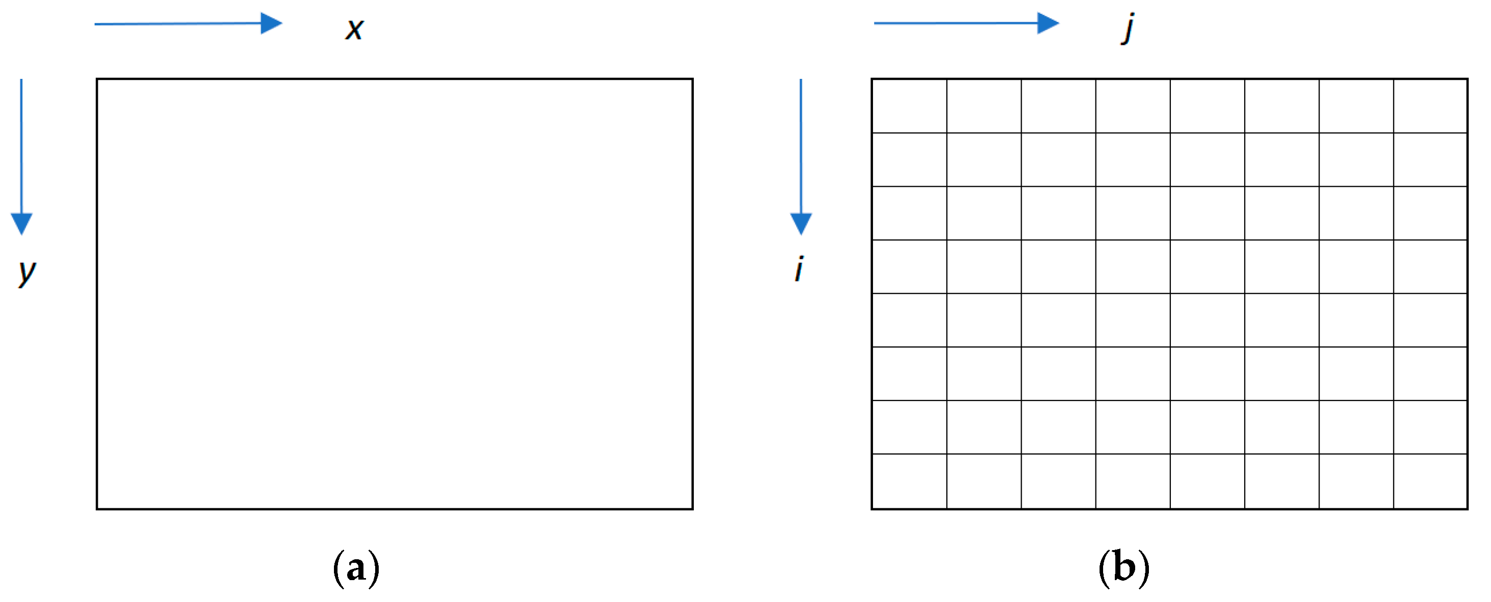
It is necessary to explain how a picture is perceived in a digital environment for a better understanding of the subject. An image can be defined in the simplest way as a 2-D function. Let’s call this function
. The
and
values found as parameters in the function represent plane coordinates. This value is also referred to as amplitude,
gray level, density, or brightness in any coordinate couple [
27]. An image needs to be digitized to be processed on a computer. As shown in
Figure 1,
and
parameters in
are integer values in a digitized image.
A digitizer is required to obtain an appropriate digital version of an image in the computer environment. In this context, the most commonly used digitizers are scanners and digital cameras.
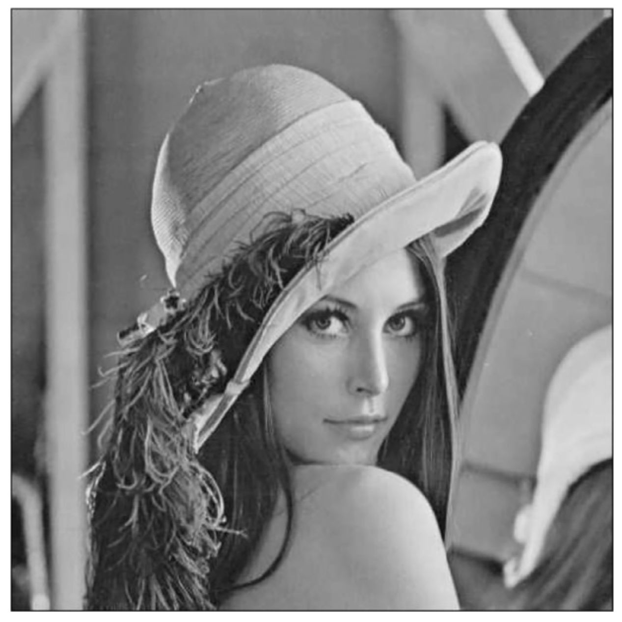
Images that use only light intensity are called grayscale images. The pixel on the image is a scalar proportional to the brightness. Grayscale images allow 256 color combinations, because the pixels use an 8-bit unsigned integer value that can be set between 0 and 255. An example of a grayscale image is shown in
Figure 2.
According to the Young–Helmholtz theory of color vision, color images are represented by the master colors red, green, and blue [
28]. The color space is obtained by linear combinations of these three main colors. Each color image scales the color and intensity of the light so that each color pixel represents a vector of color fragments. There are color spaces commonly used in the printing industry such as CMYK (cyan, magenta, yellow, and black), RGB (red, green and blue), and HSV (hue, saturation, and value) [
9]. Color images consist of three matrices, each with 8-bit values. These matrices represent the coordinates of each pixel in other color fields. That is, each pixel has a 24-bit sensitivity value, which is defined as 24-bit color.
The encoding phase is one of the most important steps in compression algorithms. The most important algorithms used in this field are the Huffman encoding algorithm and the arithmetic coding algorithm. Although the arithmetic coding algorithm has been developed to improve the efficiency of the Huffman encoding algorithm, it has deficiencies in mathematical processing and complexity. Therefore, there is a need for a new encoding algorithm that is more efficient and offers more successful compression results. The aim of this study is to develop an effective encoding algorithm suitable for all compression algorithms. The Huffman encoding algorithm and arithmetic coding algorithm are frequently used coding algorithms in the kernel of compression algorithms. Here, a new encoding algorithm has been developed that uses the advantages of the Huffman encoding algorithm and will eliminate the gaps of the arithmetic coding algorithm. The proposed encoding algorithm uses a modified tree structure from the Huffman encoding algorithm. After modification, a group of process is applied to the image to achieve a higher compression ratio and a lower number of bits per pixel. Since the deficiencies in the coding algorithms are addressed in this new algorithm, it will bridge the gap in the literature. This encoding algorithm will contribute to the literature and will likely be preferred in the compression algorithms to be developed.
The remainder of the paper is organized as follows:
Section 2 describes the technical background that is used in this work. In
Section 3, the proposed encoding algorithm is described with the necessary equations, representations, and step-by-step workflow. The experiment simulation and analysis of the proposed encoding algorithm is detailed in
Section 4.
Section 5 describes the results and discussion part of this work. In
Section 6, the paper is concluded with a general summary of the study.
2. Technical Background
2.1. Huffman Encoding Algorithm
The Huffman encoding algorithm is one of the most commonly used data compression methods in the field of computer science. The algorithm developed by David Huffman [
29] is used to reduce coding redundancy without loss of data quality. The use of data frequency is the basic idea in the Huffman encoding algorithm. The approach in the algorithm assigns symbols from the alphabet with variable codewords according to their frequency. The symbol with a higher usage frequency is symbolized by shorter codes in order to obtain a higher compression result. The steps for the Huffman encoding algorithm can be defined as follows:
Step 1: The frequencies of the symbols found in the data and the possibilities of the usage are listed. These possibilities are listed in a descending order from the highest to the lowest. A node is formed as a binary tree with the obtained probabilities.
Step 2: The lowest two probabilistic symbols contained in the cluster are retrieved. These two values are aggregated, and a new probability is generated. All the possibilities are regulated by a descending sequence.
Step 3: A parent node is created, marking the left branch as child node 1 and the right branch as child node 0, respectively.
Step 4: To create a new node, the two nodes with the smallest probabilities are changed, and the tree list is updated. If there is only one node in the list, then the process ends. Otherwise, Step 2 will be repeated.
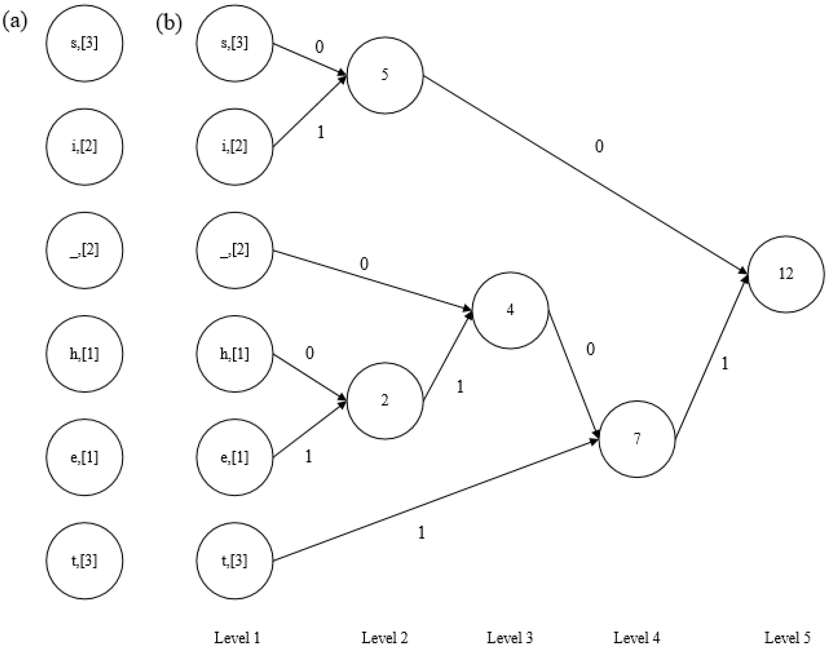
The Huffman algorithm is illustrated by an example below.
Let’s take the text ‘this_is_test’ and compress it with Huffman encoding. In the first step, the frequencies of each symbol (letter in the sample) in the text are counted. The frequency of the letters in the sample text is shown in
Table 1.
In the next step, nodes are generated according to the frequencies of the symbols. As shown in
Figure 3a, each node created at this stage stores a symbol and the frequency of that symbol, e.g., (i, [
2]) demonstrates that the ‘i’ symbol has a frequency of two in the text.
The previously created nodes are updated in the second step of the algorithm, as described below. As illustrated in
Figure 3b, the nodes of the letters with the lowest frequencies are selected. The nodes with the lowest frequencies that are randomly selected from Level 1 are combined to generate a new node at a higher level (Level 2). The value of the newly created node is equal to the total value of the frequencies of the merged nodes. Merging the nodes with the lowest frequencies continues until the root node is obtained.
In the third step, the links connecting the nodes are labeled with the values “0” and “1”. Here, connections on the left side are usually marked with a value of “0”, and connections on the right side are marked with “1”. In this way, a symbol is represented by an access path ending at the lowest level node starting from the root node. The access path from root to leaf node is called the Huffman code. The Huffman codes, based on the codeword, used in the example are shown in
Table 2. All symbols are replaced by Huffman codes.
The compressed bit sequence, obtained as a result of replacing the symbols in the example used with the Huffman codes, is tabulated in
Table 3. At the stage of rebuilding a compressed file, the Huffman tree is regenerated from the frequencies of the symbols and converted into the original characters. The bit stream is used to traverse the Huffman tree. Each iteration is monitored from the root node until it reaches the node of that symbol. This procedure starts all over again for the next node.
In cases where a small number of symbols are used and there are small differences in the probability of characters, the efficiency of Huffman encoding is reduced. Thus, arithmetic coding is needed to handle this problem.
2.2. Arithmetic Coding Algorithm
Arithmetic coding is one of the most used data compression methods in the literature that decreases coding redundancy, like Huffman coding [
30]. It creates a code string that symbolizes fractional values between 0 and 1. The fundamental idea used in arithmetic coding is to divide the values from 0 to 1 according to the probability of the symbols in the message. When the symbol count is small and there are less differences in the probability of the characters, Huffman encoding loses its effectiveness, while arithmetic coding is more successful. In arithmetic coding, each series must be labeled with a unique identifier to separate a particular set of symbols from other symbols. This tag is usually defined as a number between 0 and 1 [
31,
32,
33,
34,
35].
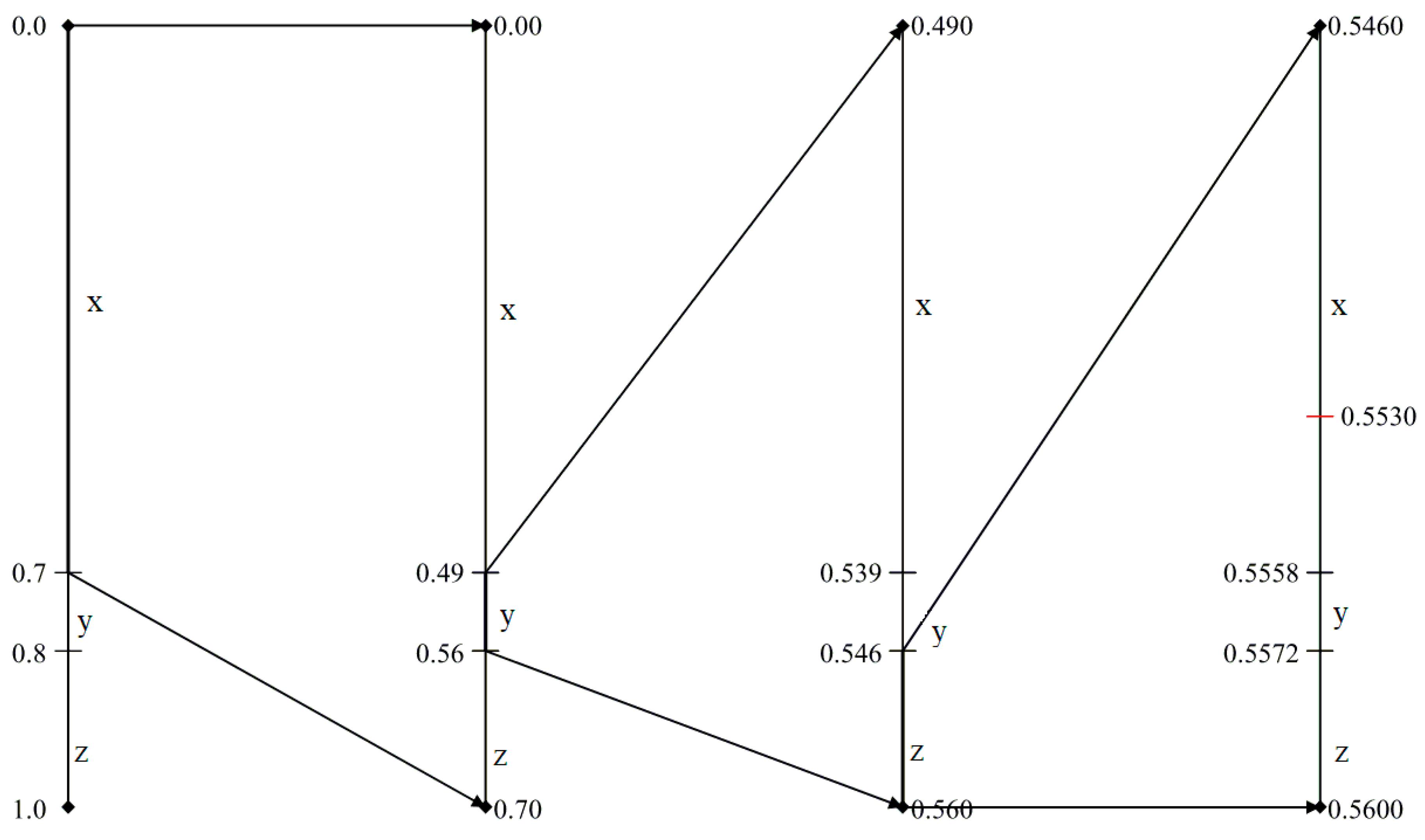
For example,
Table 4 presents the text ‘xxyxxzxzxx’ compressed using arithmetic coding, as seen in [
36]. The text consists of three letters,
, the alphabet. The probability distributions of this text are P(x) = 0.7, P(y) = 0.1, and P(z) = 0.2, as shown in
Table 4.
To find the tag for the series of letters x, y, and z, it is first necessary to divide it into 3 different parts based on the probability distribution between 0 and 1. The letter x is allocated from 0 to 0.7, y from 0.7 to 0.8, and z from 0.8 to 1. Since the first character of the series is x, the range allocated to x is expanded from 0 to 0.7 when the second character is passed. The new interval is divided into three different parts based on repeat probability distributions. The letter x is now allocated from 0 to 0.49, y from 0.49 to 0.56, and z from 0.56 to 0.7. Since the second character of the series is y, the process is continued by selecting 0.49 to 0.56. The third character of the series, z, will allocate between 0.546 and 0.56, and any numerical value within this range can be selected as the label of the series. The diagram of the determination of alphabetic arithmetic coding labels is shown in
Figure 4. In the figure, the steps of this process are shown from left to right. As shown in the figure, the midpoint of the last range in this example, 0.553, was selected as the label.
Arithmetic coding addresses some deficiencies in the Huffman encoding algorithm, however, there are also significant disadvantages in arithmetic coding. The main disadvantages of arithmetic coding are: (1) it is difficult to implement, (2) it does not generate prefix code, and (3) the algorithm execution is very slow. Such difficulties can be overcome, but the lack of a prefix code is a notable disadvantage, possibly leading to fault resistance.
3. Materials and Methods
Some criteria have been used to better understand the developed algorithm and to evaluate its success. These criteria are presented in this section of the manuscript.
3.1. Image Compression
Image compression is a very popular research topic in the field of computer science. An image can be compressed according to its correlation between the neighboring pixels in an image. This correlation between adjacent pixels on the image is called redundancy. There is a significant redundancy between images taken from multiple sensors, such as medical or satellite images. In other words, compression is performed by using the redundancies on the image. In addition, a more efficient compression ratio is obtained if the existing redundancies are removed prior to compression.
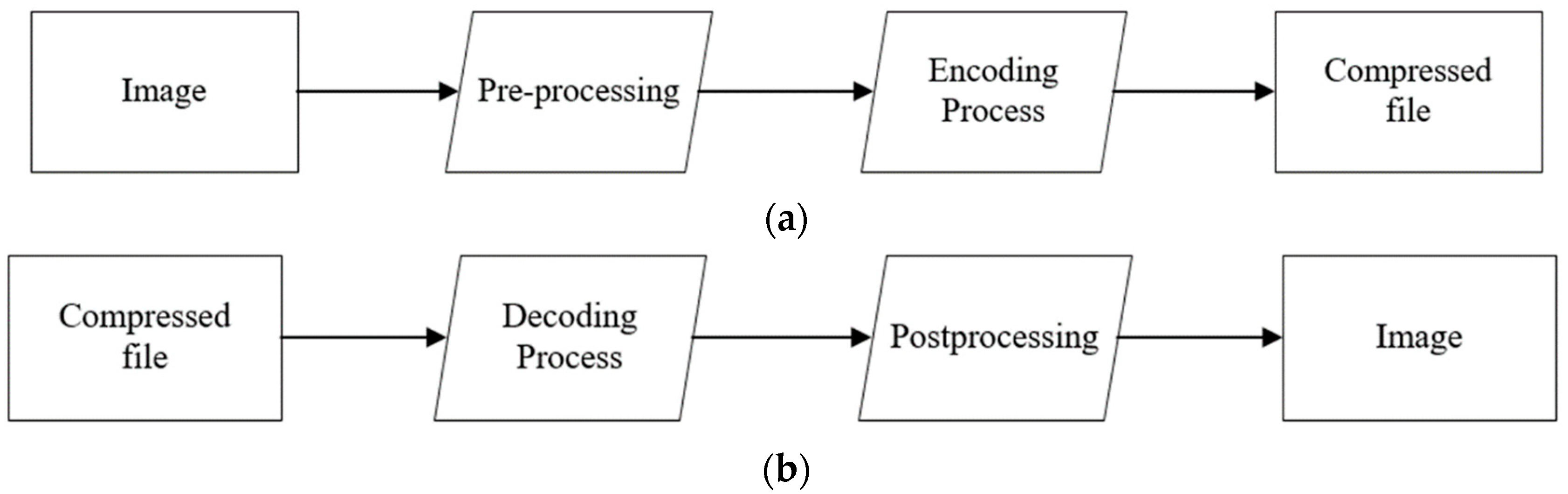
Compressor and decompressor operations generate an image compression system. The compressor process consists of two stages: preprocessing and encoding. Unlike the compressor process, the decompressor operation consists of the postprocessing phase after the decoding process. The flowchart of the compression process is shown in
Figure 5. As shown in the compression process, the pre-processing step, which differs based on the application, is applied before the coding step. In the reverse process, the postprocessing step can be applied to eliminate some of the residues from the compression process after the compressed code has been decoded.
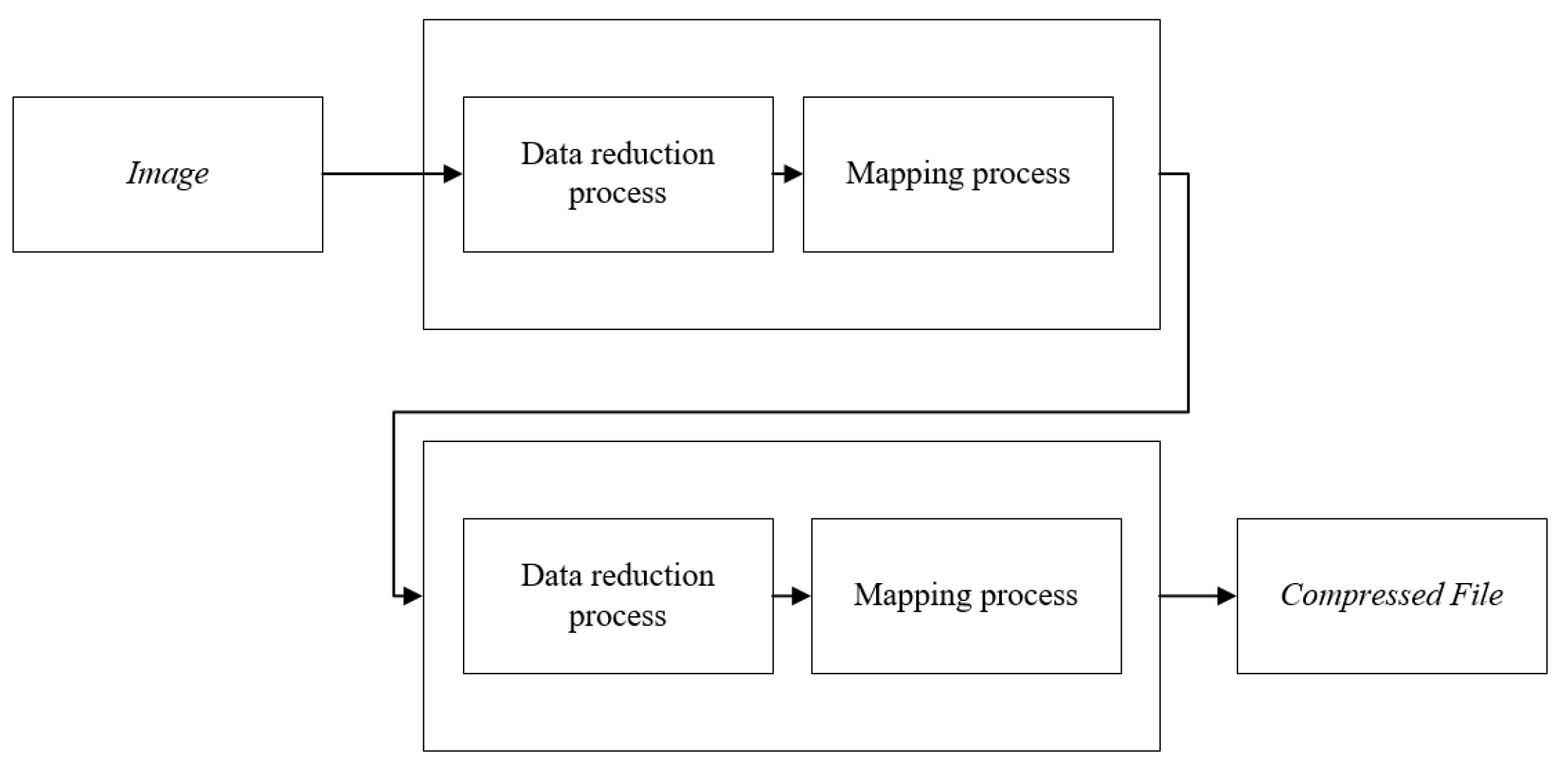
The compression process can be subdivided into the stages shown in
Figure 6. Data reduction is the first step of pre-processing. At this stage, image enhancement processes such as noise removal can be applied, or image quantities can be reduced. The second step of this phase is the mapping process. With this process, the data is mapped to the mathematical field for easier compression. Quantization steps are then applied as part of the encoding process. Data are stored in discrete form by the quantization stage. As the last process of the encoding step, the obtained data is coded. A compression algorithm may include one, or all, of these stages.
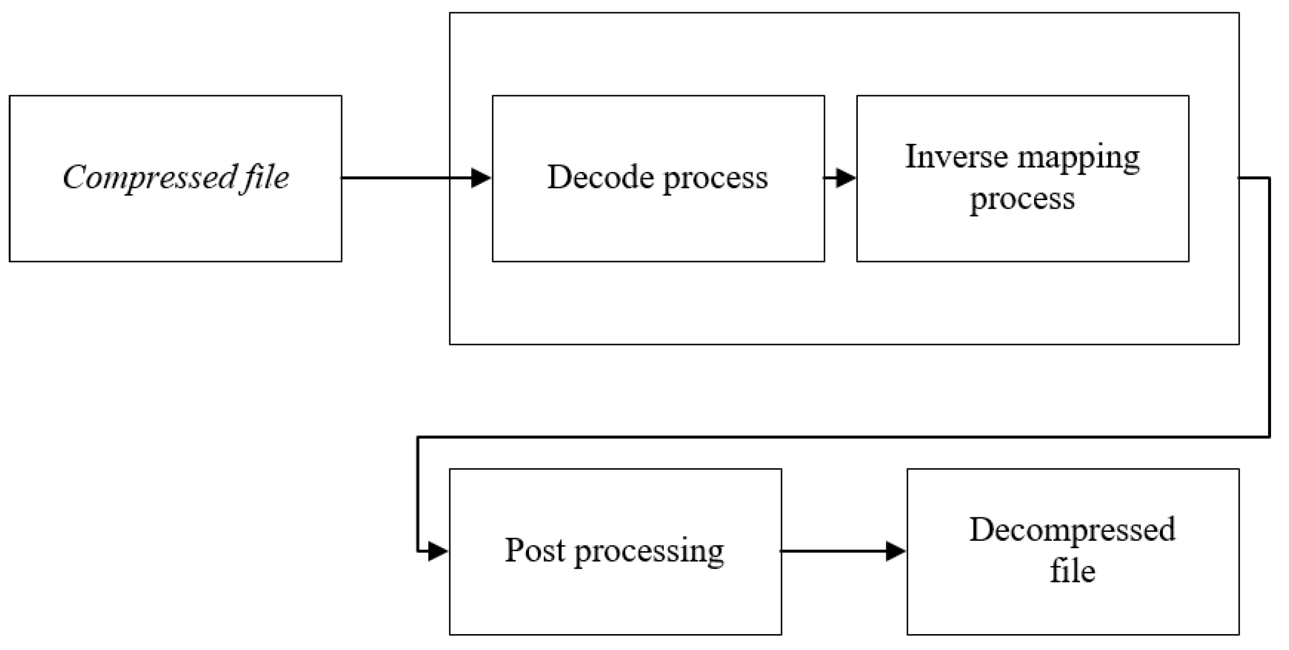
The decompression process can be subdivided into the stages shown in
Figure 7. The decoding process consists of two steps. In the first stage of this process, it matches the codes in the compressed file with the original values and reverses the encoding. The values obtained after this step are processed, and the original mapping process is reversed. At the end of these processes, the image can be improved with a post-processing step.
A compression algorithm is generally developed according to the application requirements. In the pre-processing step of the compression algorithm, operations such as noise removal, quantization, or development are applied according to the requirement. The main purpose of this process is to eliminate any irrelevant or unnecessary information that will affect the operation of the application, and to make the image ready for the encoding step.
The coding stage has an essential role in the image compression algorithm. A one-to-one mapping process is provided at this stage. This step is a reversible process, and each input must match a unique output. The code to represent each input may be of the same length or may be of different lengths. Usually, an unequal length code approach is the most appropriate method used in data compression [
37].
3.2. Image Compression Measurement
The file obtained as a result of compression is called a compressed file. This file is used to restore the image to the original. The compression percentage is the data that shows how the original file is compressed. The process used to obtain the compression percentage is shown in Equation (1). The compression percentage (CP) will be used in all comparisons during this study.
Another term used in this field is the number of bits per pixel (NoBPP). The method of calculating this value for an image with N × N dimensions is shown in Equation (2).
The aim of this study was to develop an effective encoding algorithm suitable for all compression algorithms. The Huffman encoding algorithm and arithmetic coding algorithm are frequently used coding algorithms in the kernel of compression algorithms. Here, a new encoding algorithm was developed that used the advantages of the Huffman encoding algorithm, and eliminated the gaps in the arithmetic coding algorithm. The proposed encoding algorithm used a modified tree structure from the Huffman encoding algorithm. After this modification, a group of processes was applied to the image, then, a higher compression ratio and a lower number of bits per pixel were achieved. Since this new coding algorithm addressed deficiencies in the other coding algorithms, it bridged the gap in the literature.
3.3. Proposed Algorithm
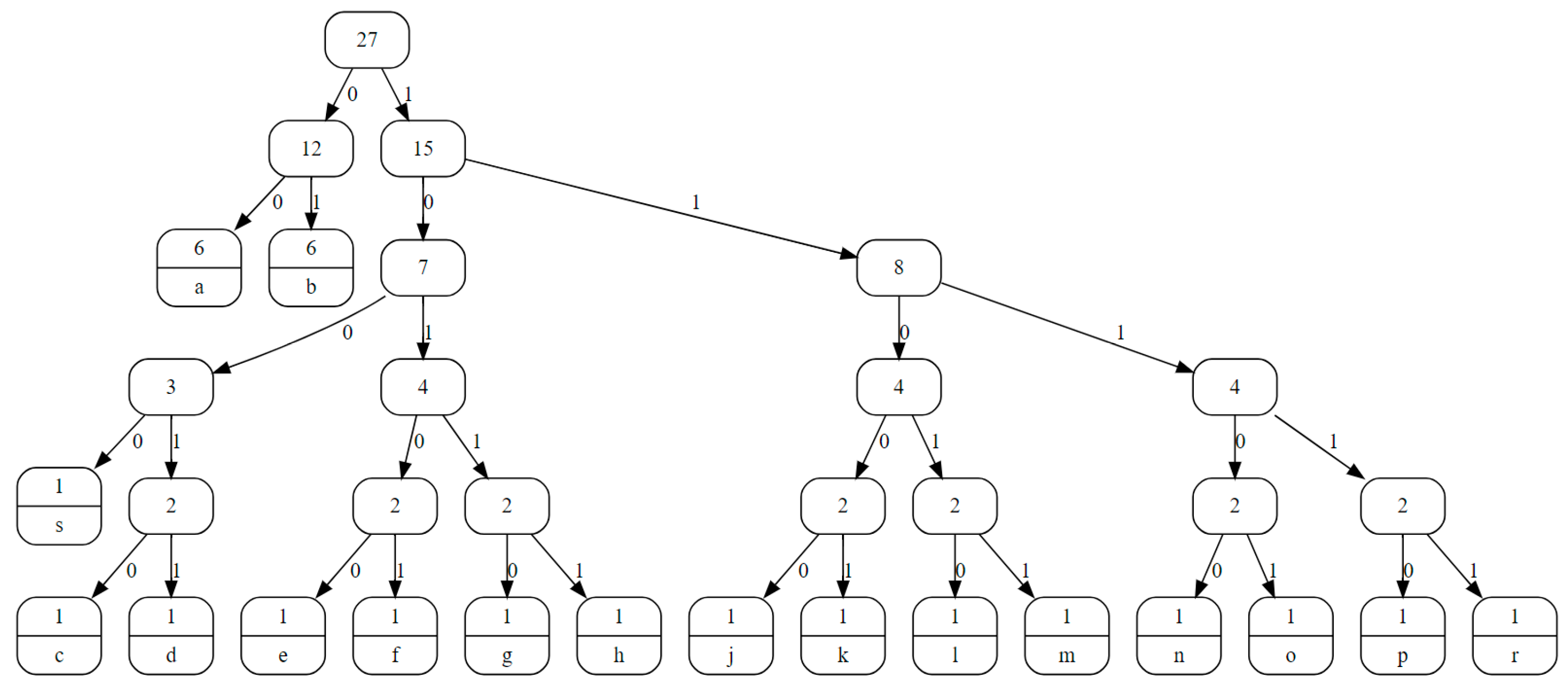
To better explain the proposed algorithm, an example follows. The text ‘aaaabbbbcdefghjklmnoprsaabb’ is used. For a better understanding of the developed algorithm, a sample special sequenced text is selected. However, in the experimental results of the study, the algorithm is tested with the data used in the literature. The number of times each character is used in text is defined as the frequency of these characters. In the text used in our example, ‘a’ is used 6 times, and ‘c’ is used 1 time. The frequency table for each character in the text is tabulated in
Table 5 below.
The Huffman tree of the text is formed, as shown in
Figure 8. To produce a bit codeword of each character, the Huffman tree is traversed from the root to the leaf node where the target character is located. For example, in order to reach the character ‘c’, the sequence of 10010 bits must be followed, respectively. In addition, each character symbolized by the Huffman encoding algorithm is presented in
Table 6.
If only the Huffman encoding algorithm is used to compress the text used in the example, a 98-bit sequence would be generated as follows:
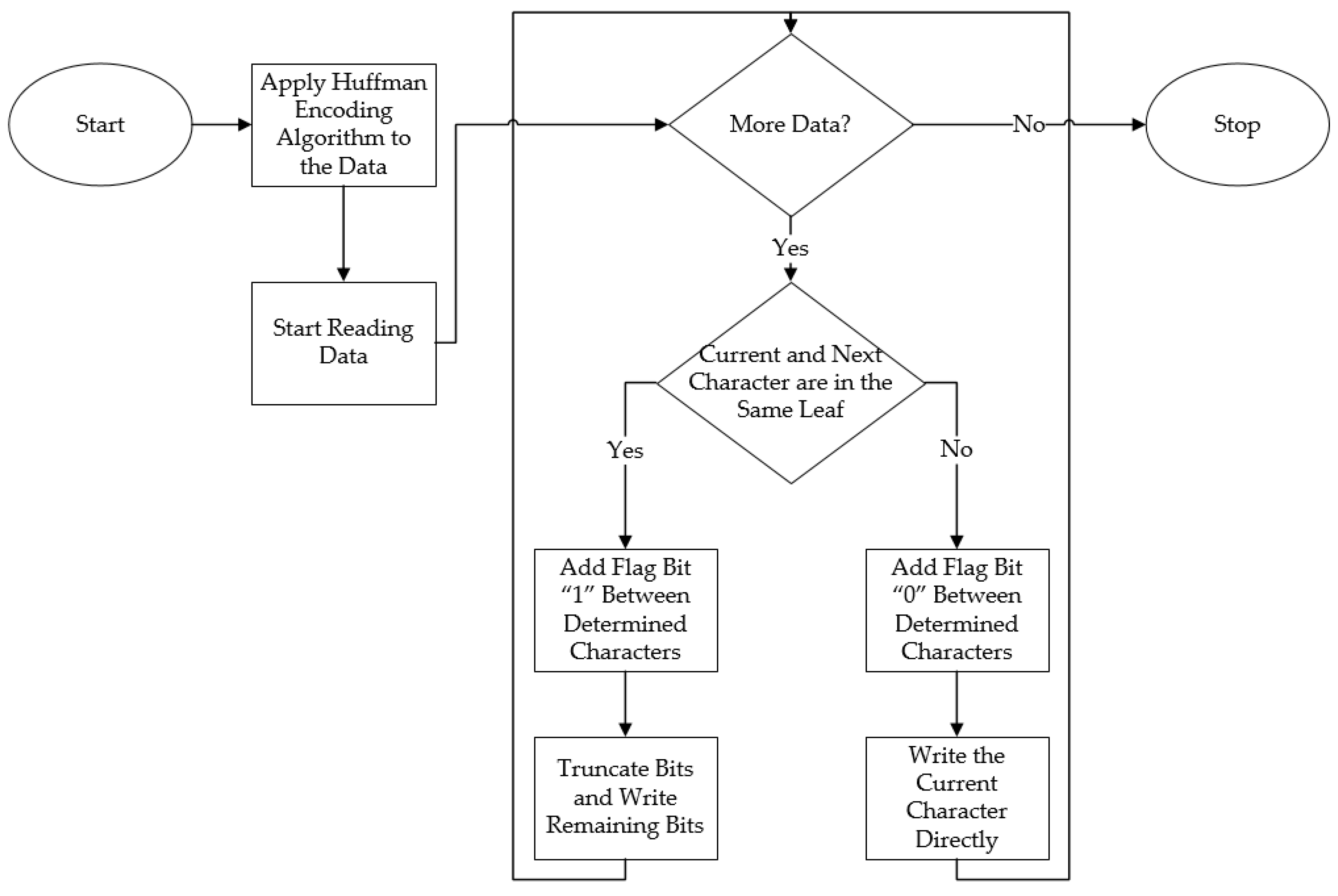
The main objective of the proposed algorithm, and all compression algorithms, is to reduce the number of bits needed to symbolize the characters. The flowchart of the proposed method is shown in
Figure 9.
The developed encoding algorithm is outlined in the following steps:
Step 1: The Huffman encoding algorithm is applied to the data.
Step 2: Characters represented by large bits are identified, and characters represented by small bits are ignored. In this example, ignored characters are ‘a’ and ‘b’. Because the Huffman coding algorithm ideally symbolizes these characters with 2 bits, further compression of these characters is not possible.
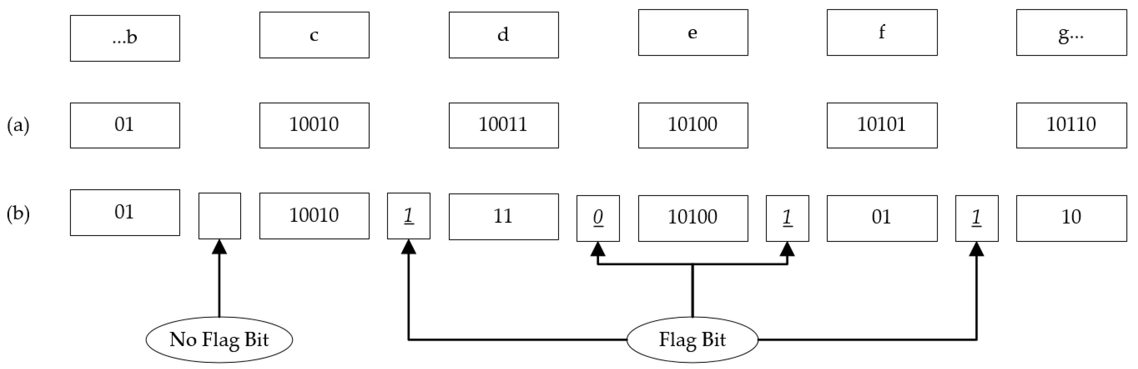
Step 3: Flag bits identified as 0 or 1 are added between characters represented by long bits. Flag bit “0” is added between determined characters if the current character and next character are not in the same leaf. Flag bit “1” is added between determined characters if the current character and next character are in the same leaf. That means there is no need to go through the entire Huffman tree to reach the next character. In
Figure 10, an example bit sequence from the text “…bcdefg…” is shown.
Figure 10a shows the Huffman encoding algorithm and
Figure 10b indicates the bit sequence of the specified section.
Step 4: When the flag bit represents the characters on the same node, there is no need to repeat the first three bits common in these characters. In this step of the algorithm, the first three bits of the characters on the same node are truncated and the bit sequence is rebuilt.
When the example text data is rearranged by the developed encoding algorithm, the resulting bit sequence is as follows:
As mentioned previously, special text was used to better understand the developed algorithm. This text was represented by 98 bits when compressed by the Huffman encoding algorithm. When the developed encoding algorithm was used to encode the text, it was represented by 83 bits. For this specific example, the developed coding algorithm achieved a better compression ratio of 15.30% compared to the Huffman encoding algorithm. In the next step of the study, detailed tests are performed on the data used in the literature to better evaluate the proposed encoding algorithm.
4. Simulation Experiments
The performance of the proposed encoding algorithm was tested on three different sets of pictures. In the first group, eight randomly selected images, frequently used in the literature from USC-SIPI [
38] miscellaneous databases, were chosen to prove the efficacy of the proposed coding algorithm. The sample images selected from the database included color and grayscale images in order to prove the performance of the encoding algorithm, and are shown
Figure 11.
These images were compared with the Huffman encoding and arithmetic coding algorithm results. Results are tabulated in
Table 7. Equation (1) was used to calculate the CP and Equation 2 was used to calculate the NoBPP of each algorithm per image.
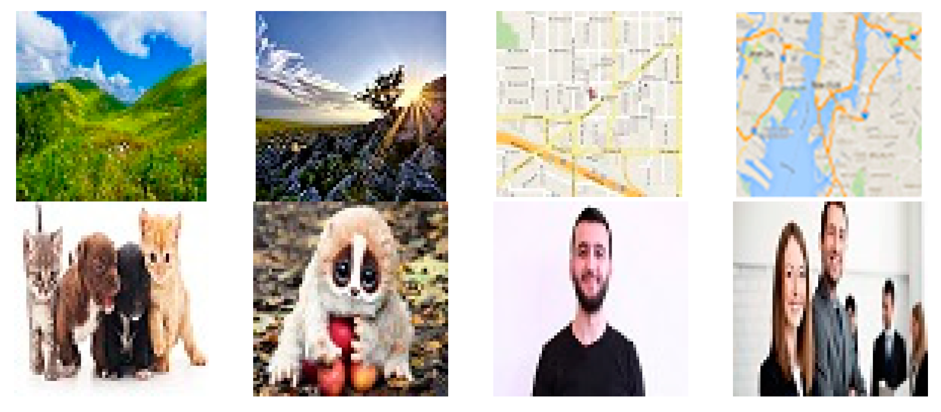
The second group of images used in this research included images of nature, maps, animals, and people, all chosen from the internet randomly and with different characteristics. The images used in the evaluation of the performance of the proposed coding algorithm are shown in
Figure 12.
The same algorithms were applied to this group as in the first group of images. The characteristics of the images and the results of the CP and NoBPP are listed in
Table 8.
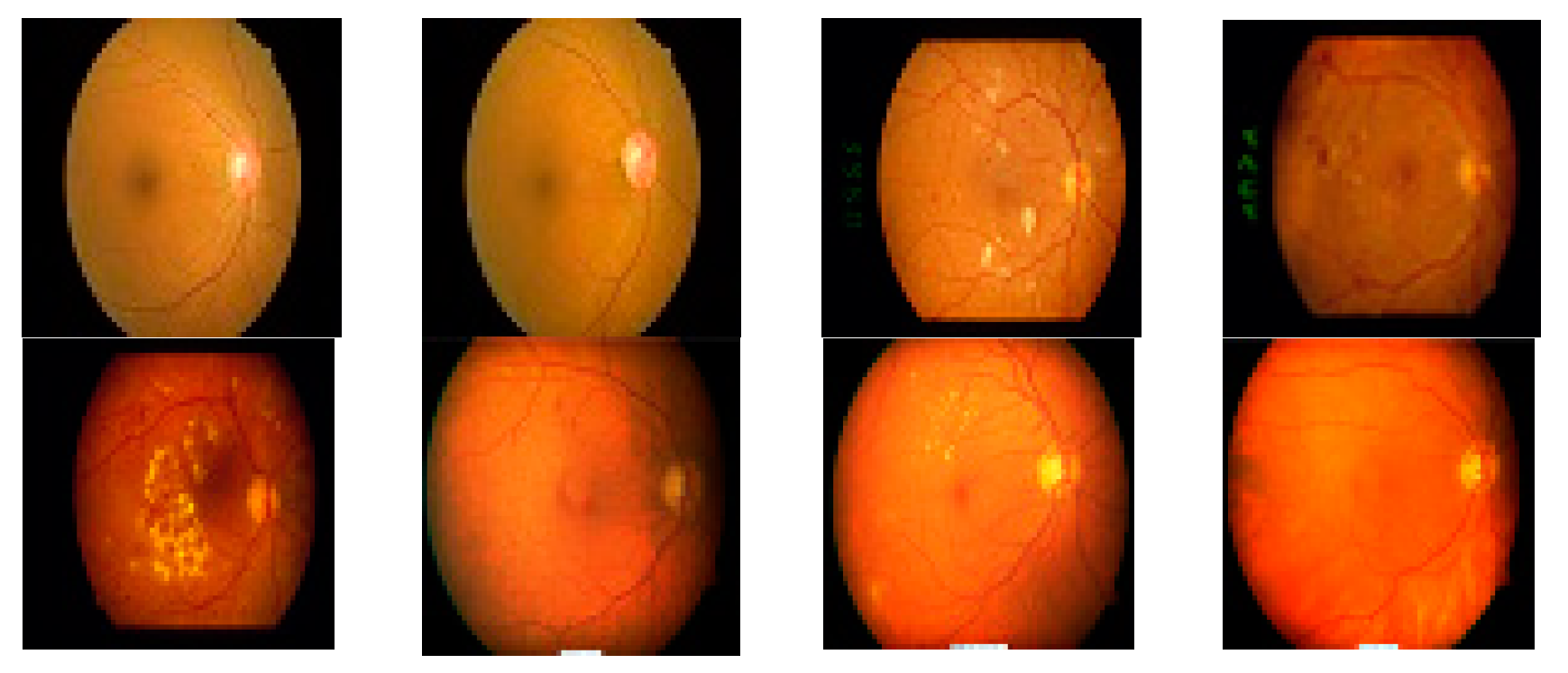
The third group of images used in the evaluation of the developed encoding algorithm included medical images. Medical image compression is frequently studied in the literature because these images have large file sizes and increasing image sizes. Retinal images are preferred as medical images in compression. The test images were taken from the Structured Analysis of the Retina (STARE) [
39] database, as shown in
Figure 13.
The algorithms were run on eight raw, randomly selected images from the Structured Analysis of the Retina database [
39], and the results are presented in
Table 9.
In the evaluation of the algorithm, images in three different groups were used. The developed encoding algorithm was compared with the Huffman encoding algorithm and arithmetic coding algorithm for evaluation. The results are presented in tables with CP and NoBPP values. The obtained results were analyzed in detail in the next step of the study.
5. Discussion of Results
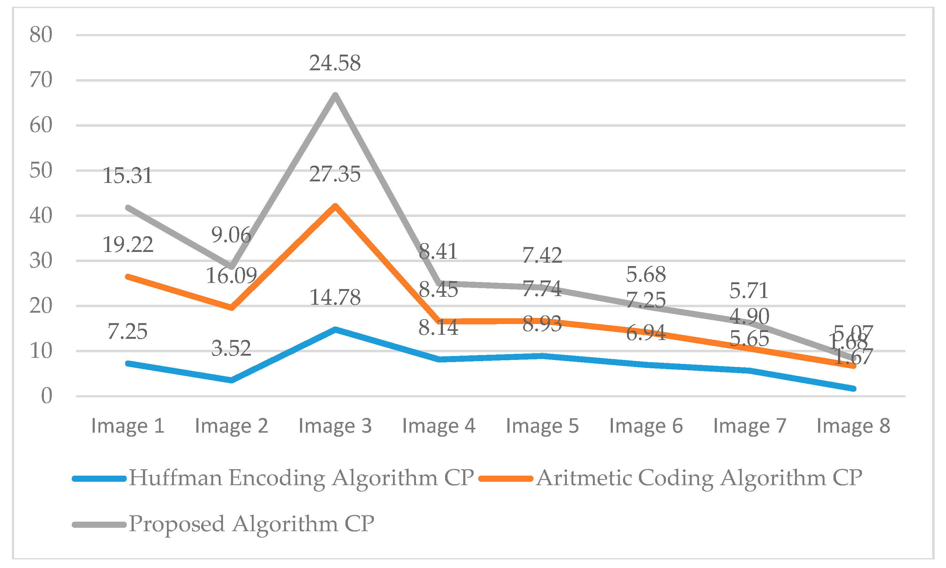
CP and NoBPP were terms both used in the scope of the study. First, CP values of each group were analyzed. Then, NoBPP values were evaluated. The CP values of the first group of images from Huffman encoding algorithm, arithmetic coding, and proposed algorithm are summarized in
Figure 14.
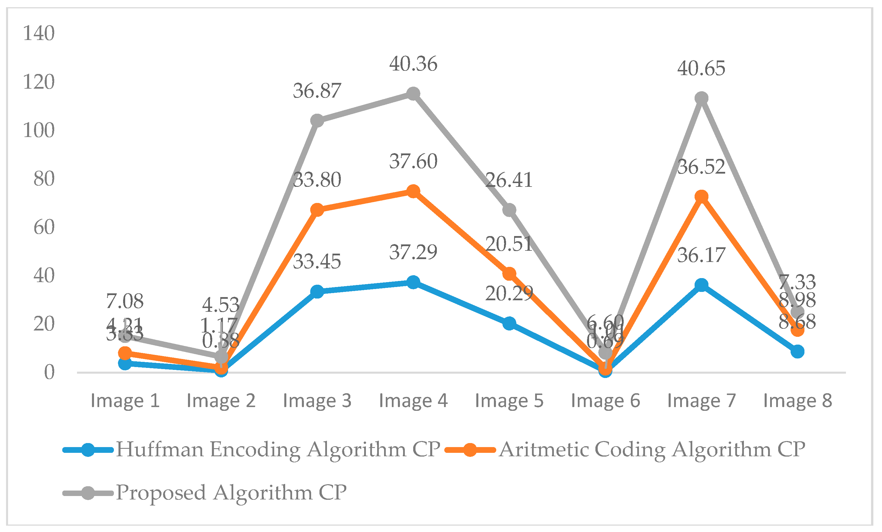
The CP values of the second group, with randomly selected images from the internet, are depicted in
Figure 15. It was observed that the proposed algorithm was better in the second group of images compared to the first group of images.
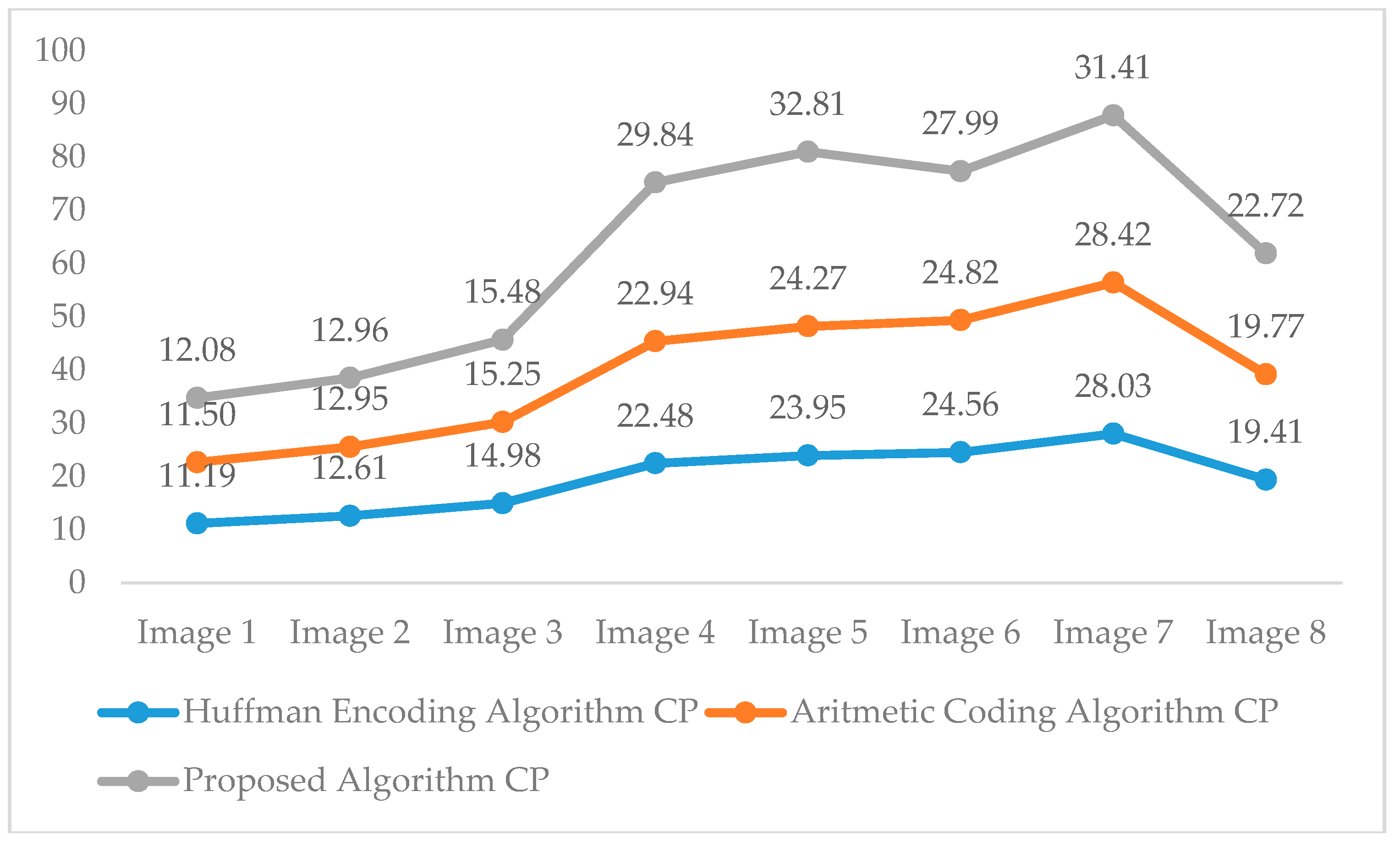
Medical image compression is a frequently studied area in the literature. Therefore, the proposed algorithm was also tested on medical images. The CP values of the third group of images is shown in
Figure 16.
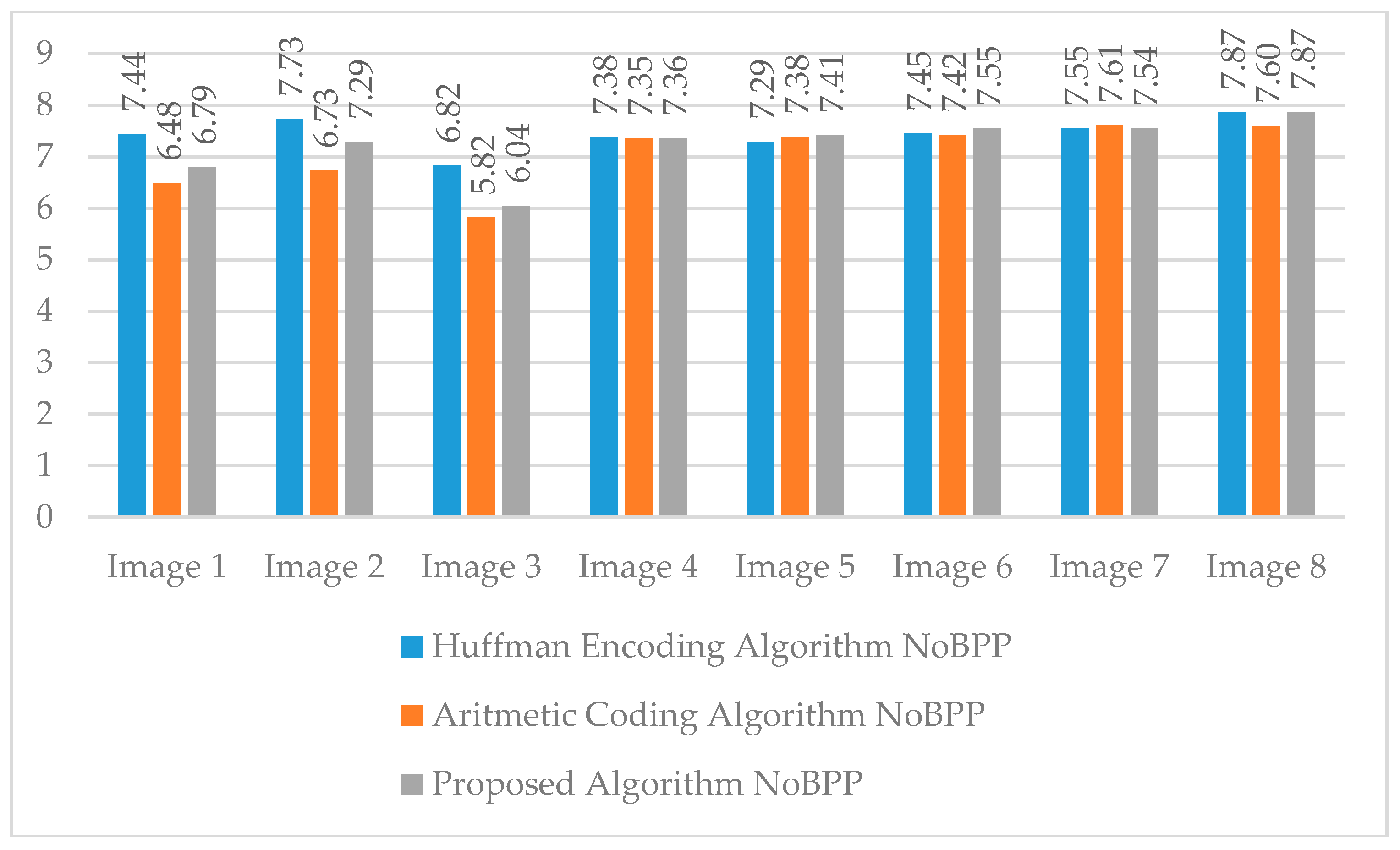
The second term used in the evaluation phase of the proposed encoding algorithm was NoBPP. The main purpose of compression algorithms is to reduce the bits per pixel. Therefore, the NoBPP value is used for more consistent and accurate results. The NoBPP value is presented for each group of images. NoBPP values obtained from the algorithms applied to the first group of images are shown in
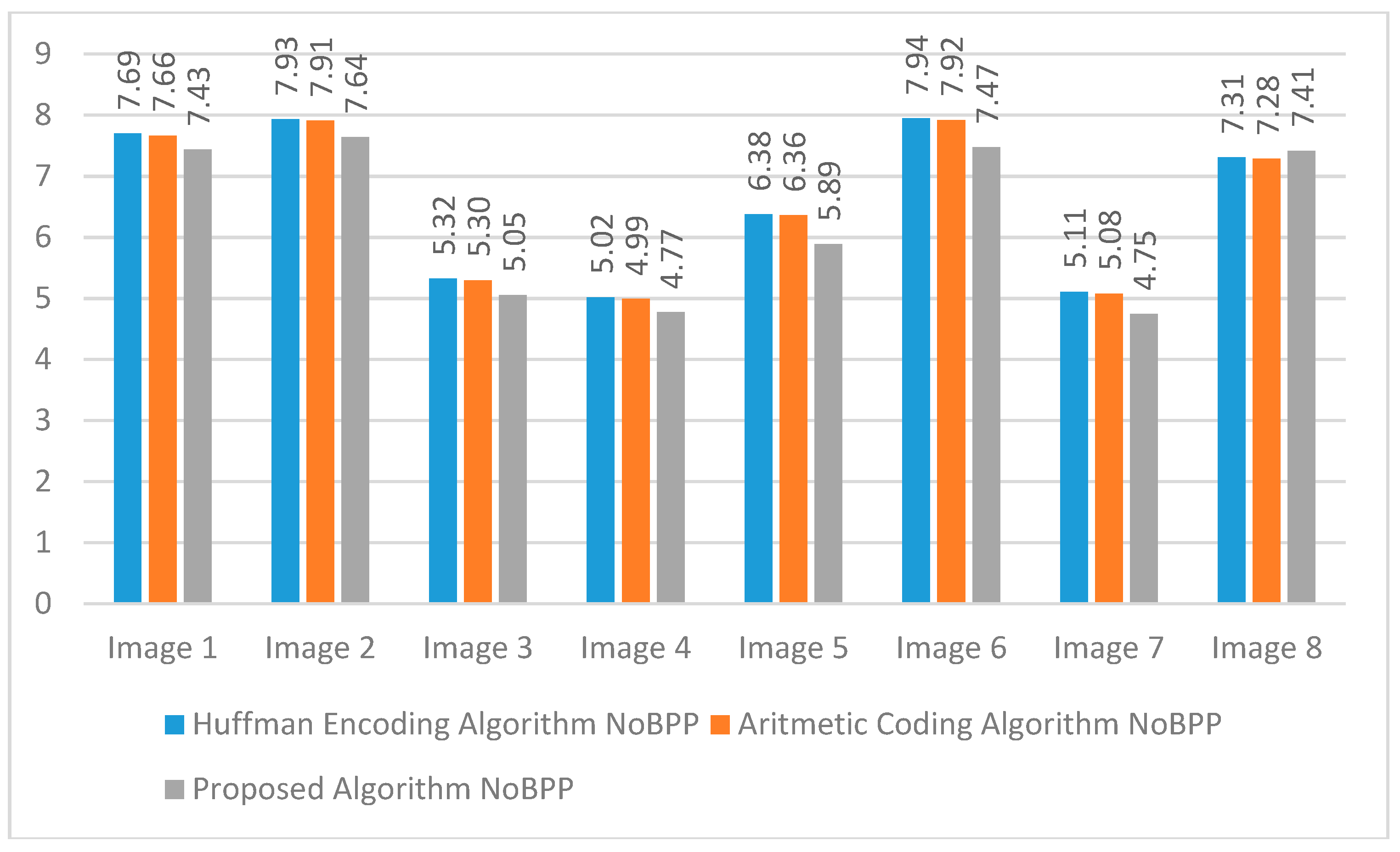
Figure 17. The NoBPP values of the images in the second group are presented in
Figure 18.
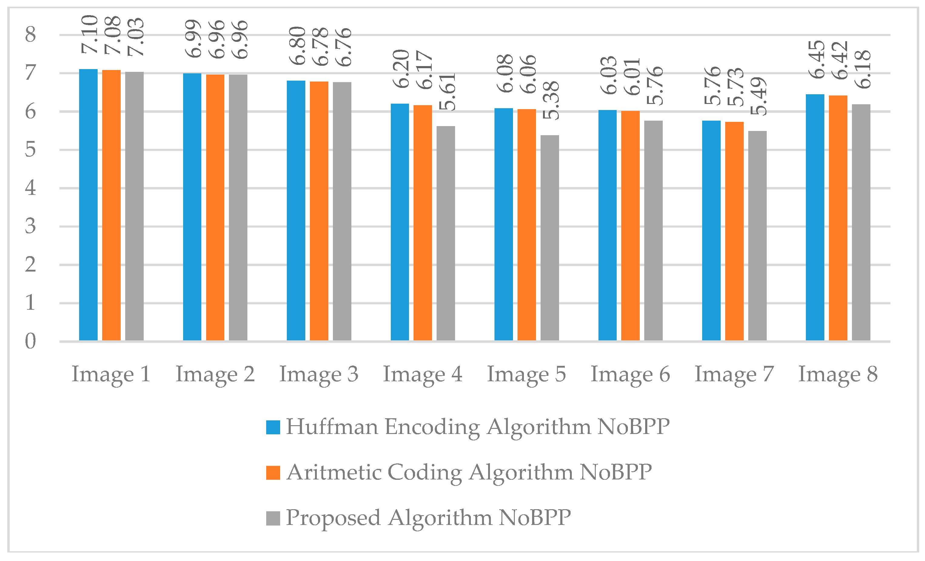
NoBPP values from the third group of images containing medical images are depicted in
Figure 19. As seen from the data, in the first group of images the proposed encoding algorithm showed better CP and NoBPP values than the Huffman encoding algorithm. However, it lagged slightly behind the arithmetic coding algorithm. The developed encoding algorithm provided better CP and NoBPP values in the second group of images compared to both the Huffman encoding and arithmetic coding algorithms. In the last group, where medical images were used, the developed coding algorithm showed better CP and NoBPP values. Considering these values, the developed encoding algorithm performed better than the algorithms in the core of many image compression algorithms. The resultant compression performance was better than arithmetic coding, which proves the success of the developed encoding algorithm. It offered fast runtimes and was easy to implement due to the use of only the Huffman encoding algorithm tree structure.
When analyzing the success of the image groups, it was seen that the developed encoding algorithm provided better results in the images under the following conditions:
When the Huffman tree had an unbalanced tree structure. Otherwise, results were similar to (or better than) the Huffman Encoding Algorithm.
In images where the same pixels were as consecutive as possible over the image, e.g., the map images in the second group, all medical images in the third group, and the images of the candies and the man in the first group.
When there was a lower number of characters in the image. Although the number of different characters in medical images is high, our algorithm gave more successful results. This is because consecutive pixels are represented by the same local path, which is the advantage of our algorithm.
The main purpose of developing a new encoding algorithm is to provide an alternative solution to the algorithms where long characters are represented by long symbols, such as Huffman encoding or arithmetic coding. The developed encoding algorithm uses all the advantages of the Huffman encoding algorithm. In addition, it offers solutions to address the gaps in the Huffman encoding and arithmetic coding algorithms. Thus, the proposed algorithm bridges the gap in the literature.
6. Conclusions
Encoding algorithms, which are one of the most important steps in each compression algorithm, are studied extensively in the literature. The Huffman and arithmetic coding algorithms are used intensively in this field. The arithmetic coding algorithm has been developed as a more efficient alternative to the Huffman encoding algorithm. Despite its efficiency, the developed arithmetic coding algorithm is relatively slow, complex, and hard to implement. Therefore, a new coding algorithm was needed that is an efficient alternative to the arithmetic coding algorithm, and as fast as (and less complex than) the Huffman encoding algorithm.
In this paper, we present an alternative encoding algorithm for general compression purposes. The encoding algorithm that we proposed is based on the local path of the Huffman encoding algorithm. The proposed algorithm uses all the advantages offered by the Huffman encoding algorithm, but it also provides solutions to characters that require a long symbol. It also provides similar, or better, results with the arithmetic coding algorithm, which addresses the gaps in the Huffman algorithm. The proposed encoding algorithm also addresses deficiencies in the arithmetic coding algorithm such as implementation difficulties, slow execution times, and unnecessary production of prefix codes.
The success of the developed encoding algorithm has been tested on three different groups of images. Some images have similar results with the arithmetic coding algorithm and better compression performances than the Huffman encoding algorithm.
One of the most important criteria used in evaluating the success of the algorithm is the NoBPP value. From the experiments, we draw the following conclusions:
In Group 1 Images:
In Group 2 Images
In Group 3 Images
The obtained results show that the developed algorithm has better compression results in a variety of image types. We believe that the proposed algorithm bridges the gaps in the literature because the Huffman tree of the image can have an unbalanced tree structure, the same pixels are as consecutive as possible over the image, and the number of different characters needed was lower in the image.
Currently we are developing another encoding algorithm model that will improve this encoding algorithm. In the future, we are planning to: (1) develop a dynamic solution in accordance with the 3-bit sequence limit used in this solution, (2) implement a dictionary-based new effective encoding algorithm, and (3) at the end of these objectives, reveal an international architecture of an alternative lossless compression algorithm.


