Fully Symmetric Convolutional Network for Effective Image Denoising

Abstract

Neural-network-based image denoising is one of the promising approaches to deal with problems in image processing. In this work, a deep fully symmetric convolutional–deconvolutional neural network (FSCN) is proposed for image denoising. The proposed model comprises a novel architecture with a chain of successive symmetric convolutional–deconvolutional layers. This framework learns convolutional–deconvolutional mappings from corrupted images to the clean ones in an end-to-end fashion without using image priors. The convolutional layers act as feature extractor to encode primary components of the image contents while eliminating corruptions, and the deconvolutional layers then decode the image abstractions to recover the image content details. An adaptive moment optimizer is used to minimize the reconstruction loss as it is appropriate for large data and noisy images. Extensive experiments were conducted for image denoising to evaluate the FSCN model against the existing state-of-the-art denoising algorithms. The results show that the proposed model achieves superior denoising, both qualitatively and quantitatively. This work also presents the efficient implementation of the FSCN model by using GPU computing which makes it easy and attractive for practical denoising applications.

1. Introduction

Image denoising is an active topic in low-level vision since it is an indispensable step in many practical applications. The goal of image denoising is to recover a clean image from a noisy observation resulting in minimal damage to the image. In the past few decades, extensive studies have been carried out to develop various image denoising methods. Traditional image restoration methods rely on predefined image priors for image processing. Various models have been exploited for modeling image priors such as Nonlocal Self-Similarity (NSS) models [1,2,3,4], sparse models [5,6,7], gradient models [8,9,10], and Markov Random Field (MRF) models [11].

Despite their high denoising quality, most of these methods suffer from significant drawbacks where a complex optimization in the testing stage is required, thus making the denoising process time-consuming. These methods can hardly achieve high performance without sacrificing computational efficiency.

The above drawbacks are overcome by discriminative learning-based methods. Unlike in the traditional image restoration methods, the parameters of Deep Neural Networks (DNNs) are directly learned from training data (from the pairs of clean and corrupted images) rather than predefined image priors. Stacked Denoising Autoencoder (SDA) is one of the early deep learning models which has been used for image denoising [12]. However, it fails to learn anything useful if it is given too much large data. Sparsely connected Multilayer Perceptron (MLP) method has the advantage of being computationally easier to train and evaluate. However, the number of parameters in MLPs is often too large [13].

In deep learning, Convolutional Neural Networks (CNNs) are found to give the most accurate results in solving real-world problems. CNNs are widely used in various image-processing problems [14,15,16] and have achieved significant success in the field of image restoration compared to MLPs and autoencoders. CNNs with deep architecture are effective in increasing the capacity and flexibility for exploring image characteristics. For training CNNs, considerable advances have been achieved on regularization and learning including Rectified Linear units (ReLu) [17] and batch normalization [18]. By observing the recent superior performance of CNNs on image-processing tasks, we propose a deep fully symmetric convolutional–deconvolutional neural network for image denoising, which is referred to as FSCN hereafter. The proposed model comprises a novel architecture with a chain of successive symmetric convolutional–deconvolutional layers. The framework learns convolutional–deconvolutional mappings from corrupted images to the clean ones in an end-to-end fashion without using image priors. The convolutional layers act as feature extractor to encode primary components of the image contents while eliminating corruptions, and the deconvolutional layers then decode the image abstraction to recover the image content details. Our model achieves very appealing computational efficiency compared to other methods.

The content of the paper is organized as follows. Section 2 provides a brief survey of related work, Section 3 presents the architecture of the proposed FSCN model, Section 4 presents an extensive discussion of experimental results to evaluate the model, and the summary and prospects of the study are provided in Section 5.

2. Related Works

Extensive studies have been conducted to develop various image restoration methods. Traditional BM3D [2] algorithm and dictionary-learning-based methods have shown promising performance on image denoising despite relying on predefined image priors [5]. However, image prior knowledge formulated as regularization techniques [8] is effective in removing noise artifacts but tends to oversmooth images. The popular and dominant wavelet-based method introduces ringing artifacts in the denoised image. Application of spatiotemporal filters reduces noise but strong denoising causes blurring [19]. Bilateral filter smooths noisy images but leads to oversmoothing of images while preserving the edges [20]. However, direct implementation of a bilateral filter takes longer for one-megapixel images and does not achieve real-time performance on high-definition content. It also tends to oversmoothing and edge-sharpening. Joint distribution wavelet method was proposed [21] to remove noise from digital images based on a statistical model of the coefficients of an overcomplete multiscale-oriented basis. Nonetheless, this method introduced ringing artifacts and additional edges or structures in the denoised image. Talebi et al. [22] prefiltered the noisy image by using the bilateral filter and eigenvectors were approximated by using Nystrom and Sinkhorn approximation to decompose the prefiltered noisy image. However, the process could be very slow and complicated if the eigenvalues are estimated for a full image.

Currently, dynamic and promising neural-network-based methods have been explored in image denoising. Neural-network-based methods typically learn parameters directly from training data rather than relying on predefined image priors. Recently, there have been several attempts to handle the denoising problem by DNN. The early DNN-based SDA pretraining minimizes the reconstruction error with respect to input layers one at a time. The network goes through a fine-tuning stage when all layers are pretrained. Nevertheless, the focus turned out to capture the interesting structure for subsequent learning tasks which is different from that of developing a competitive denoising algorithm [12]. Agostinelli et al. [23] used Adaptive Multicolumn Stacked Sparse Denoising Autoencoder (AMC-SSDA) for image denoising. Each denoising autoencoder layer was trained by generating new noise using optimized weights which are determined by features of each given input image. It is effective for images corrupted by multiple types of noises but requires a separate training network to predict the optimal weights. MLPs are capable of dealing with various types of noise. Burger et al. [13] presented a patch-based algorithm learned on a large dataset with a plain MLP which could match with state-of-the-art traditional image denoising methods such as BM3D. However, the drawback of MLP is that every hidden unit is connected to every input pixel and does not assume any spatial relationships between pixels.

On the other hand, CNN has achieved more significant success in the field of image restoration compared to autoencoders and MLPs. CNN is used to denoise natural images wherein the network was trained by minimizing the loss between a clean image and its corrupted version produced by adding noise. CNN worked well on blind and nonblind image denoising showing superior performance compared to wavelet and Markov Random Field (MRF). Their framework is the same as that of a recently developed Fully Convolutional Neural Network (FCN) for semantic segmentation [24] and super-resolution [25]. Their network could accept an image as the input and produce an entire image as an output through four hidden layers of convolutional filters. Wang et al. [26] proposed a deep convolutional architecture for natural image denoising to overcome the limitation of fixed image size in deep learning methods. Their architecture is a modified CNN structure with rectified linear units and local response normalization, and the sampling rate of all pooling layers was set to one. It is noted that many denoising methods are patch-based algorithms where images are split into patches and denoised patch by patch [13]. Here, the patch size is an important parameter that affects the performance. For example, BM3D [2], Weighted Nuclear Norm Minimization (WNNM) [11], MLP [13], Cascade Shrinkage Fields (CSF) [27], and Denoising Convolutional Neural Network (DnCNN) [28] are some examples of patch-based algorithms. Patch-wise training is common but lacks the efficiency of fully convolutional training. Among many learning-based methods, the DnCNN [28] method has achieved competitive denoising performance. It showed residual learning and batch normalization are particularly useful for the success of denoising. Although CSF [27] shows promising results towards bridging the gap between computational efficiency and denoising quality, its performance is inherently restricted to the specified forms of prior. The parameters are learned by stage-wise greedy training plus joint fine-tuning among all stages.

Fully convolutional training is trained in an end-to-end fashion for pixel-wise prediction from supervised pretraining [24]. The fully connected layers are removed or replaced by FCNs so that the network becomes significantly smaller and easier to train compared to many other recent architectures [29]. Semantic segmentation [30] and image restoration [31] adopt fully convolutional inference. Tompson et al. [32] used FCN to learn an end-to-end part detector and spatial model for pose estimation. These methods have small models restricting capacity and receptive fields, and require postprocessing such as random field regularization or filtering while others require saturating tanh nonlinearities [30,31].

Most of the denoising methods proposed so far suffer from a few drawbacks despite the high denoising ability. The denoising process becomes time-consuming if a method involves complex optimization problems in the testing stage which would affect the computational efficiency. Although some methods find optimal parameters in a data-driven manner, they are limited to specific prior models [33]. Moreover, current CNN-based denoising networks are very deep, computationally very expensive to train, and time-consuming.

Therefore, we propose a method comprising a deep convolutional architecture with supervised pretraining and fine-tuned fully symmetrical convolution to learn efficiently from the whole image inputs. The key objective is to build a “fully convolutional” network which takes in arbitrary-size images and produces corresponding-size images with efficient inference and learning. The proposed work uses a unique FCN architecture for easier training with less time consumption while achieving better performance.

3. Deep Symmetric Convolutional–Deconvolutional Network

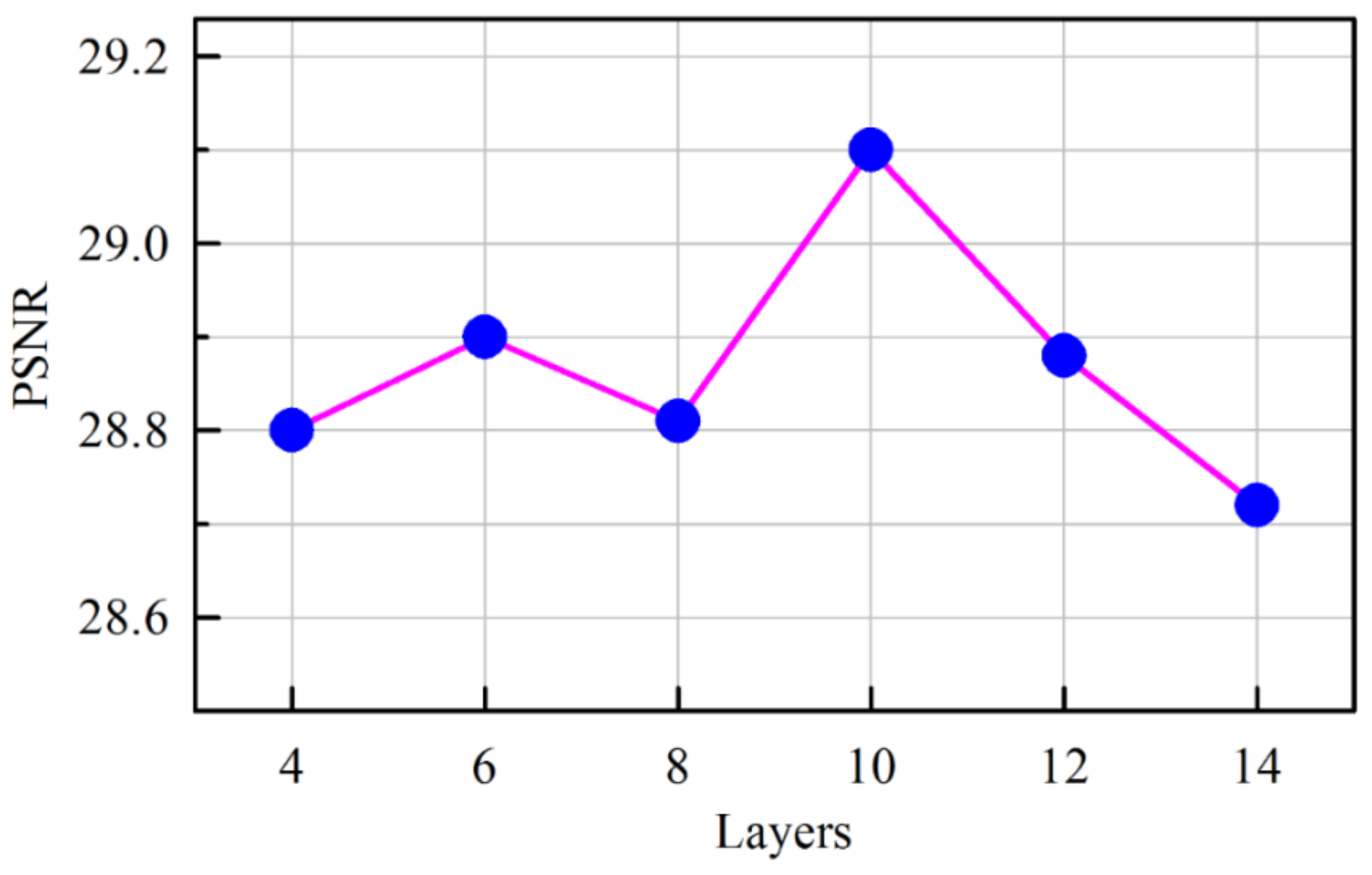
The proposed FSCN model for denoising is presented in this section. The FSCN model involves network architecture design and learning from training data. For network architecture design, fully symmetric convolutional–deconvolutional layers are used alternatively and the depth of the network is set based on the results. This architecture design aids in faster training and improved performance. The performance of the model is evaluated by comparing with other known networks. A visualization technique is employed to give insight into the function of intermediate feature layers.

3.1. FSCN Architecture

FSCN is a powerful visual model that yields hierarchies of features. The network trains end-to-end and pixel-to-pixel by itself. It learns convolutional–deconvolutional mappings from corrupted images to the clean ones without using image priors. Convolutional layers learn efficiently from image inputs and ground truths. It is fine-tuned from its learned representations, and the learned filters correspond to bases to reconstruct the shape of an input. It is used to capture the different level of shape details where the lower layers tend to capture overall shape while fine details are encoded in the higher layers. Deconvolution layers multiply each input pixel by a filter, and sums over the resulting output. Noisy activations are suppressed effectively while retaining the shape of the input by the deconvolution process. FSCN can separate the noisy observation from image structure through hidden layers by incorporating convolution and deconvolution layers with ReLu.

Figure 1 illustrates the skeleton of the proposed FSCN architecture for denoising. This architecture comprises a chain of successive symmetric convolutional–deconvolutional layers. The output of the architecture is an effective denoised image which has a noisy image input. Figure 2 demonstrates the details of the FSCN architecture. Each layer of data is a three-dimensional array of size h × w × c, where h and w are spatial dimensions and c is the channel or feature dimension. The first layer is the image with size h × w, and c = 1 for gray image and c = 3 for the color image. The FSCN architecture with depth N has two types of layers: (i) Convolution (Conv) with ReLu for odd layers and (ii) Deconvolution (Deconv) with ReLu for even layers. For Conv with ReLu layers located at 2l−1 position, (l = 1, 2, 3, 4, and 5) filters (f) of size m × n × c are used to generate feature maps (F) which are capable of achieving favorable performance in many computer vision tasks. Here, Conv layers act as feature extractor which preserves the primary components of objects in the image while eliminating the corruptions, and ReLu is then utilized for nonlinearity. For Deconv with ReLu layers located at 2l, (l = 0, 1, 2, 3, 4) filters (f) of size m × n are used. Deconv layers are combined with Conv layers to recover even the subtle loss of image details during the convolution process. The last layer has only one kernel to obtain an image output.

The FSCN architecture can be formulated mathematically as follows. The convolutional and deconvolutional layers are expressed as

$$G_0= x_i$$

(1)

where $x_i$ is the noisy image and $G_0$ denotes the zeroth group that contains the noisy image. The architecture is split into various groups where the output of each group is fed as input to the following groups. Each group performs convolution ($\otimes$) and deconvolution ($\oplus$) operations.

$$G_1= C_2\oplus \left(C_1\otimes G_0+b_1\right)+b_2$$

(2)

The input noisy image is fed as input to group $G_1$, where the first convolution operation is performed with the noisy image which is followed by the deconvolution operation. Similarly, the next group receives the output from the previous group and performs the second set of convolution–deconvolution operations and is given by the following equation:

$$G_2= C_4\oplus \left(C_3\otimes G_1+b_3\right)+b_4$$

(3)

Assuming that we have a network with $l$ layers, the convolution–deconvolution operations are performed for each group $G_k$. According to the architecture, the output of the ith layer can be obtained by the following equation:

$$y_i=G_{k-1}= C_{N-l}\oplus \left(C_{N-l-1}\otimes G_{k-2}+b_{N-l-1}\right)+b_{N-l}$$

(4)

where $y_i$ represents the clean version of the ground truth image and N depth. The significant benefit of this architecture is that it carries important image details, which helps to reconstruct the clean image.

This arrangement helps to eliminate low-level corruption while preserving the image details instead of learning image abstractions in low-level image restoration. Pooling in convolution network is designed to filter noisy activations in lower layers by abstracting activations in a receptive field with a single representative value. Deconvolution can recover the details in shallow networks with only a few convolution layers. However, deconvolution layers do not recover details if the network goes deeper even with operations such as max pooling. Therefore, neither pooling nor unpooling is used in our architecture as they could discard useful image details. The network is essentially pixel-wise prediction and thus the size of the input image can be arbitrary. The input and output image size should be the same in many low-level applications. This condition is maintained in FSCN architecture by employing a simple zero padding technique during convolution and deconvolution operations.

3.2. Training

Learning requires a suitable training set (input and output pairs) from which the network will learn. In denoising, training data are generated by corrupting images with noise and then the same noisy image serves as training input and the clean image as the training output. To train the model, it is necessary to prepare the training dataset of input–output pairs ${\left\{\left(x_i;y_i\right)\right\}}_{i=1}^M$. The reconstruction algorithm $R_{learn}$ is learned by solving:

$$R_{learn}=arg\underset{R_{\theta },\theta ϵ\varnothing }{\min }{\displaystyle \sum }_{i=1}^{M}f\left(y_i,R_{\theta }\left(x_i\right)\right)$$

(5)

where M, $R_{\theta }$, $\varnothing$, f are the number of training samples, sequence of filtering operations, set of all the possible parameters, and measure of PSNR, respectively. An Adam [34] optimizer is adapted to optimize architecture with learning rate 0.001. It should be noted that the learning rate for all layers is the same, unlike in other approaches [26] in which a smaller learning rate is set for the last layer.

The gradients with respect to the parameters of the ith layer are computed as:

$$g={\nabla }_{\theta i}G\left({\theta }_i\right).$$

(6)

The update rule is:

$${\theta }_{i }= {\theta }_i-\frac{\alpha \mathcal{M}}{\left(\sqrt{v}+ϵ\right)}$$

(7)

where $\mathcal{M}$ and $v$ are the first and second momentum vectors, respectively, which are computed as:

$$\mathcal{M}={\beta }_1.\mathcal{M}+\left(1-{\beta }_1\right).g$$

(8)

$$v={\beta }_2.v+\left(1-{\beta }_2\right).g^2$$

(9)

where ${\beta }_1$, ${\beta }_2$, and $ϵ$, the exponential decay rates, are set as recommended in [35], and $\alpha$ is the learning rate. The performance of the model is evaluated in terms of PSNR (f) value by minimizing MSE as:

$$f=10{\log }_{10}\left(\frac{Ma{x}^2}{E\left(W\right)}\right)$$

(10)

where i is the collection of training samples with:

$$E\left(W\right)= \frac{1}{M}{\displaystyle \sum }_{i=1}^M{\left( {\widehat{x}}_i;\theta -y_i\right)}^2$$

(11)

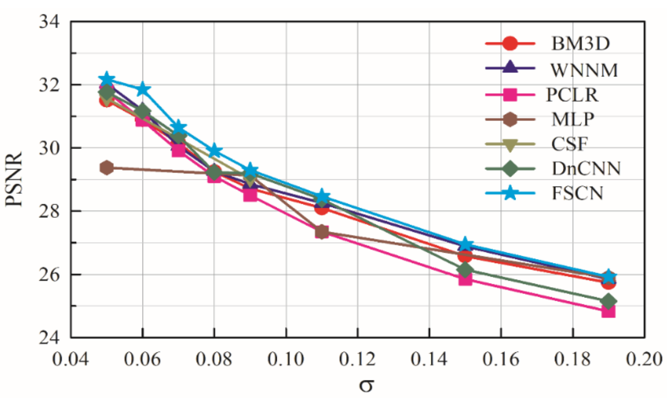
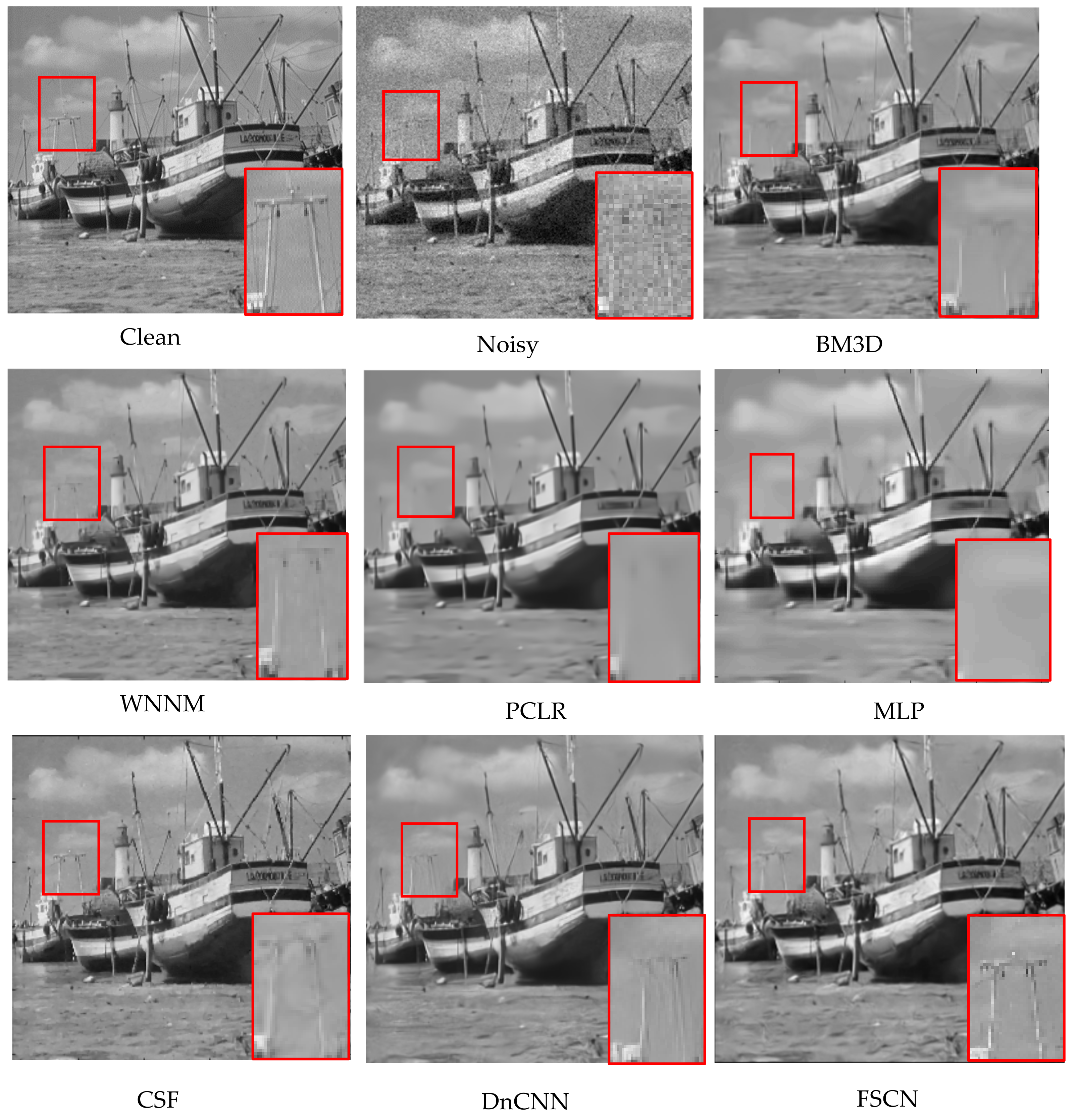
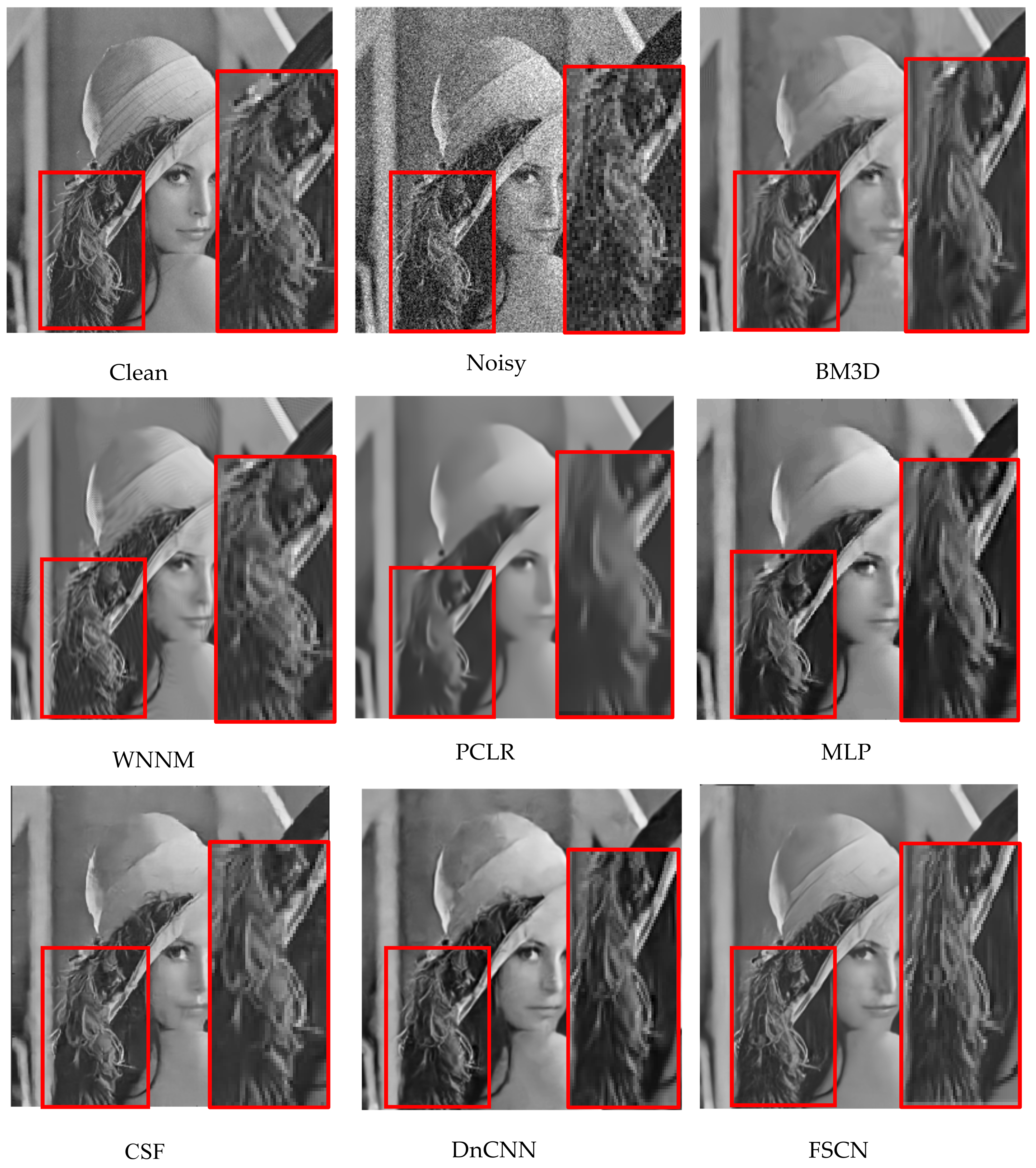
The learning procedure of all layers of the model is summarized in Algorithm 1. Ten common benchmark images [4,36,37] are used for testing to evaluate the proposed model. Given a test image, one can go forward through the network which shows superior performance compared to other existing methods. The focus here is to denoise the various corruption levels of noise and compare with other state-of-the-art algorithms.

Algorithm 1. Learning procedure of FSCN

Require: Training images, # layers L, # feature maps, # epochs E

forl = 1: L do %% Loop over layers

Initialize feature maps and filters

for epoch = 1: E do %% Epoch iteration

fori = 1: N do %% Loop over noisy images

Reconstruct input by calculating $y_i$ in Equation (4)

Calculate PSNR using f in Equation (10)

Compute reconstruction error by Equation (11)

Compute gradients by calculating g in Equation (6)

end for

end for

Update using ADAM optimizer by calculating ${\theta }_{i }$ in Equation (7)

end for

Output

3.3. Network Performance

Interpreting and understanding the behavior of deep neural networks remains one of the main challenges in deep learning. It is necessary to compare it with other known networks to understand new subjects and to interpret. From this perspective, comparative study enables determining the performance of various networks in terms of PSNR.

In this section, we compare variations of the CNN architecture based on the patterns of layers. The combination of convolution and deconvolution networks contains 15 layers [29,38] but there is no conclusive evidence to show which network performs better both quantitatively and qualitatively. To our knowledge, very few have used batch normalization for FCN-based image denoising.

We have classified existing networks into four different models and compared them with our proposed network. A series of experiments were conducted to analyze the results quantitatively using PSNR values. Experiments were performed on a Kaggle dataset with 256 × 256 resolution for seven different architectures with monochrome images. The dataset contained clean and noiseless images, and therefore, a noise process was integrated into the training procedure. The architectures were categorized into different models as shown in

Table 1. Network Performance.

Sl.no	Model	Architecture	PSNR
1	C	CCCCC CCCCC	31.51
2	D	DDDDD DDDDD	32.00
3	BN	DBDBD BDBDB	30.14
4		CBCBC BCBCB	30.31
5	CD	CCCCC DDDDD	32.03
6		DDDDD CCCCC	31.68
7		CDCDC DCDCD	32.70

. The 8-bit integer intensity values of the dataset (values from 0 to 255) were normalized to 1 for faster convergence, and an Adam optimizer was adopted for all architectures.

In the Convolution (C) network model, the image denoising task is formulated as a learning problem to train the convolution network. The convolution network acts as good feature extractor by which the goal of denoising is accomplished. However, some details in the denoised image are absent. In the Deconvolution (D) network model, the network provides a framework that permits the unsupervised construction of hierarchical image representations. Using the same parameters for learning each layer, the deconvolutional network can automatically extract rich features while denoising the image. This network suppresses noisy activations, makes blurry images sharper, and captures details in an image. The batch normalization (BN) model helps to overcome the internal covariate shift problem but the network faces the serious issue of overfitting and makes large oscillations after few epochs for a small learning rate (η = 0.01). Poor results demonstrate that this architecture is inefficient for denoising compared with other architectures.

The CD network model is composed of convolution and deconvolution layers. Two different architectures [((CCCCC DDDDD), (DDDDD CCCCC))] are experimented with in the CD network model. These architectures have been proposed for semantic segmentation [29,38] comprising 13 layers with pooling and unpooling operations. This architecture is emulated in our experiments for denoising with different numbers of layers, and their results are tabulated. It is evident that these architectures give better results compared to other architectures. However, loss of details while denoising the heavily corrupted images remains a major issue.

Therefore, we proposed a new architecture (CDCDC DCDCD) and performed similar experiments. The proposed architecture not only exhibited better PSNR values but also recovered images with subtle loss of details and by eliminating the corruptions.

3.4. Model Visualization

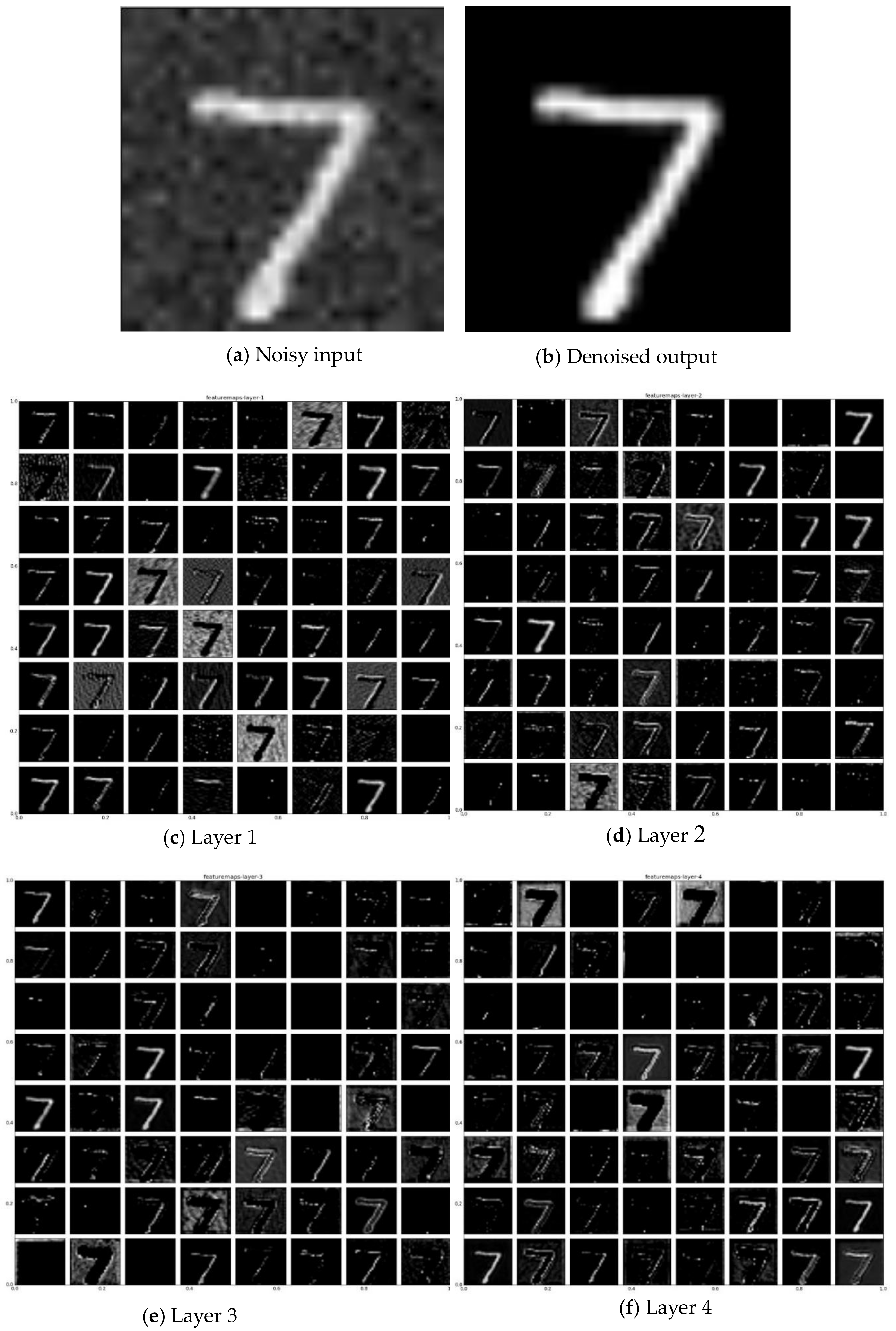
Visualizing outputs of each layer of a network can provide a good understanding of its behavior. The proposed FSCN model has demonstrated better denoising compared with other architectures. For a clear understanding of the superior performance, a visualization technique is employed to give insight into the function of intermediate feature layers. In Figure 3, we visualize the filters of the proposed model by taking each feature map separately. For visualization of the proposed architecture, the MNIST dataset with 28 × 28 image resolution is used. Each layer consists of (i) convolution of the previous layer output (or, the noisy image input as shown in Figure 3a in the case of the first layer) with a set of filters and (ii) passing the responses through ReLu. The top–down nature of the model makes it easy to inspect what it has learned. The parameters in the network are trained and updated via Adam.

In Layer 1, convolution layer extracts the overall feature from the noisy image input while reducing the noise. The less denoised image output is then fed as an input to the next deconvolution layer (Layer 2) which captures the overall shape of the image suppressing the noisy activations. The same process is continued until the image is denoised completely. Layers 1, 3, 5, 7, 9 (Figure 3c,e,g,i,k) show the feature maps after the convolution operation is applied to the noisy image. It is clear that the convolution operation acts as a useful feature extractor which encodes the primary components while eliminating corruptions.

Contrary to convolutional layers, which connect multiple input activations within a filter window to a single activation, deconvolutional layers associate a single input activation with multiple outputs. The learned filters in deconvolutional layers correspond to bases which reconstruct the shape of an input object. The deconvolutional layers are used to capture the different level of shape details. The filters in the lower layers tend to capture the overall shape of an object while the fine details are encoded in the filters of the higher layers. Layers 2, 4, 6, 8, 10 (Figure 3d,f,h,j,l) reveal that the deconvolutional layers decode the image abstraction from the convolutional layers to recover the details in the image. They also suppress noisy activations and make blurry images sharper. For each layer, it is apparent that the weights are not interpretable but are still smooth and well formed, with noisy patterns absent. Although all the layers share a similar form, they contribute different operations throughout the network. It gives some intuition for designing an end-to-end network in image processing. Well-trained networks display nice and smooth filters without any noisy patterns. Noisy patterns can be an indicator of a network that has not been trained for long enough or possibly may have led to overfitting. Therefore, it is evident that the image features are extracted by the layers and recovered efficiently in the intermediate layers.

4. Experimental Results

In this section, the experimental results of the FSCN model using different network parameters are discussed, and the image denoising is evaluated by calculating PSNR values and comparing with other few existing state-of-the-art methods. For training, 20,000 images from the Kaggle dataset with 256 × 256 resolution are used.

4.1. Network Parameter Setting

Although deeper networks tend to achieve better image restoration performance, problems related to different parameters still need to be investigated. A set of experiments is carried out with different network parameters: (a) filter number, (b) filter size, and (c) depth of the layers.

Filters act as feature detectors and the significance of the number of feature detectors is related to the number of features that the network can potentially learn. Each filter generates a feature map that allows the network to learn the explanatory factors within the image. Filter numbers 8, 16, 32, and 64 with fixed filter size 3 × 3 were chosen and the corresponding PSNR values were recorded on the validation set during training as shown in Figure 4. The figure shows that the filter number 64 achieved the best result in terms of PSNR values. However, a smaller number of filters is preferred for fast testing and suitable filter size has to be chosen to identify key features in the image. This helps to find the key features (edges, lines, shape, etc.) when convolved with appropriate kernels. Therefore, filter number 64 was chosen to study the PSNR output as a function of different filter size.

Large filter size may result in large receptive fields but this renders the networks more difficult to train and converge to a poor optimum. Using a large filter size inevitably increases the complexity, overlooks the features, and possibly skips the essential details in the image. On the other hand, small filters are favored for high-level tasks [35] and beneficial for convergence in complex mappings. Thus, it is important to choose the most suitable size of the filter. Filter sizes 2 × 2, 3 × 3, 4 × 4, and 5 × 5 were chosen for our experiment. Figure 5 shows the PSNR values on the validation set while training. It is observed that the filter size 3 × 3 gave the optimum result for the given filter number 64, whereas the PSNR values drastically decreased for higher-sized filters.

Experiments were also conducted for different depths of layers including 4, 6, 8, 10, 12, and 14, and PSNR values were recorded for validation. Figure 6 reveals that the performance increased gradually from layers 4 to 10 and began to decrease thereafter. Surprisingly, the PSNR dropped abruptly for a network with 14 layers and no information was recovered. Therefore, the 14-layer model was trained with filter number 32, filter size 3 × 3. The values obtained were still lower than values with the 10-layer model. Therefore, it is evident that a mere increase in layers without changing the parameters would actually degrade the performance. The reason for performance degradation may be due to the loss or corruption of image details with more convolution layers.

Deeper networks in image restoration tasks tend to easily suffer from performance degradation due to gradient vanishing and become much harder to train. This is one of the common problems faced by researchers in neural networks [39]. The average PSNR values tested on the standard 10 images for different depth layers as shown in Figure 7 clearly indicates that the 10-layer model achieved better performance. Therefore, in all our experiments, the 10-layer model was used with filter number 64, filter size 3 × 3, with an Adam optimizer.

4.2. Comparative Analysis of Algorithm

The results of the proposed FSCN method were compared with three nonlocal, similarity-based methods (i.e., BM3D [2], WNNM [11], and PCLR [37]), and three discriminative training-based methods (MLP [13], CSF [27], and DnCNN [28]). The source codes were downloaded from the authors’ websites and tested on the images with their default parameter settings. Ten common benchmark images were used for testing. A detailed comparison was made to evaluate the proposed model against the above competing algorithms on the standard test set.

4.2.1. Quantitative Evaluation

The average PSNR results of different methods on AWG noise with σ = 0.09 are shown in Figure 8. It can be seen that the proposed FSCN model yielded the highest PSNR on most of the images. The proposed model outperformed the competing methods by 0.4 dB to 0.8 dB on most of the images and failed to achieve best results only on two images, “Barbara” and “fingerprint”, which were dominated by repetitive structures and contained many regular structures. This result is consistent with the findings in [28,39]: nonlocal, means-based methods are usually better on images with repetitive and regular structures, whereas discriminative training-based methods generally produce better results on images with irregular textures. This is reasonable because images with regular and repetitive structures meet well with nonlocal similarity prior; conversely, images with irregular structures would weaken the advantages of such specific prior, thus leading to poor results.

The proposed model was also evaluated for varied noise levels (0.05–0.19) and produced best results on 8 out of the 10 test images. Figure 9 presents the average PSNR results of different denoising methods with respect to various noise levels. It is worth noticing that the proposed architecture gave a higher average PSNR value compared to WNNM, which is the best method known so far. From the above results and discussion, it is obvious that the combination of 10-layer convolutional and deconvolutional network achieves better results than previously known state-of-the-art methods in terms of denoising. The main reason for this superior performance of the FSCN model could be attributed to the sequence of convolution and deconvolution layers built in our architecture. Even the minute loss of details of the image contents were recovered due to the unique combination of layers.

4.2.2. Visual Quality Evaluation

Visual results of different methods are illustrated in Figure 10 and Figure 11. Some details of the clean images and the recovered images by different methods are highlighted for clarity. It can be seen that all other models tended to produce oversmoothed edges and textures compared to the FSCN model as shown in Figure 10. It is seen that the proposed FSCN model could well reconstruct the tiny masts of the boat, while the masts almost disappeared in the images reconstructed by other methods. Similarly, the proposed method outperformed other denoising algorithms on images with smooth surfaces and nonregular structures as shown in Figure 11. It is discernible that the proposed network obtained visually smooth results compared to other methods while retaining even the smallest details. It still tends to oversmooth image details and cause ringing artifacts.

4.2.3. Running Time

In addition to visual quality, another important aspect in the image restoration process is the testing speed with respect to image resolution. Figure 12 lists the running times of different algorithms for denoising gray images of sizes 128 × 128 and 256 × 256 with noise level 0.09. Unlike CSF and DnCNN algorithms, the running time for the proposed model remained consistent irrespective of the image resolution. It is highly efficient such that it can denoise an image of size 256 × 256 in just 0.2 s. Therefore, taking denoising performance and flexibility into consideration, the proposed model is competitive for practical applications as it achieves very appealing computational efficiency. The evaluation was performed in MATLAB(R2015b) environment on a computer with a dual-core Intel(R) Xeon(R) CPU E5-2650LV3 @1.80 GHZ, 32 GB of RAM for BM3D, WNNM, PCLR, and MLP and an NVidia Titan X GPU was used for CSF, DNCNN, and FSCN algorithms. The NVidia cuDNN-v5.1 deep learning library was used to accelerate the computation of the FSCN model. However, different execution environments did not influence the finding that the deep-learning-based approach has the performance advantage for the restoration stage of image denoising.

5. Conclusions

Convolutional networks have played an important role in the history of deep learning. In this work, convolution and deconvolution layers are alternatively combined to extract the primary image content and recover details. The proposed model was tested for various filter numbers, filter size, optimizers, and depth of layers. It was also compared with other existing state-of-the-art methods. The results on standard images with AWGN demonstrated that the proposed model not only led to visual PSNR improvements but also preserved the image local structure more effectively. The superior denoising and visual results prove that the proposed model can recover the image details efficiently compared to other methods. The running time comparisons showed that the FSCN model is fast and effective, suggesting it to be very practical for CNN-based denoising applications. The application of this model could also be envisioned for other tasks with appropriate tuning of hyperparameters.