Control of Flow around an Oscillating Plate for Lift Enhancement by Plasma Actuators

Featured Application

Micro air vehicles.

Abstract

During insect flight, a feathering motion of the wing’s controls vortex shedding for lift enhancement. In this study, in order to control the flow around a wing flapping with simplified sinusoidal motion, plasma actuators were introduced to simplify the complex feathering motion. In a wind tunnel, a smoke-wire method was enacted to visualize the flow fields around an oscillating plate with an attack angle of 4° in a uniform flow for the baseline and controlled cases. The actuator placed around the leading edge was found to suppress the flow separation on the top surface. Numerical simulations were performed to investigate the control effects on the fluctuating lift, where the control effects by the intermittently driven actuator were also predicted. The actuator installed on the top surface throughout the up-stroke motion was found to suppress vortex shedding from the trailing edge, which resulted in an 11% lift enhancement compared to the baseline case. In regard to the effects of the installation position, it was found that the actuator placed on the top surface was effective, compared to the cases for installation on the bottom surface or both surfaces.

1. Introduction

Recently, to better understand the dynamics of flying insects, the development of micro air vehicles (MAV) has been progressed. The MAVs, with a maximal dimension of 150 mm, normally operate in the Reynolds number regimes of 10⁴–10⁵ or lower, in which most flying animals fly [1] and the boundary layer tends to be laminar [2,3]. A number of MAV designs including fixed, rotary and flapping wings have been proposed [4,5,6,7]. The MAVs with fixed wings are capable of high-speed and efficient flight and the MAVs with a rotary wing are capable of hovering [7]. Compared with fixed-wing craft or rotorcraft, bio-inspired flapping-wing MAVs have more likely possibility to be scaled down in size [7].

The research on the bio-inspired MAVs have primarily focused on the wing shape of creatures [8] such as butterflies [9], beetles [10] and dragonflies [11,12]. Particularly, the dragonfly has high flight performance such as hovering, accelerating in almost any direction and precise maneuver at a high speed [12,13,14]. It is well known that dragonflies fly with simultaneous feathering and flapping motions of their wings [15]. For the dragonflies in flight, the flow is separated on the top surface of the wing, when the wings are moved in down-stroke motion. At this time, lift force is generated by the negative pressure on the top surface due to the separation vortices. In addition, lift is generated during the up-stroke motion by the remaining vortices on the top surface, where the generation of vortices on the lower surface is suppressed by the feathering motion [16].

To develop a MAV that simulates the flight of dragonflies, a mechanism that combines both flapping and feathering motions is necessary. If the feathering motion of insects is able to be reproduced by combining simple vertical oscillations of wing and active flow control, it can provide new knowledge for MAVs.

There are various active fluid control techniques including suction and blowing [17,18,19,20], synthetic jets [21,22,23]. Recently, the research on the flow control by plasma actuators has been performed [24,25,26,27,28,29,30,31]. The plasma actuator is a structure composed of upper and lower electrodes and a dielectric layer, as shown in Figure 1. By applying an alternating voltage with the high amplitude and frequency between the two electrodes, plasma is generated between the electrodes. As a result, induced flow occurs from the upper electrode toward the lower one. Compared with other flow control techniques, the plasma actuator has two key advantages; with its simple structure, installation is easy and disturbances in flow caused by installation are minimal owed to the actuator’s thin structure and fast time response [24]. Singhal et al. [25] showed that the dynamic stall vortex can be suppressed with a sufficiently high excitation Strouhal number. Inasawa et al. [26] clarified that the suppression control of tonal noise generation at an airfoil trailing edge was conducted by using a flush-mounted plasma actuator for a NACA0012 airfoil at an angle of attack of 2°. Post et al. [27] found that the actuator controls the stall flow around a wing with pitching movement, where the time-average lift force increases.

The ultimate goal of this investigation is to effectively enhance lift force with a simple flapping wing by using a plasma actuator to control flow and replace the feathering motion of insects. To work towards this goal, wind tunnel experiments and numerical simulations were performed to clarify the control effects of the plasma actuator on the flow around an oscillating plate in a uniform flow.

In Section 2, the flow configuration, control parameters of the actuators, the experimental methods and the computational methodologies are explained. In Section 3, the computational validation on the control effects is discussed. In Section 4, the predicted control effects of the actuator on flow fields around the oscillating plate are presented. In Section 5, conclusions are summarized.

2. Method

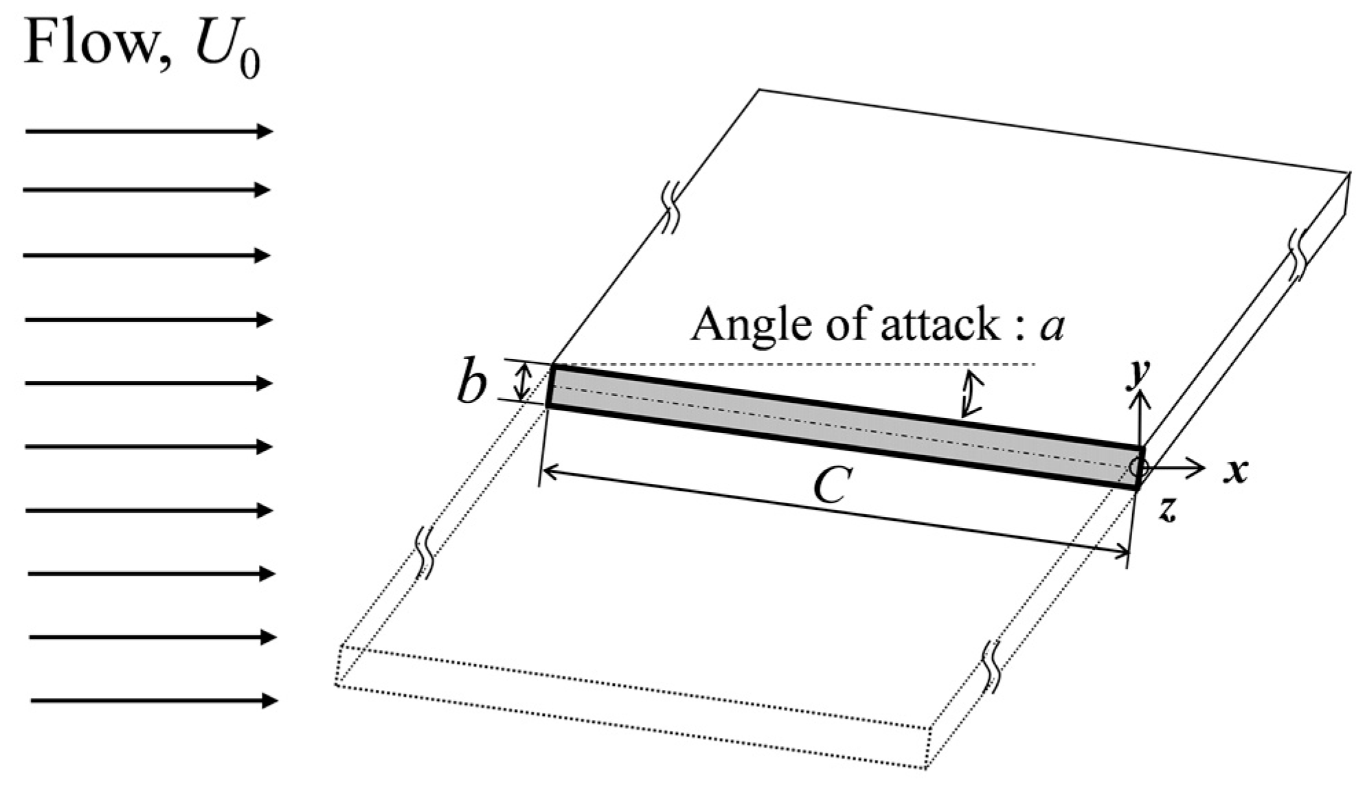
2.1. Flow Configurations

Figure 2 depicts the present configuration of the oscillating flat plate in the freestream. The plate is oscillated in the up-stroke and down-stroke directions with a constant attack angle of α = 4°. The origin of the coordinate system is located at the midpoint between the top and bottom downstream edges of the plate positioned at the center of the oscillation motion. The x, y axes are set to be the freestream and vertical directions, respectively. The z axis is set to be the span-wise direction. The ratio of the plate length to plate thickness is C/b = 15. The Reynolds number based on the plate thickness and the freestream velocity, U₀, is Re_b = 159. In the experiments, the freestream velocity U₀ was 1.2 m/s and the plate length C was 30 mm.

During the experiment, the plate was oscillated in a sinusoidal waveform and the oscillation frequency was f_oscib/U₀ = 0.01. Meanwhile, the amplitude was A/b = 0.7 and the vibration velocity was 2πf_osciA/U₀ = 0.044. In this study, the Reynolds number based on the plate cord length was Re_c = 2.4 × 10³ and reduced frequency [1] was k ≡ πf_osciC/U₀ = 0.47. For dragonflies, the flapping frequency is f_osci ≈ 30 Hz [12] and the chord length is C ≈ 10 mm [16]. Assuming that a dragonfly flies in an air current of 1–5 m/s, the Reynold number is Re_c = 0.7 – 3.3 × 10³ and the reduced frequency is k = 0.2–0.9. The present conditions of the Reynolds number and the reduced frequency are within these ranges.

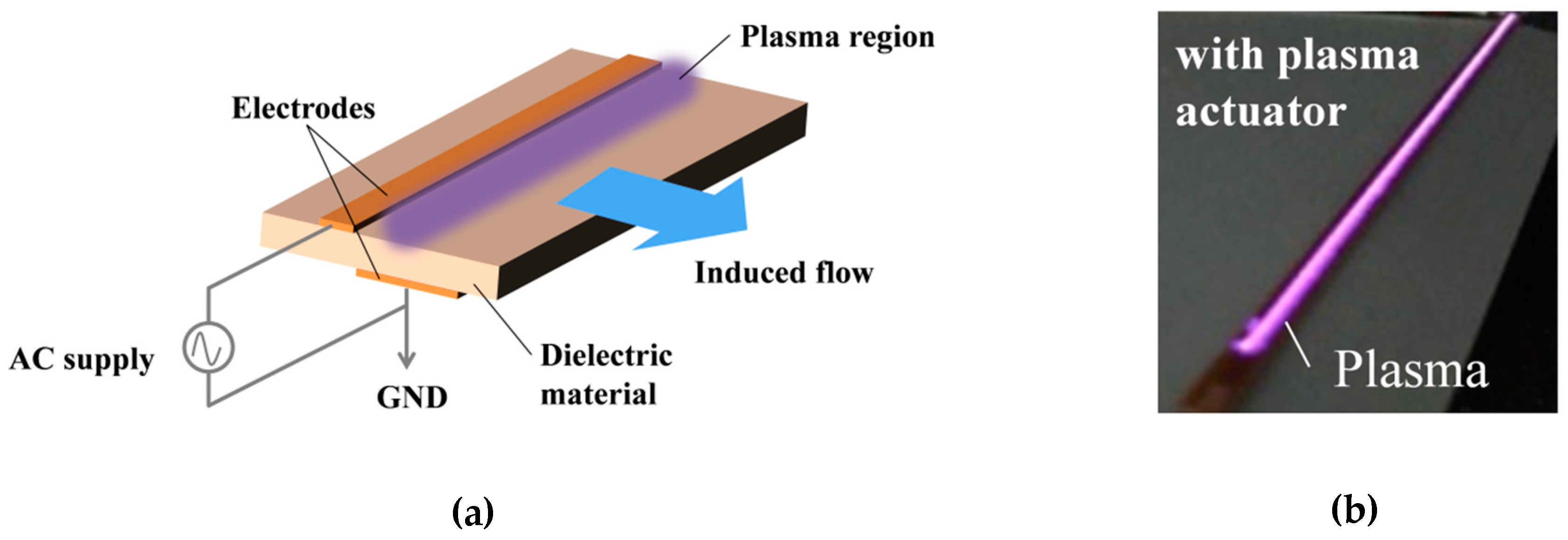
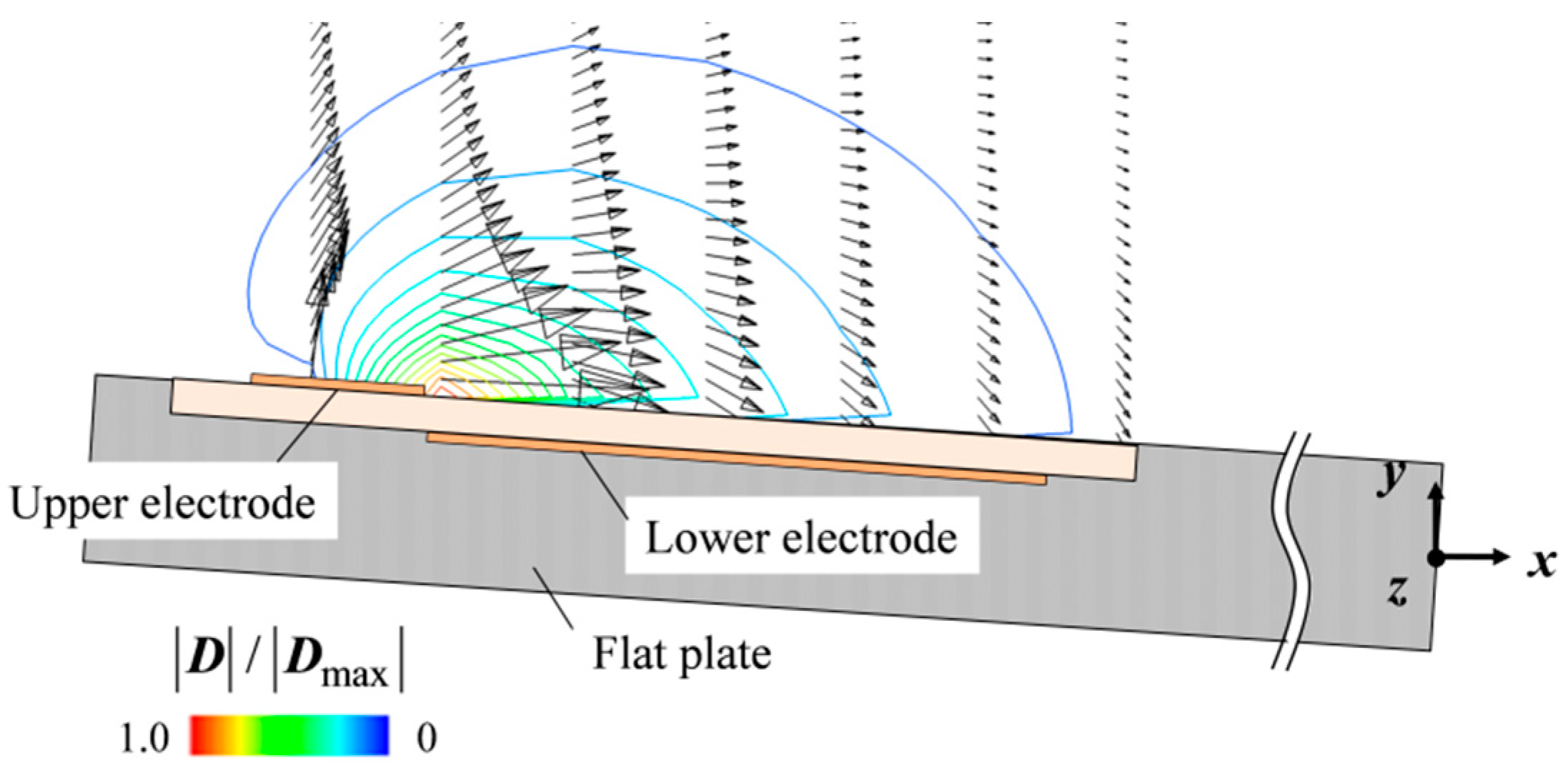
2.2. Configurations and Control Parameters of Plasma Actuator

Figure 3 illustrates the cross-section of the plasma actuator utilized in this study. To minimize the influence on the flow due to the protrusion of the actuator from the wall, a flush-mounted plasma actuator [24,26,31] was utilized. A copper foil with a thickness of 0.006b was used as the upper and lower electrodes and polyimide with a thickness of 0.2b was used as the dielectric layer. The alternating voltage with a peak-to-peak voltage of E_PA = 4.8 kV_p-p was applied with the frequency of f_PA = 4.2 kHz. The widths of the upper electrode and the lower electrode were 0.5b and 1.5b, respectively. The plasma actuator was installed 0.25b downstream from the upstream edge. In the previous paper [31], it has been confirmed that the actuator with these configurations suppressed the flow separation around the plate, where the control effects are shown in Section 3. It was found in the literature [24] that the flow control by the plasma actuator set near the separation point was effective for suppression of flow separation. However, the protrusion of the actuator could disturb the flow in itself by setting the actuator just at the leading edge because the shape of the leading edge of the flat plate affects the flow phenomena such as vortex shedding. Based on these considerations, the actuator was located at slightly downstream position from the upstream edge.

Also, to clarify the effects of installation surface on the control, the control effects were investigated with the actuators installed on the top surface, bottom surface and both surfaces, as shown in Figure 3.

To clarify the influence of the driving conditions of the actuator on the lift force, the control by the intermittently driven actuator with two changed parameters was investigated along with the continuous control. The first parameter is the ratio of time duration for driving the actuator to the oscillation period (driving ratio), R. The second parameter is the difference between the time to start driving the actuator and that for the bottom dead point of plate oscillation (time offset), t₀/T. These two parameters were changed as shown in Figure 4, where T is an oscillating period and t = 0 is the time for the bottom dead center of the oscillating motion. A driving ratio of 0% indicates that the plasma actuator is not driven, while a driving ratio of 100% indicates that the plasma actuator is continuously driven throughout the oscillation. The offset of 0.0 means that the actuator is driven from the time at which the up-stroke motion begins.

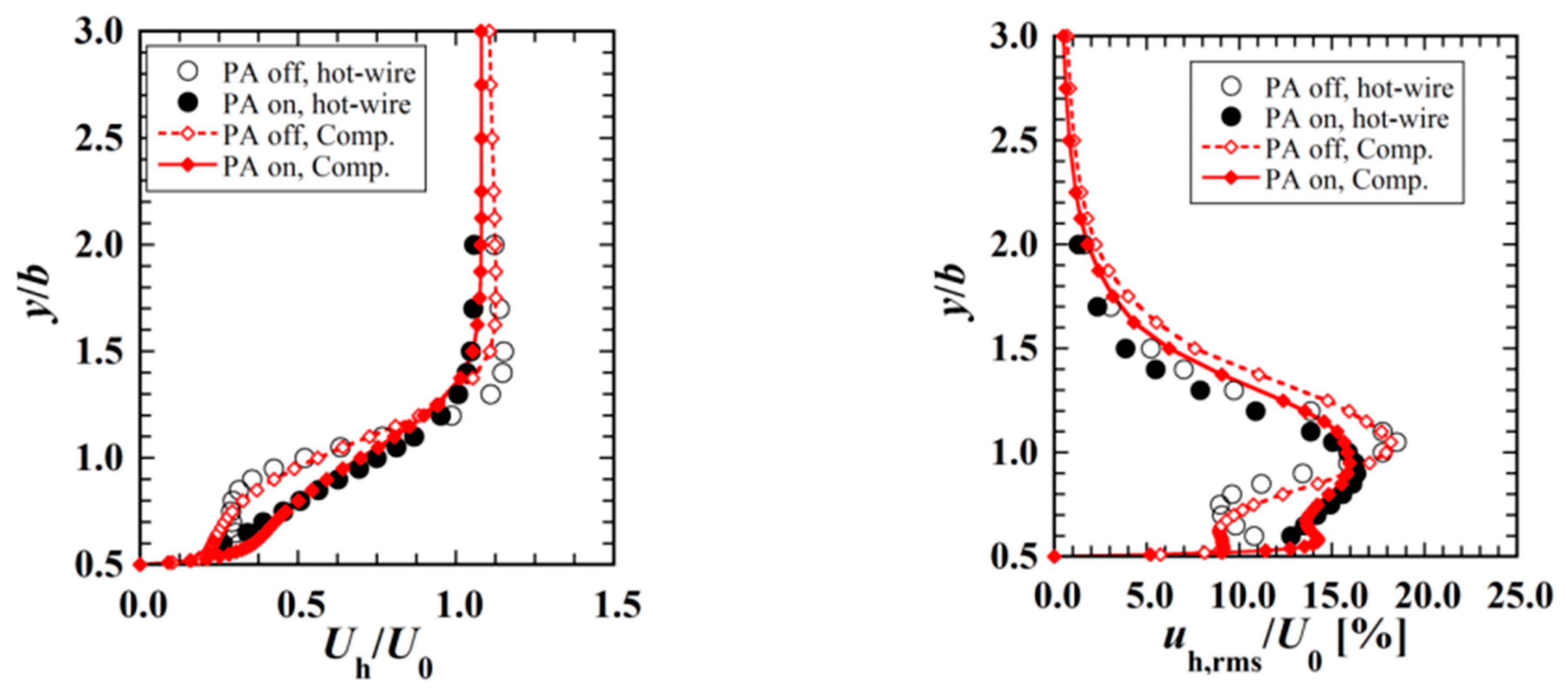
2.3. Experimental Methodologies

The experiments were conducted in a Göttingen-type small wind tunnel. The plate was placed in the open test section with a y-z square cross-section with the side length of H = 400 mm. The flat plate was located 0.25H downstream from the nozzle exit. The plate was oscillated by the link mechanism depicted in Figure 5. The wall effects of the wind tunnel were suppressed by utilizing an open test section and a sufficiently larger nozzle exit with a side length of 13.3C. The visualized flow in the experiment for the flow around a fixed plate (α = 4°) was compared with the predicted streamline as shown in Figure 6. The measured height of the separation bubble at the downstream point from the leading edge with the distance of 10b is 2.0b and the same as the value based on the predicted streamline in the simulation with sufficiently large height for the freestream region as shown in Figure 8. This result indicates that the wall effects in experiment are negligibly small. The linkage and motor of the link mechanism were set outside of the flow from the nozzle, where the spanwise length between the struts for the slide of the plate was 0.75H.

It was confirmed that the variation of the freestream velocity was within 0.04 m/s in all experimental conditions. The amplitude of displacement of plate oscillation was adjusted by the pictures by the camera with the accuracy of 0.1 mm and the variation of the amplitude during 30 s was 2.4%.

In order to visualize the flow field around the plate, a smoke-wire technique was utilized. In this setup, the flow field was illuminated by a green laser (1 mm thickness) and observed by a digital camera (Nikon D5200, NIKON CORPORATION, Tokyo, Japan) with an aperture value of 5.6, shutter speed of 1/400 s and ISO sensitivity of 3200. The plate was made of aluminum, where the surface was anodized in order to prevent the reflection of laser light. To seed the smoke, a pair of twisted nichrome wires with a diameter of 0.2 mm were covered with a mixture of liquid paraffin, glycerin and surfactant and heated to evaporate the mixture by a DC power supply (ZX-400LA, Takasago LTD., Kanagawa, Japan). A timer device (MSA Factory, Tokyo, Japan) was utilized to control the time for heating the wire.

2.4. Computational Methodologies

2.4.1. Governing Equations and Finite Difference Scheme

In this simulation, the three-dimensional Navier-Stokes equations along with the mass and energy conservation laws were solved using a six-order-accurate compact finite difference scheme (fourth-order-accuracy at the boundary) for both the inviscid and viscous flux vectors [32]. The time integration was explicitly performed with a third-order-accurate Runge-Kutta method. To reproduce a moving object, such as the oscillating plate, in a static rectangular computational grid, the volume penalization (VP) method [33,34] was utilized.

The external penalization term, V and the plasma actuator term, D, which is described in detail in Section 2.4.2, were added to the right-hand side of the governing equations of the three-dimensional Navier-Stokes equations as follows:

$${\mathit{Q}}_t+{\left({\mathit{F}}_x-{\mathit{G}}_x\right)}_x+{\left({\mathit{F}}_y-{\mathit{G}}_y\right)}_y+{\left({\mathit{F}}_z-{\mathit{G}}_z\right)}_z=\mathit{V}+\mathit{D},$$

(1)

where Q is the vector of the conservative variables, F are the inviscid flux vectors, G are the viscous flux vectors, V is the penalization term as follows:

$$\mathit{Q}=\left(\begin{array}{c}\rho \\ \begin{array}{c}\rho u\\ \rho v\\ \rho w\end{array}\\ e\end{array}\right),{\mathit{F}}_x=\left(\begin{array}{c}\rho u\\ \begin{array}{c}\rho uu+p\\ \rho vu\\ \rho wu\end{array}\\ \left(e+p\right)u\end{array}\right),{\mathit{F}}_y=\left(\begin{array}{c}\rho v\\ \begin{array}{c}\rho uv\\ \rho vv+p\\ \rho wv\end{array}\\ \left(e+p\right)v\end{array}\right),{\mathit{F}}_z=\left(\begin{array}{c}\rho w\\ \begin{array}{c}\rho uw\\ \rho vw\\ \rho ww+p\end{array}\\ \left(e+p\right)w\end{array}\right),$$

(2)

$${\mathit{G}}_x=\left(\begin{array}{c}0\\ \begin{array}{c}{\tau }_{xx}\\ {\tau }_{yx}\\ {\tau }_{zx}\end{array}\\ G_{x5}\end{array}\right),{\mathit{G}}_y=\left(\begin{array}{c}0\\ \begin{array}{c}{\tau }_{xy}\\ {\tau }_{yy}\\ {\tau }_{zy}\end{array}\\ G_{y5}\end{array}\right),{\mathit{G}}_z=\left(\begin{array}{c}0\\ \begin{array}{c}{\tau }_{xz}\\ {\tau }_{yz}\\ {\tau }_{zz}\end{array}\\ G_{z5}\end{array}\right),G_{i5}=u_j{\tau }_{ij}$$

(3)

$$\mathit{V}=-\left(\frac{1}{\varphi }-1\right)\chi \left(\begin{array}{c}\partial \rho u_i/\partial x_i\\ 0\\ 0\\ 0\\ 0\end{array}\right),$$

(4)

$$\phi =0.25,$$

(5)

$$\chi =\{\begin{array}{c}\min \left(1,\left|d/\Delta y\right|\right)\\ 0\end{array}\begin{array}{c}\left(\mathrm{inside}\mathrm{object}\right)\\ \left(\mathrm{outside}\mathrm{object}\right)\end{array},$$

(6)

where ρ is the density of the fluid, u, v and w are the velocities in each direction, p is the pressure, e is the total energy per unit volume, τ_ij is the viscous stress tensor.

The variable χ was the mask function, where χ was set to be zero outside the object and 1 inside the object, excepting the region near the surface of the oscillating plate. To prevent the generation of artificial pressure waves, the mask function was smoothly changed between the inside and outside of the object by the ratio of the distance from the surface of the object, d and the grid resolution, Δy, in the object near the surface (d/Δy < 1). In the objects, the velocity was set to zero and the constant ambient temperature (293 K) was given. The coefficient, φ, which is defined as the porosity of the porous medium in the original VP method [34], was here determined as 0.25 considering the computational stability. It has been confirmed that the flow field around an oscillating plate was correctly predicted by the present methodologies [35].

2.4.2. Body Force Generated by Plasma Actuator

The distributions of the body force in the x-y cross-section were computed by the distributions of the plasma charge, ρ_c and potential, $\phi$, which were predicted by the electric computational methodologies proposed by Suzen et al. [36].

Since the electrodes of the plasma actuator are uniform in the span-wise direction in the experiment, the two-dimensional body force was also given in the simulation. Referring to previous research [30], the expressions for the given body-force vector are as follows:

$$\mathit{D}=\left(\begin{array}{c}0\\ C\left(t\right){\rho }_c\left(-\nabla {\phi }_k\right)\\ C\left(t\right){\rho }_c\left(-\nabla {\phi }_k\right)·u_k\end{array}\right),$$

(7)

$$C\left(t\right)=A{\sin }^2\left(2\pi f_{\mathrm{pa}}t\right),$$

(8)

$$A=1\left(\sin \left(2\pi f_{\mathrm{pa}}t\right)\le 0\right),-0.4\left(\sin \left(2\pi f_{\mathrm{pa}}t\right)>0\right),$$

(9)

The variable C(t) was introduced to reproduce the effects of the discharge occurring twice during one cycle of the plasma actuator’s applied frequency [37]. Also, the variable A was introduced to reproduce the change of the induced flow with the positive or negative voltage of the applied alternating voltage, which was observed in experiments by Forte et al. [38]. It has been confirmed that it is possible to correctly predict the induced flow due to the plasma actuator by the present methodologies [30,31].

The predicted distributions of the body force are shown in Figure 7, where the maximum value of the body force in the space is defined as D_max/(ρU₀²/b) = 341, which was adjusted referring to visualized flow fields. This figure expresses that the stream-wise body force is generated particularly in the downstream of the upper electrode. The computational region for applying this body force was moved along with the oscillation of the plate with the plasma actuator.

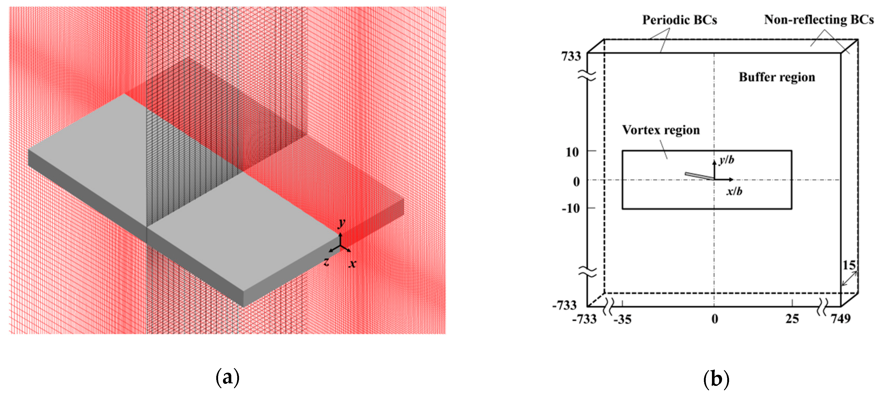
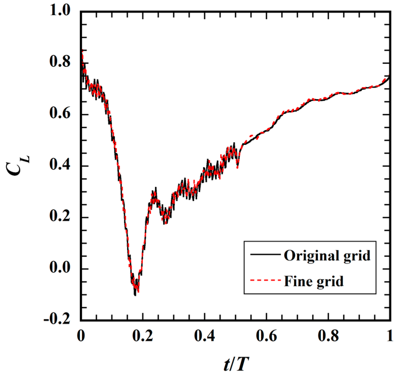
2.4.3. Computational Grids

Figure 8 displays the computational grids and domain for the flow around the oscillating plate. The computational regions are composed of two regions: the vortex and buffer regions. In the vortex region, the grid resolutions in the region for the passage of the oscillating plate are constantly Δx_min/b and Δy_min/b = 0.05, which are sufficient for the above-mentioned oscillation amplitude of A/b = 0.7. Also, 34 grid points were approximately utilized for the height of the separation bubble (≈ 2b) around the leading edge. The growth factor of the adjacent grid resolution was adjusted to be within 1.2 in the entire computational region for the computational accuracy.

In the vortex region, to solve the fine vortices of the wake of the flat plate with the extent of L_v/b = 1.0, the maximum grid spacing was set to be Δ_max/b = 0.1. Also, the sufficiently large buffer region was set outside the vortex region, where the grid resolution is smoothly stretched from within the vortex region to dissipate the pressure waves near the artificial boundaries to minimize the reflection on the boundary. The span-wise extent of the computational domain was L_s/b = 15. In the span-wise direction, 31 grid points were used, while the predicted flow was approximately two-dimensional due to the low Reynolds number of the flow as presented in Section 4.1. The total grids contain approximately 9.8 × 10⁶ grid points.

To investigate the effects of the grid resolution on the computational results, the simulation with finer grid resolution was performed, where the grid resolution in all directions was set to be smaller with the factor of 0.67 compared with the original resolution. Figure 9 shows the predicted time variation of the lift coefficient for the control condition of t₀/T = 0.0 and R = 50% with the original and finer grids. As shown in this figure, the effects of changing the grid on the results are negligibly small. This indicates that the present grid is sufficiently fine to predict the flow field around the oscillating plate.

2.4.4. Boundary Conditions and Initial Conditions

Figure 8 also shows the boundary conditions. In the span-wise direction, periodic boundary conditions were adopted. In other boundaries, non-reflecting boundary conditions were utilized to prevent reflections of the pressure waves on the artificial boundaries.

The freestream velocity and pressure were given in the entire computational region except the region of the flat plate as the initial condition. After the computation was conducted during nine oscillation periods for flow development, the variation of the lift coefficient and flow fields such as streamline were sampled, which are presented in this paper.

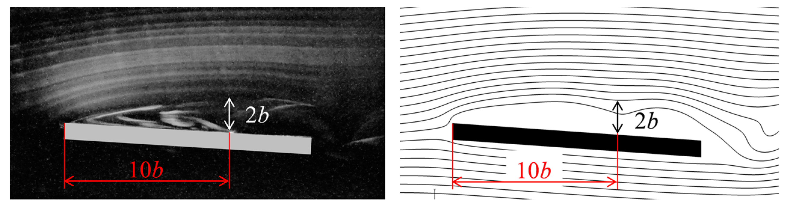
3. Comparison of the Visualized and Predicted Flow Fields

Figure 10 shows the visualized flow by the smoke-wire method and the predicted streamline around the oscillating plate with and without control by the actuator at t/T = 0.0, 0.25, 0.50 and 0.75. To discuss the flow fields, a simple grid with the lattice spacing of 2b was set in both the figures of the visualized photograph and the predicted streamline. The actuator was installed only on the top surface and continuously driven in the case with control (R = 100%).

As shown in Figure 10, the flow separation from the upstream edge occurs on the top surface except at t/T = 0.5 (top dead center) in the baseline case for both the measured and predicted results. A laminar flow separation bubble is observed at t/T = 0.0, where the height of the bubble is 2.1b and 2.0b at the downstream point from the leading edge with distance of 10b for the measured and computational results, respectively. In the visualization experiment, the height of separation bubble was averaged for ten photographs and the variation was about 6%. Also, the height of separation bubble at the above-mentioned point at t/T = 0.25 is 2.6b and 2.4b for the measured and computational results, respectively. Also, the flow reattachment occurs at the above-mentioned point at t/T = 0.75 for both the measured and predicted results. These results present that the predicted flow fields at each time are in agreement with those visualized for the baseline case. In the case with control, the flow separation around the leading edge is almost suppressed, while the flow is slightly separated around the center of the plate, particularly at t/T = 0.25. These flow behaviors were observed in both the measured and predicted flow fields.

In the previous paper from the same group [31], the predicted control effects on the flow around a fixed plate (α = 0°) by the plasma actuator were compared with those measured by a hot-wire anemometer. In this study, the actuator with the same configurations as that in the present paper was located at the same position with the distance of 0.25b from the leading edge. The computational model of the body force by the actuator was also the same as that in the present computations. Figure 11 shows the predicted and measured vertical distributions of the mean velocity and turbulence intensity with and without the control by the actuator at the downstream position from the leading edge with the distance of 4.5b. Both the predicted and measured results show the suppression of the flow separation by the control [31]. Also, both the predicted distributions with and without control are in good agreement with those measured.

These results suggest that the present computations correctly capture the flow fields around the oscillating plate, including the control effects of the plasma actuator.

4. Results and Discussion

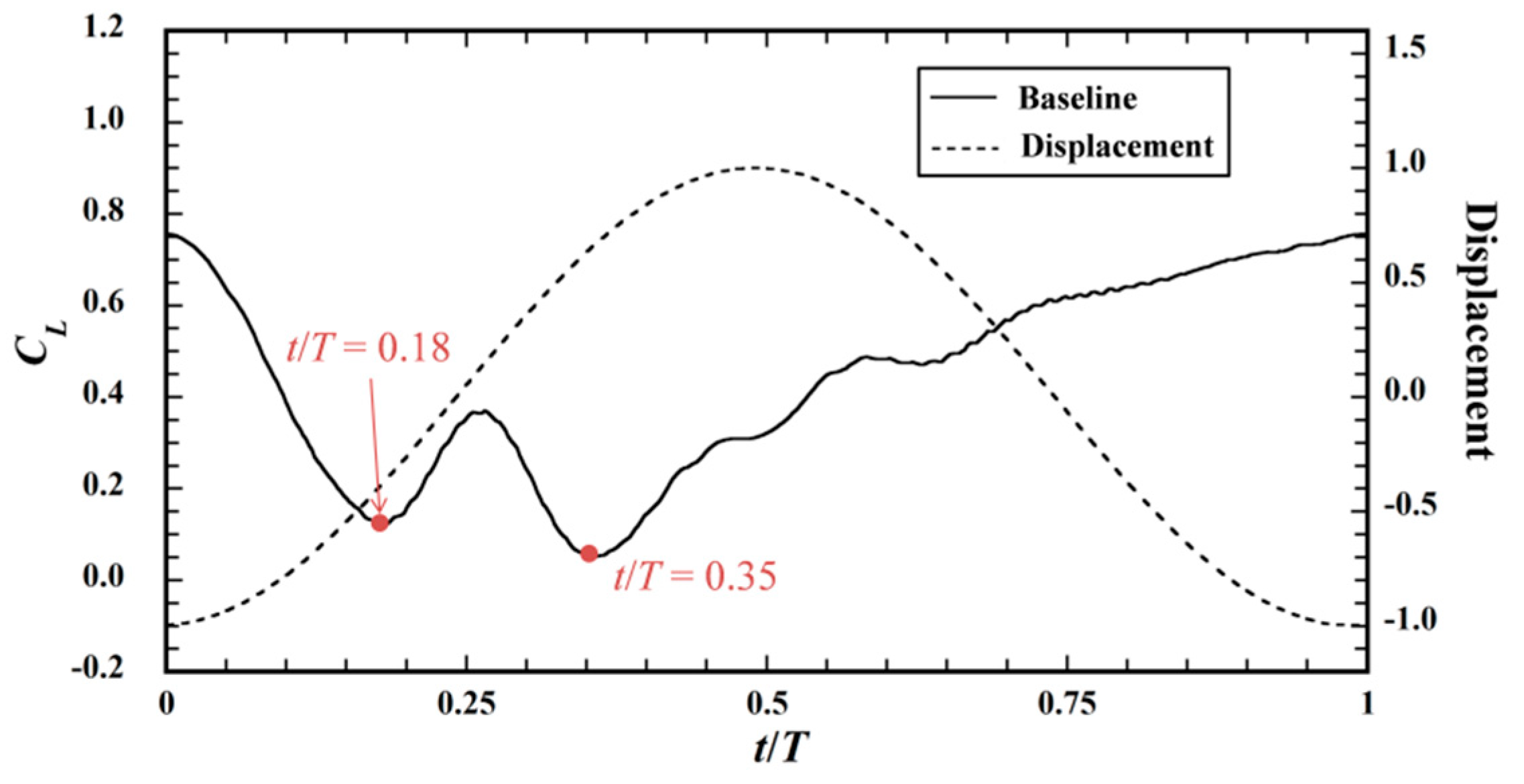
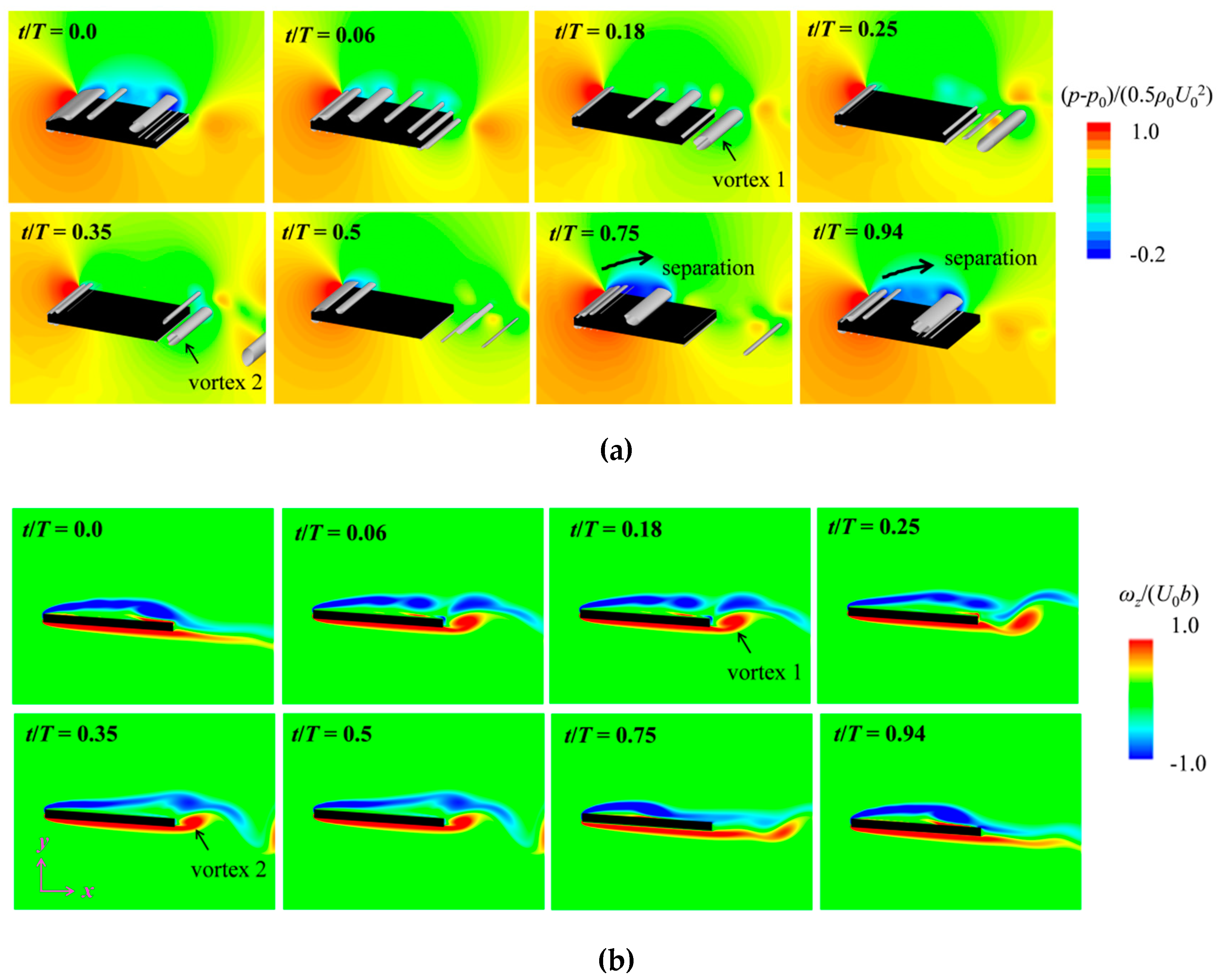
4.1. Lift Fluctuation in Baseline Flow

In this section, the relationship between the lift fluctuations and the flow field are discussed for the baseline flow. The lift force exerted on the plate periodically fluctuates along the oscillation motion. Figure 12 demonstrates the time fluctuations of the lift coefficient in an oscillation period in the baseline case, where the dashed line indicates the displacement of the flat plate without the dimension of amplitude. These fluctuations are related to the vortices and pressure field around the plate. Figure 13a depicts the iso-surfaces of the second invariant of the velocity gradient tensor (vortices) with the contours of the pressure, subtracting ambient pressure, p₀. As shown in the figures, the vortical structures are two-dimensional in the span-wise direction, where the pressure distributions are also uniform in the span-wise direction. In an actual MAV, the vortical structures around the flapping wing possibly become three-dimensional due to the influence of the tip of the wing or three-dimensional flapping. In the present simulation, the flapping was two-dimensional up-and-down movement and the tip of the wing was not considered. Along with the low-Reynolds-number conditions, this possibly leads to the occurrence of the two-dimensional vortices. Also, it is noted that two-dimensional vortices were also confirmed in the above-mentioned computational results with finer spanwise grid resolution width with the factor of 0.67 compared with the original resolution. Also, Figure 13b illustrates the contours of the vorticity around the oscillating plate.

Figure 12 expresses that the lift coefficient decreases with time as t/T = 0.0–0.18 in the up-stroke motion. As shown in Figure 13a, the large separation vortices with a low-pressure region generated in the down-stroke motion (t/T = 0.94) become weaker on the top surface. As a result, the pressure on the top surface increases in the up-stroke motion, which subsequently decreases lift.

The lift coefficient increases and decreases again between t/T = 0.18–0.35 as shown in Figure 12. The low lift coefficients at t/T = 0.18 and 0.35 are due to the vortex shedding from the trailing edge on the bottom surface (vortex 1 and vortex 2 shown in Figure 13). This phenomenon decreases the pressure on the bottom surface and consequently the lift. At t/T = 0.25, the flow is largely separated on the top surface as displayed in Figure 10 and the vortex shed from the bottom surface at t/T = 0.18 (vortex 1) is convected far from the plate into the downstream as shown in Figure 13b. As a result, the pressure of the top and bottom surfaces is decreased and increased, respectively, which causes lift to increase.

In the down-stroke motion (t/T = 0.5–1.0), the lift coefficient gradually increases from t/T = 0.5 to 1.0. This is because a separation vortex becomes larger on the top surface and the pressure on the top surface becomes lower as illustrated in Figure 13a.

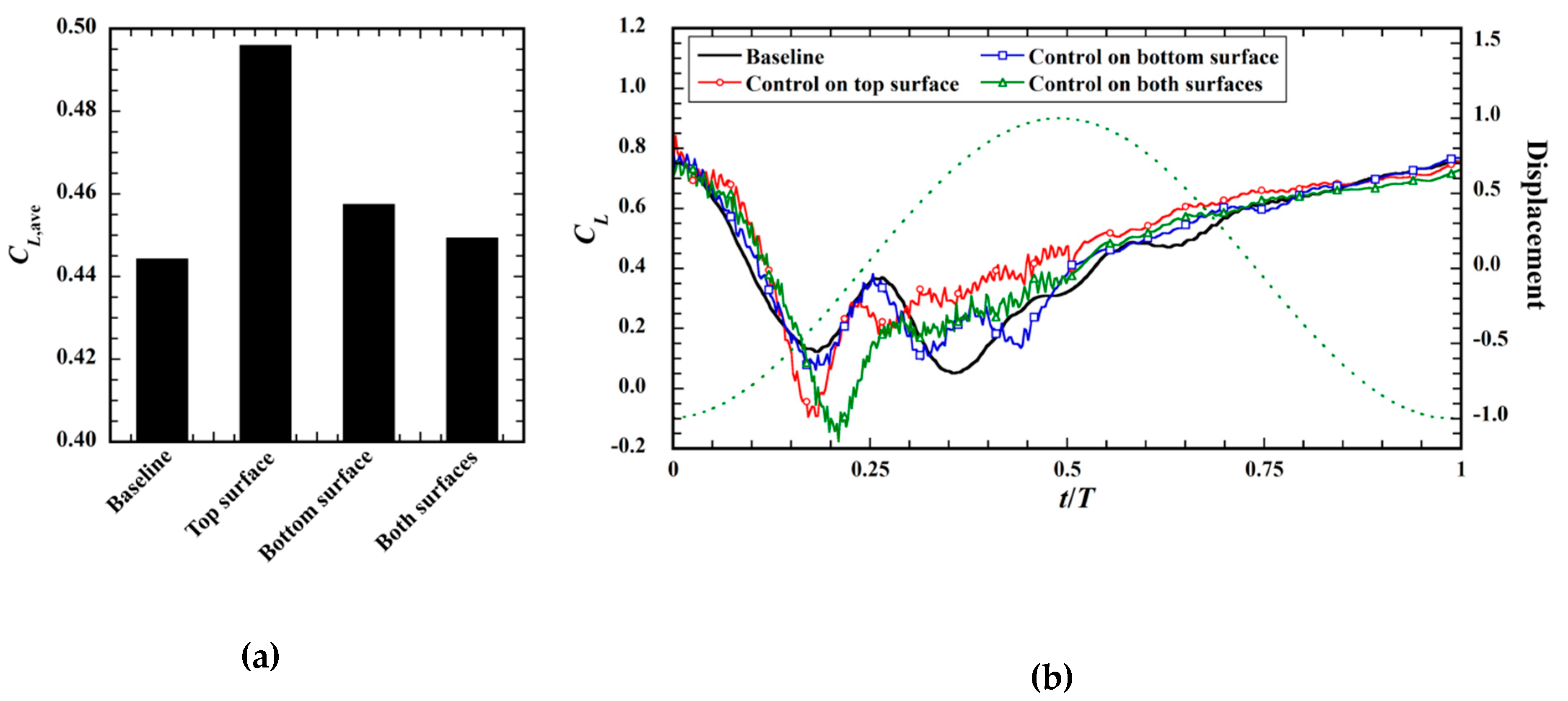
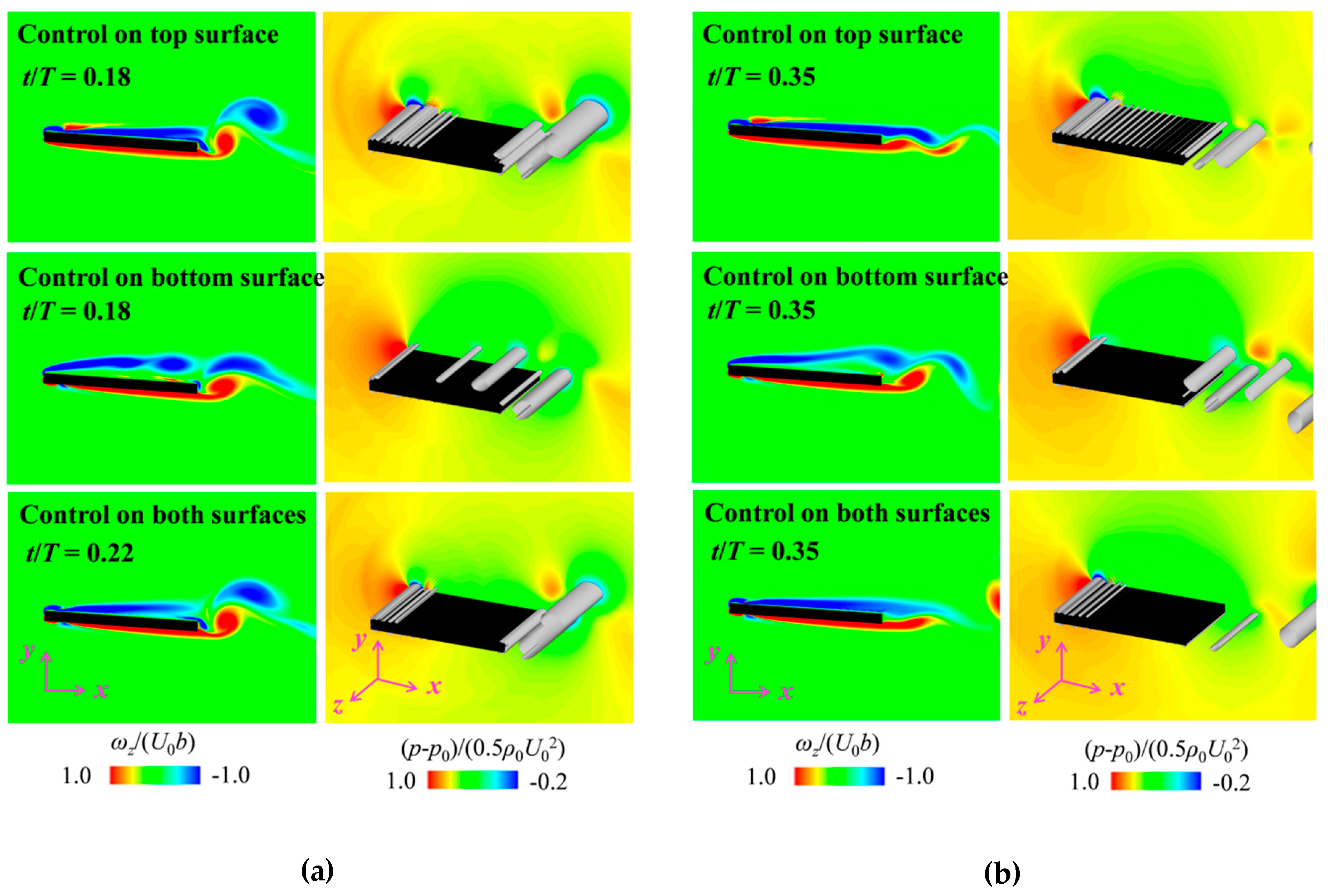
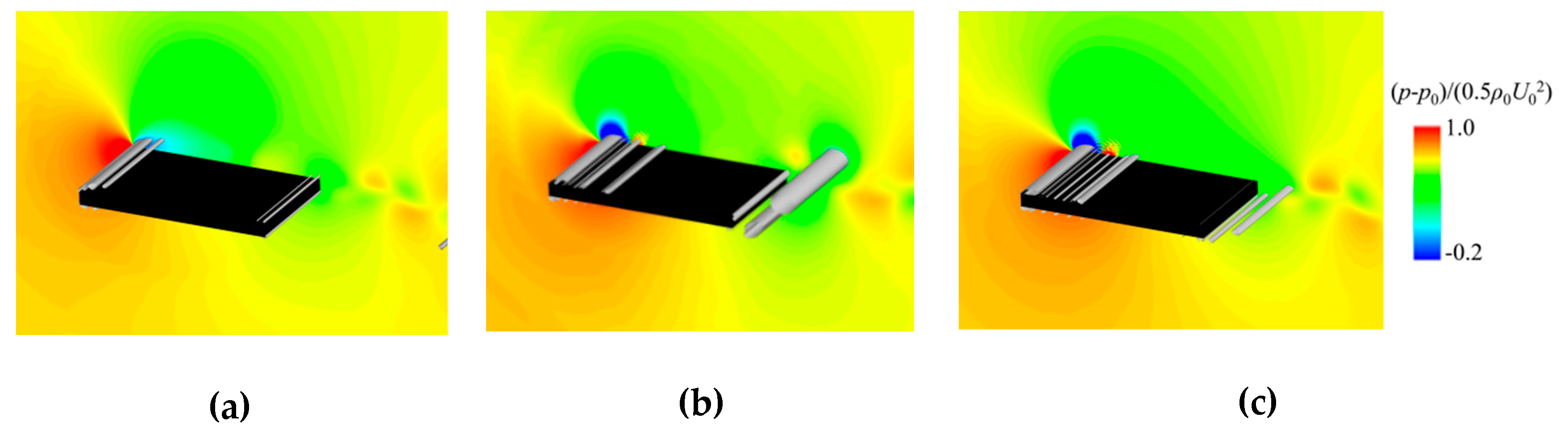
4.2. Lift Generation Mechanism by Control

The control effects for each installation surface of the actuators, as shown in Figure 14, are discussed in this section. Figure 14a,b give the time-averaged lift and time fluctuations of the lift coefficient, respectively. The actuators are driven with the time offset of t₀ = 0 and driving ratio of R = 50% for all the different installation surfaces. The results with these driving conditions for the control only on the top surface indicate the highest time-averaged lift coefficient in all the conditions of this research, as further discussed in Section 4.3.

As shown in Figure 14a, all the conditions of the installation surface show the increase of the time-averaged lift by the control. As seen in Figure 14b, for the control only on the bottom surface, the control effects on the lift fluctuations are smaller compared to those for other cases. This is because the flow is not largely separated on the bottom surface in the baseline flow, as shown in Figure 13b. As a result, the effect of the induced flow by the actuator, which is effective for suppression of flow separation, is relatively smaller. Meanwhile, the control only on the top surface produced the highest lift coefficient, where the time-averaged lift coefficient is increased by 11.6% compared to the baseline. The flow fields at the times for the large control effects around t/T = 0.2 and 0.35, as shown in Figure 14b, are discussed in the following paragraphs.

Figure 15 depicts the contours of the vorticity (left) and the vortices with the contours of the pressure (right) for the cases with and without control at the times for the local minimum of the fluctuating lift coefficient around t/T = 0.2 at each case (Figure 14b) and t/T = 0.35. As expressed in Figure 14b, the lift is sharply decreased at t/T = 0.18 and 0.22 for the control only on the top surface and both surfaces, respectively. This is because the separation vortices on the top surface are suppressed by the control on the top surface, as shown in Figure 15a and the pressure on the top surfaces is increased. Also, for the control on the top surface, the alleviation of this decrease, while maintaining the increase of the lift obtained in other time, leads to a much-improved time-averaged lift. This is a future problem to be solved.

As displayed in Figure 14b, the deeper decrease appears at the above-mentioned time of t/T = 0.22 in the control on both surfaces compared with the control only on the top surface. This is because the flow acceleration on the bottom surface occurs due to the induced flow by the actuator, as shown in Figure 16, where the velocity profile averaged during the up-stroke motion along the vertical position from the bottom surface, y_w, at the trailing edge. As a result, the velocity gradient on the bottom surface wall becomes steeper and hence a more intense vortex is shed from the trailing edge, as shown in Figure 15a. This decreases the pressure on the bottom surface and suppresses the lift coefficient so that the increase of the time-averaged lift coefficient for the control on both surfaces compared with the baseline case is limited, as shown in Figure 14a.

Figure 15b reveals that the vortex shed from the trailing edge on the bottom surface at t/T = 0.35 becomes weaker for the control on the top surface and both surfaces than that for the baseline flow (Figure 13), which increases lift. This suppression of the vortex shedding from the bottom surface possibly occurs because the flow in the wake of the plate becomes stable due to the suppression of the flow separation on the top surface by the control during the earlier time of t/T = 0.0–0.35. This implies that the lift enhancement by the suppression of the vortex shedding on the bottom surface, which is the mechanism similar to the feathering motion of insect flight [15,16], is realized by the plasma actuator. Particularly, the highest lift around t/T = 0.3–0.5 for the control only on the top surface, compared to the other conditions of the installation surface, contributes to the highest time-averaged lift, as shown in Figure 14a. In the following section, the effects of the driving conditions, such as the driving ratio and time offset for the control only on the top surface, are explored.

4.3. Effects of Driving Conditions

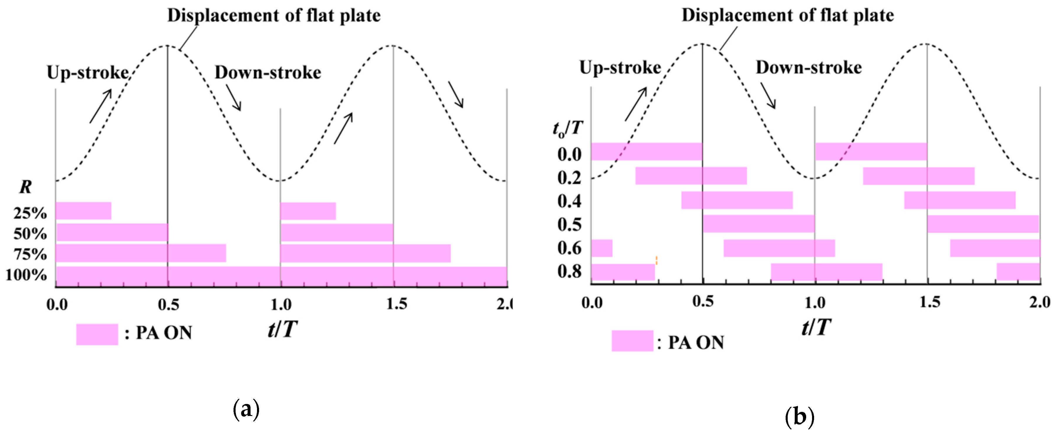
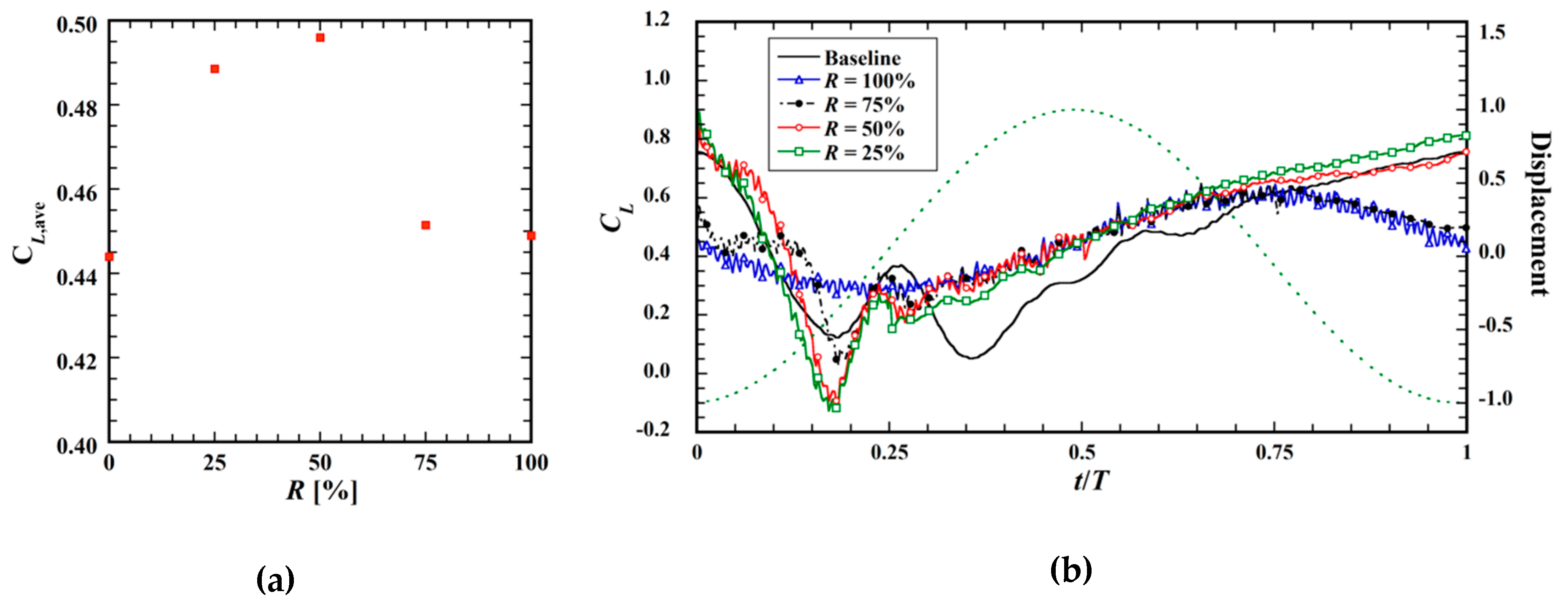
4.3.1. Effects of Driving Ratio

Figure 17 exhibits the effects of the driving ratio, R, on the lift coefficient for the time offset of t₀/T = 0 for the control only on the top surface. As mentioned above, the case of R = 50% produced the highest time-averaged lift force in all the present conditions. In addition, the increase of the lift for the condition of R = 25% is comparable to the condition of R = 50%, which was discussed in the previous section. In the case of 25%, the lift coefficient increased particularly in the duration of t/T = 0.3–0.5, when the actuator is not driven. Figure 18 shows the vortices and the contours of the pressure around the oscillating plate at t/T = 0.35 for R = 25, 75 and 100%. Figure 18a presents that the vortex shedding from the trailing edge on the bottom surface is suppressed along with the suppression of the flow separation on the top surface while the actuator is driven, from t/T = 0.0–0.25, for R = 25%. This mechanism for the increase in lift is similar to that for R = 50% as aforementioned (Section 4.2).

As shown in Figure 17b, the fluctuations of the lift coefficient become smoother, particularly in the time range of t/T = 0.0–0.5 by the control with R = 100%. This is because the vortex shedding from the trailing edge becomes weaker due to the suppression of the flow separation on the top surface throughout the oscillation period, as illustrated in Figure 18c. The increases in the time-averaged lift for R = 75, 100% are quite small, as exhibited in Figure 17a. This can be explained by the decrease of the lift between t/T = 0.75–1.0 in comparison with the baseline flow. As shown in Figure 18b,c, the separation vortex from the leading edge on the upper surface, which contributes to the lift generation in the baseline case, is also suppressed during the down-stroke motion (t/T = 0.75). This suggests that the control in the down-stroke motion negatively affects lift. Accordingly, the control with the driving ratio of R = 50% is more effective in increasing lift.

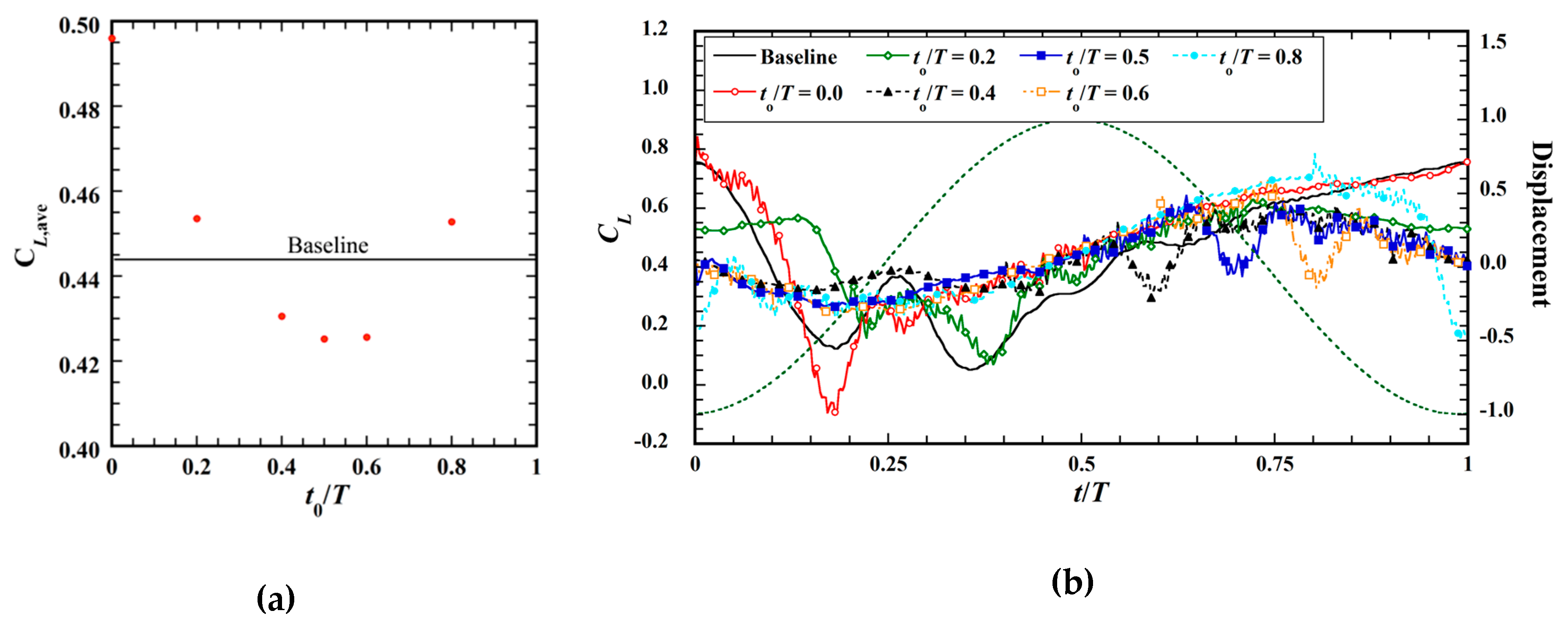
4.3.2. Effects of Time Offset

In this section, the effects of the time offset, t₀/T, on the lift for the control only on the top surface with R = 50% is discussed. Figure 19 depicts the lift coefficient for t₀/T = 0.0–0.8 for the baseline case. The time-averaged lift coefficient is increased under the conditions of t₀/T = 0.0, 0.2, 0.8 compared to baseline case, while lift is decreased under the conditions of t₀/T = 0.4, 0.5, 0.6. Especially, the conditions of t₀/T = 0.0 and 0.5 generated the highest and lowest coefficients, respectively. The lowest averaged lift around t₀/T = 0.5 is due to the suppression of the separation vortices on the top surface during the down-stroke motion, like the cases of R = 75, 100% with t₀/T = 0.0 mentioned above.

For the cases of t₀/T = 0.5 and 0.8, the local steep decreases of the lift in the up-stroke motion (t/T = 0.18, 0.35) in the baseline case disappears as displayed in Figure 19b. Figure 20 shows the vortices and the contours of the pressure for the time offset of t₀/T = 0.5. The vortex shedding from the trailing edge on the bottom surface observed in the baseline case at t/T = 0.18 is suppressed similarly to the case of R = 100%. This indicates that the suppression of the flow separation on the top surface in the down-stroke motion is also effective for the suppression of vortex shedding from the trailing edge in the following up-stroke motion; these findings illustrate a similar mechanism to that of the feathering motion produced by insects during flight [15,16]. However, by this control, the lift is significantly decreased in the down-stroke motion, precipitating the decrease of the time-averaged lift. To conclude this part of the research, the control during the up-stroke motion (t/T = 0.0–0.5) is effective for lift enhancement.

5. Conclusions

To investigate the control effects by the plasma actuator on the flow around an oscillating plate in a uniform flow, wind tunnel experiments and numerical simulations were performed. In the experiments, the flow with and without control was visualized. In addition, the lift fluctuations and flow fields around the plate were investigated with the numerical simulations based on the volume penalization method. The effects of the installation surface and driving conditions on lift enhancement were investigated.

In the baseline flow, the flow separation occurs from the leading edge on the top surface throughout most of the period. By continuously driving the plasma actuator installed near the leading edge on the top surface, the flow separation was almost suppressed while the flow was separated around the center of the plate in the up-stroke motion. These control effects were confirmed in both the experimental and predicted results.

In all the present control conditions of the installation surface, driving ratio and time offset, the driving of the actuator only on the top surface during the up-stroke motion shows most significantly enhances lift, whereas the time-averaged lift coefficient was increased by 11.6% compared to the baseline flow. This is because the vortex shedding from the bottom surface is suppressed in the up-stroke motion due to the stabilization of the wake, along with the suppression of the flow separation on the top surface by the control. In other words, it is possible for the plasma actuator to increase lift with a mechanism similar to the feathering motion of insect flight.

The control in the down-stroke motion successfully minimized decrease of lift in the up-stroke motion; however, this control also suppressed the flow separation of the vortices on the top surface in the down-stroke motion and the increase of the time-averaged lift was limited.

Although there is a possibility that increased lift could be achieved by more detailed adjustments to the driving conditions for the control by the actuators installed on both surfaces, the present results indicate that appropriate adjustment of the time for driving the actuator plays an important role in lift enhancement.

References

1. Liu, H.; Ravi, S.; Kolomenskiy, D.; Tanaka, H. Biomechanics and biomimetics in insect-inspired flight systems. Philos. Trans. R. Soc. B 2017, 371, 20150390. [Google Scholar] [CrossRef] [PubMed]
2. McMasters, J.H.; Henderson, M.L. Low-Speed Single-Element Airfoil Synthesis. 1979. Available online: https://ntrs.nasa.gov/archive/nasa/casi.ntrs.nasa.gov/19790015719.pdf (accessed on 22 February 2019).
3. Yousefi, K.; Razeghi, A. Determination of the critical Reynolds number for flow over symmetric NACA airfoils. In Proceedings of the AIAA Aerospace Sciences Meeting 2018, AIAA 2018, Kissimmee, FL, USA, 8–12 January 2018. [Google Scholar]
4. Mueller, T.J. Fixed and Flapping Wing Aerodynamics for Micro Air Vehicle Applications, Progress in Astronautics and Aeronautics; American Institute of Aeronautics and Astronautics: Reston, VA, USA, 2010; Volume 195. [Google Scholar]
5. Shyy, W.; Liang, Y.; Tang, J.; Viieru, D.; Liu, H. Aerodynamics of Low Reynolds Number Flyers; Cambridge University Press: New York, NY, USA, 2007. [Google Scholar]
6. Liu, H. Micro air vehicles. In Encyclopedia of Aerospace Engineering; Blockrey, R., Shyy, W., Eds.; John Wiley & Sons: Chichester, UK, 2010; ISBN 978-0-470-75440-5. [Google Scholar]
7. Floreano, D.; Wood, R.J. Science, technology and the future of small autonomous drones. Nature 2015, 521, 460–466. [Google Scholar] [CrossRef] [PubMed] [Green Version]
8. Percin, M.; van Oudheusden, B.W.; Eisma, H.E.; Remes, B.D.W. Three-dimensional vortex wake structure of a flapping-wing micro aerial vehicle in forward flight configuration. Exp. Fluids 2014, 55, 1806. [Google Scholar] [CrossRef]
9. Nakatani, Y.; Suzuki, K.; Inamuro, T. Flight control simulations of a butterfly-like flapping wing-body model by the immersed boundary-lattice Boltzmann method. Comput. Fluids 2016, 133, 103–115. [Google Scholar] [CrossRef]
10. Phan, H.V.; Nguyen, Q.V.; Truong, Q.T.; Truong, T.V.; Park, H.C.; Goo, N.S.; Byun, D.; Kim, M.J. Stable vertical takeoff of an insect-mimicking flapping-wing system without guide implementing inherent pitching stability. J. Bionic Eng. 2012, 9, 391–401. [Google Scholar] [CrossRef] [Green Version]
11. Jang, J.H.; Yang, G.-H. Design of wing root rotation mechanism for dragonfly-inspired micro air vehicle. Appl. Sci. 2018, 8, 1868. [Google Scholar] [CrossRef]
12. Sivasankaran, P.N.; Ward, T.A.; Salami, E.; Viyapuri, R.; Fearday, C.J.; Johan, M.R. An experimental study of elastic properties of dragonfly-like flapping wings for use in biomimeticmicro air vehicles (BMAVs). CSAA Chin. J. Aeronaut. 2017, 30, 726–737. [Google Scholar] [CrossRef]
13. Azuma, A.; Azuma, S.; Watanabe, I.; Furuta, T. Flight mechanics of a dragonfly. J. Exp. Biol. 1985, 116, 79–107. [Google Scholar]
14. Thomas, A.L.; Taylor, G.K.; Srygley, R.B.; Nudds, R.L.; Bomphrey, R.J. Dragonfly flight: Free-flight and tethered flow visualizations reveal a diverse array of unsteady lift-generating mechanisms, controlled primarily via angle of attack. J. Exp. Biol. 2004, 207, 4299–4323. [Google Scholar] [CrossRef]
15. Dickinson, M.H.; Lehmann, F.-O.; Sane, S.P. Wing rotation and the aerodynamic basis of insect flight. Science 1999, 284, 1954–1960. [Google Scholar] [CrossRef] [PubMed]
16. Iida, A.; Nakamura, M.; Jida, S.; Fukawa, M.; Ogisu, H.; Mizuno, A. Correlation analysis in terms of unsteady aerodynamic force and flow field around a flying insect. Trans. JSME B 2007, 73, 1781–1789. (In Japanese) [Google Scholar] [CrossRef]
17. Yousefi, K.; Saleh, R. Three-dimensional suction flow control and suction jet length optimization of NACA 0012 wing. Meccanica 2015, 50, 1481–1494. [Google Scholar] [CrossRef] [Green Version]
18. Zhang, Z.Y.; Zhang, W.L.; Chen, Z.; Sun, X.H.; Xia, C.C. Suction control of flow separation of a low-aspect-ratio wing at low Reynolds-number. Fluid Dyn. Res. 2018, 50. [Google Scholar] [CrossRef]
19. Yousefi, K.; Saleh, R.; Zahedi, P. Numerical study of blowing and suction slot geometry optimization on NACA 0012 airfoil. J. Mech. Sci. Technol. 2014, 28, 1297–1310. [Google Scholar] [CrossRef] [Green Version]
20. Yousefi, K.; Saleh, R. The effects of trailing edge blowing on aerodynamic characteristics of the NACA 0012 airfoil and optimization of the blowing slot geometry. J. Theor. Appl. Mech. 2014, 52, 165–179. [Google Scholar]
21. You, D.; Moin, P. Active control of flow separation over an airfoil using synthetic jets. J. Fluid. Struct. 2008, 24, 1349–1357. [Google Scholar] [CrossRef]
22. Traub, L.W.; Miller, A.; Rediniotis, O. Effects of synthetic jet actuation on a ramping NACA 0015 airfoil. J. Aircr. 2004, 41, 1153–1162. [Google Scholar] [CrossRef]
23. Velasco, D.; Mejia, O.L.; Laín, S. Numerical simulations of active flow control with synthetic jets in a Darrieus turbine. Renew. Energ. 2017, 113, 129–140. [Google Scholar] [CrossRef]
24. Miyamoto, T.; Yokoyama, H.; Iida, A. Suppression of aerodynamic tonal noise from an automobile bonnet using a plasma actuator. SAE Int. J. Passeng. Cars Mech. Syst. 2017, 10, 712–720. [Google Scholar] [CrossRef]
25. Singhal, A.; Castañeda, D.; Webb, N.; Samimy, M. Control of dynamic stall over a NACA0015 airfoil using plasma actuators. AIAA J. 2017, 56, 78–89. [Google Scholar] [CrossRef]
26. Inasawa, A.; Ninomiya, C.; Asai, M. Suppression of total trailing-edge noise from an airfoil using a plasma actuator. AIAA J. 2013, 51, 1695–1702. [Google Scholar] [CrossRef]
27. Post, M.L.; Corke, T.C. Separation control using plasma actuators: Dynamic stall vortex control on oscillating airfoil. AIAA J. 2006, 44, 3125–3135. [Google Scholar] [CrossRef]
28. Roth, J.R.; Dai, X. Optimization of the aerodynamic plasma actuator as an electrohydrodynamic (EHD) electrical device. In Proceedings of the 44th AIAA Aerospace Sciences Meeting and Exhibit, Reno, NV, USA, 9–12 January 2006. AIAA-2006-1203. [Google Scholar]
29. Esfahani, A.; Webb, N.; Samimy, M. Stall cell formation over a post-stall airfoil: Effects of active perturbations using plasma actuators. Exp. Fluids 2018, 59. [Google Scholar] [CrossRef]
30. Yokoyama, H.; Tanimoto, I.; Iida, A. Experimental tests and aeroacoustic simulations of the control of cavity tone by plasma actuators. Appl. Sci. 2017, 7, 790. [Google Scholar] [CrossRef]
31. Kusumoto, M.; Yokoyama, H.; Angland, D.; Iida, A. Control of aerodynamic noise from cascade of flat plates by plasma actuators. Trans. JSME 2017, 83, 1–16. (In Japanese) [Google Scholar] [CrossRef]
32. Lele, S.K. Compact finite difference schemes with spectral-like resolution. J. Comput. Phys. 1992, 103, 16–42. [Google Scholar] [CrossRef]
33. Angot, P.; Bruneau, C.-H.; Frabrie, P. A penalization method to take into account obstacles in viscous flows. Numer. Math. 1999, 81, 497–520. [Google Scholar] [CrossRef]
34. Liu, Q.; Vasilyev, O.V. A Brinkman penalization method for compressible flows in complex geometries. J. Comput. Phys. 2007, 227, 946–966. [Google Scholar] [CrossRef]
35. Tanaka, Y.; Yokoyama, H.; Iida, A. Forced-oscillation control of sound radiated from the flow around a cascade of flat plates. J. Sound Vib. 2018, 431, 248–264. [Google Scholar] [CrossRef]
36. Suzen, Y.B.; Hung, P.G.; Jacob, J.D.; Ashpis, D.E. Numerical simulations of plasma based flow control applications. In Proceedings of the 35th Fluid Dynamics Conference and Exhibit, Toronto, ON, Canada, 6–9 June 2005. AIAA-paper, No. AIAA-2005–4633. [Google Scholar]
37. Kaneda, I.; Sekimoto, S.; Nonomura, T.; Asada, K.; Oyama, A.; Fujii, K. An effective three-dimensional layout of actuation body force foe separation control. Int. J. Aerosp. Eng. 2012, 2012, 786960. [Google Scholar] [CrossRef]
38. Forte, M.; Jolibois, J.; Pons, J.; Moreau, E.; Touchard, G.; Cazalens, M. Optimization of a dielectric barrier discharge actuator by stationary and non-stationary measurements of the induced flow velocity: Application to airflow control. Exp. Fluids 2007, 43, 917–928. [Google Scholar] [CrossRef]
Figure 1. A dielectric-barrier-discharge plasma actuator. (a) Schematic sketch; (b) Picture of the present actuator.
Applsci 09 00776 g001
Figure 2. Schematic of the oscillating plate.
Applsci 09 00776 g002
Figure 3. Cross-section of plasma actuator.
Applsci 09 00776 g003
Figure 4. The driving conditions of plasma actuators for two periods (2T), where T is an oscillating period and t = 0 represents the time for the bottom dead center of the oscillating motion. (a) Conditions with varied driving ratio (t0/T = 0.0); (b) Conditions with varied time offset (R = 50%).
Applsci 09 00776 g004
Figure 5. The experimental setup with link mechanism for oscillation of the plate. (a) Photograph; (b) Schematic sketch.
Applsci 09 00776 g005
Figure 6. Visualized flow field in experiment and predicted streamline for a fixed plate with α = 4°.
Applsci 09 00776 g006
Figure 7. Predicted contours of the amplitude and vectors of the body force by plasma actuator, where the actuator is installed on top surface of the plate.
Applsci 09 00776 g007
Figure 8. Computational grid and domain of flow around an oscillating plate. (a) Computational grid; (b) Computational domain and boundary conditions.
Applsci 09 00776 g008
Figure 9. Predicted variation of lift coefficient for the control condition of t0/T = 0.0 and R = 50% with the original and finer grids.
Applsci 09 00776 g009
Figure 10. The visualized flow pattern and predicted streamlines (upper right in each figure) around the oscillating plate with and without control by the actuator on the top surface (R = 100%), where T is an oscillation period and t = 0 represents the time for the bottom dead center of the oscillating motion.
Applsci 09 00776 g010
Figure 11. Measured and predicted profiles of mean streamwise velocity Uh at the downstream position from the leading edge with the distance of 4.5b from the leading edge are shown in the left figure, where y/b = 0.5 is corresponding to position of plate wall. The right figure shows the profiles of turbulent intensity. These figures show both the predicted profiles agree with those measured for the cases with and without control by the plasma actuator [31].
Applsci 09 00776 g011
Figure 12. The time fluctuations of lift coefficient in the baseline flow. The dashed line represents the displacement of oscillating plate without the dimension of amplitude.
Applsci 09 00776 g012
Figure 13. The flow field around the oscillating plate in the baseline flow. (a) The iso-surfaces of second invariant (q/(U0/b)2 = 0.1) of velocity gradient tensor and contours of pressure coefficient (p-p0)/(0.5ρ0U02), where p0 is the ambient pressure; (b) The contours of vorticity.
Applsci 09 00776 g013
Figure 14. The lift coefficient for the baseline and controlled cases for each installation surface. (a) The time-averaged lift coefficient; (b) The time fluctuations of lift coefficient during the time period of the oscillation, where the dashed line represents the displacement of oscillating plate without the dimension of amplitude.
Applsci 09 00776 g014
Figure 15. Flow fields for the baseline case and the case for the control by the actuator installed on the top surface. The left figures show the iso-surfaces of second invariant (q/(U0/b)2 = 0.1) of velocity gradient tensor with the contours of pressure coefficient (p-p0)/(0.5ρ0U02). The right figures show the contour of vorticity. (a) Time corresponding to local minimum force coefficient; (b) The time of t/T = 0.35.
Applsci 09 00776 g015
Figure 16. Time-averaged velocity profile at the trailing edge along the vertical position from the bottom surface, yw, during the up-stroke motion.
Applsci 09 00776 g016
Figure 17. Effects of the driving ratio on the lift coefficient (t0/T = 0) for the control only on the top surface. (a) Time-averaged lift coefficient; (b) Time fluctuations of lift coefficient.
Applsci 09 00776 g017
Figure 18. Iso-surfaces of second invariant (q/(U0/b)2 = 0.1) of velocity gradient tensor and contours of pressure coefficient (p-p0)/(0.5ρ0U02) around the oscillating plate for the control only on the top surface (t0/T = 0.0), where p0 is the ambient pressure. (a) Driving ratio of R = 25%; (b) R = 75%; (c) R = 100%.
Applsci 09 00776 g018
Figure 19. Lift with each time offset for the control only on the top surface (R = 50%). (a) Time-averaged lift coefficient; (b) Time fluctuations of lift coefficient.
Applsci 09 00776 g019
Figure 20. Iso-surfaces of second invariant of velocity gradient tensor and contours of pressure coefficient around oscillating plate under the condition of t0/T = 0.5. (a) t/T = 0.18; (b) t/T = 0.75; (c) t/T = 0.94.
Applsci 09 00776 g020