A Low-Order Series Approximation of Thin-Bed PP-Wave Reflections

Abstract

The study of thin-bed seismic phenomena is important in crustal, exploration and engineering seismology. Presently, seismic reflectivity theories based on single-interface assumption are widely used though they are only suitable for thick deposits. Thin-bed reflectivity theories are established on complex propagator matrices and are difficult to be applied to reveal thin-bed properties directly. Therefore, an approximation of thin-bed PP-wave reflection coefficients (R_PP) is derived in this paper. First, the relationship between thin-bed R_PP and incidence angles is analyzed through series expansion method. For PP-wave, its reflection coefficients are even power series functions of sine incidence angles. Then, for small incidence, R_PP of the thin bed is further simplified into a second-order series approximation with respect to the sine incidence angles. Simulations and accuracy analyses of the approximate formula show that approximation errors are smaller than 5% as the incidence angles smaller than 20 degrees. Based on this approximate formula, an approach is given for estimating thin-bed properties including P-wave impedance ratios and thickness. The estimation approach is applied in properties estimation of a thin bed model. Perfect performances of the model example show the future potentiality of the approximate formula in thin-bed Amplitude-Versus-Offset (AVO) analysis and inversion.

1. Introduction

Seismic wave propagation in thin-bed models has been a hot topic of interest to crustal, exploration and engineering seismologists for many years [1,2,3]. In geodynamics study, stable deposited basins of the upper crust are thin-bed models under low-frequency seismic detection [1]. In fossil energy exploration, large or relatively simple structural reservoirs have been widely explored and become depleted and exhausted at present [4]. Locating and detecting the existence of stratigraphic lithologic reservoirs are gaining more and more attention. For some sedimentary basins, such as Williston Basin in America [5,6,7], Alberta Basin in Canada [8,9], SongLiao and Tarim Basins in China [10,11], lithologic reservoirs are composed of thin beds with the thicknesses below the vertical resolution limits [12]. Meanwhile, thin-bed problems are also faced in engineering exploration, such as monitoring CO₂ storage at Sleipner in the Norwegian North Sea [2,13,14,15]. Therefore, seismic responses of a thin bed, which carry information of stratigraphic structure, lithology and pore fluid, are significantly important to crustal, exploration and engineering research.

Differed significantly from single-interface cases, seismic responses of a thin bed are composed of reflections from the top and bottom interfaces, including the interbed multiples and converted reflections [16,17]. Therefore, current AVO analysis techniques based on the Zoeppritz equations and their corresponding approximations for a single interface are generally inefficient for the thin-bed reflections [18]. The reflectivity theory and seismic characteristics of thin-bed models have been discussed for several decades [12,19,20,21,22,23,24,25].

Normal seismic responses of a thin bed are widely discussed and mainly focused on the relationship of reflected amplitude and thin-bed thickness [12,24,25,26,27]. For arbitrary incidence, Liu and Schmitt derived an analytical approximation of a thin bed in acoustic media without considering the interbed multiples [20]. Rubino and Velis extended thin-bed AVO analysis from acoustic media to elastic media based on Liu and Schmitt’s work [21]. Yang et al. gave approximate formulas of thin-bed reflections in elastic media under the assumptions of small incidence angles and weak impedance contrasts [22]. These approximations show as relatively compact forms, but all ignore the contributions of interbed multiples and converted waves. Juhlin and Young ever pointed out when the contrast of elastic properties between the thin layer and its surrounding rock increases, it is necessary to consider the contributions of the interbed multiples and converted waves [17].

The contributions of interbed waves on thin-bed reflections have been considered by many researchers. Thomson [28] and Haskell [29] proposed a matrix method that transfers displacements and stresses through successive layers in multi-layered media. Brekhovskikh established the propagator matrices of displacements and stresses in multi-layered media as the seismic waves defined by displacement potential functions [19]. Restrepo et al. presented a closed-form Green’s function in the frequency wavenumber domain for a layered, elastic half-space model for SH wave propagation [30]. Yang et al. derived displacement reflection/transmission (R/T) coefficient equations of a thin bed and simplified them into pseudo-Zoeppritz equations under thin-bed assumption [23]. Kumar et al. presented reflection coefficients due to incident plane SH-wave at an anisotropic magnetoelastic layer sandwiched between two inhomogeneous viscoelastic half-spaces [31]. Sahu et al. gave reflection and transmission of plane waves through isotropic medium sandwiched between two highly anisotropic half-spaces [32]. Paswan et al. studied the reflection and transmission of a plane wave through a fluid layer of finite width sandwiched between two dissimilar monoclinic elastic half-spaces [33]. Singh et al. gave reflection and transmission matrix equations of P-wave at the interfaces of the layered sandwiched model comprised of a water layer between an upper ice half-space and a lower isotropic elastic half-space [34]. These matrix formulas considered all wave modes including interbed multiple waves and converted waves. However, to a certain extent, the complex forms of matrix equations limited their application in thin-bed AVO analysis and inversion. Therefore, thin-bed reflected approximate formulas, which consider the effects of all wave modes and have relatively compact forms simultaneously, are needed for thin-bed AVO analysis and inversion.

In this paper, we first propose a series approximation of thin-bed R_PP under the small-incidence assumption, and test accuracy of the approximate formula with four representative thin-bed models through numerical analysis. And then we give an approach to estimate the thin-bed properties with this approximation.

2. R/T Coefficients Expressed by Series Functions

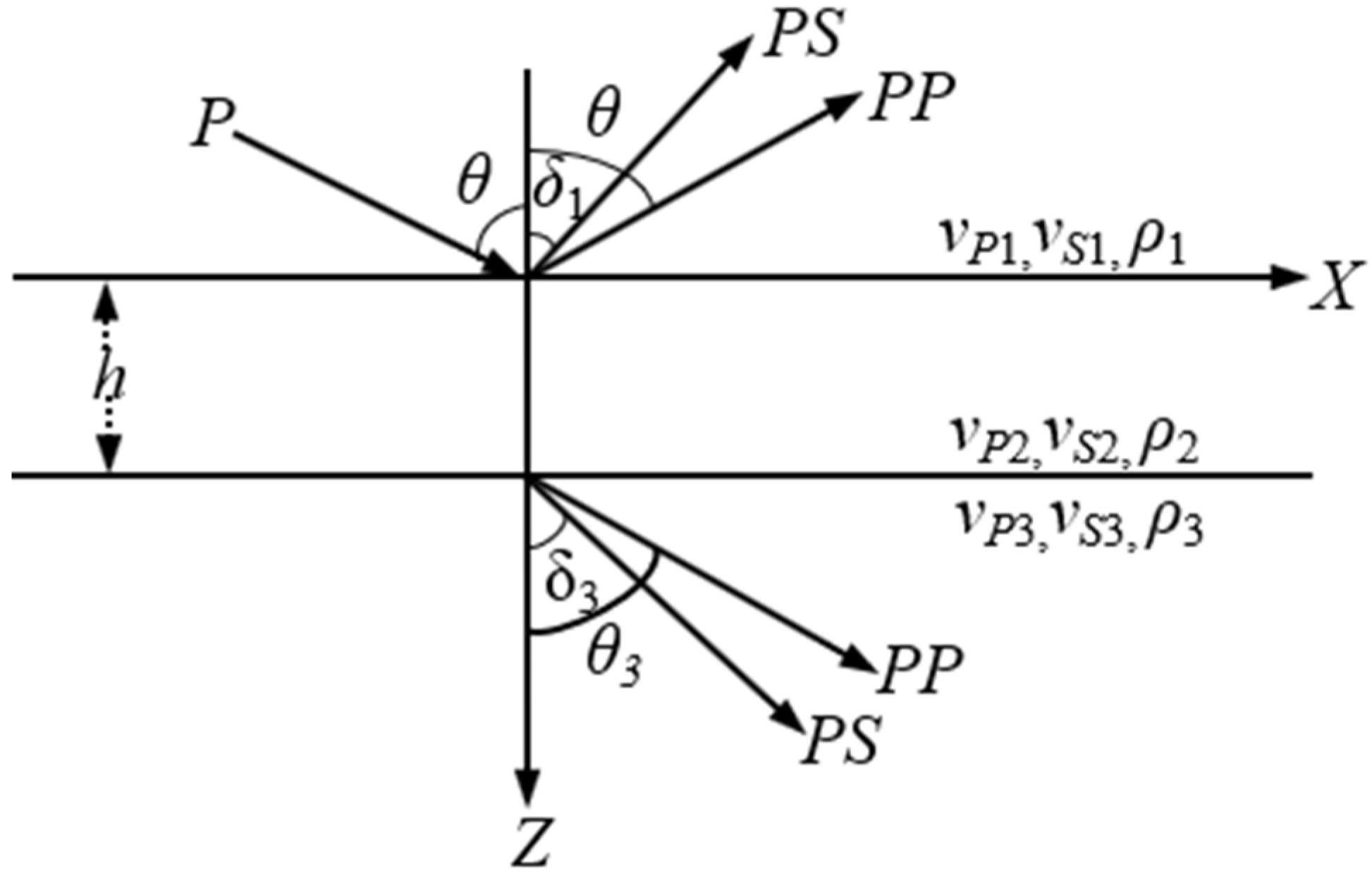
For a thin bed in elastic isotropic media, as shown in Figure 1, the exact displacement R/T coefficient equations for the P-wave incident are as follows [23],

$$M{\left[\begin{array}{cccc}{R}_{PP}& R_{PS}& T_{PP}& T_{PS}\end{array}\right]}^T=n$$

(1)

where R_PP, R_PS, T_PP, T_PS are displacement R/T coefficients of P-waves and converted S-waves, respectively; M is a 4 × 4 matrix, n is a 4 × 1 vector, which is presented in Appendix A in detail.

According to Cramer’s rule, the displacement R/T coefficients R_PP, R_PS, T_PP, T_PS can be calculated. When the thin-bed thickness is equal to zero, Equation (1) will be reduced to that for R/T coefficients equations of a single interface between the thin-bed roof and floor, which is consistent with the Zoeppritz equations [35].

From Equation (1), seismic theoretical characteristics analysis of a thin bed is easily achieved. However, complicated matrix calculations prevent its application in thin-bed AVO analysis and inversion. To solve Equation (1) approximately, the trigonometric function parameters are rewritten as a series expansion of sine incidence angle (see Appendix B).

Substituting Equations (A18)–(A34) into Equation (1), the elements of M and n are all expressed by series functions of sine incidence angle (sinθ). If the elements are even or odd series functions of sinθ, we mark them by ‘even’ or ‘odd’ in Equation (1) respectively as follows,

$$\left[\begin{array}{cccc}odd& even& odd& even\\ even& odd& even& odd\\ even& odd& even& odd\\ odd& even& odd& even\end{array}\right]\left[\begin{array}{c}{R}_{PP}\\ R_{PS}\\ T_{PP}\\ T_{PS}\end{array}\right]=\left[\begin{array}{c}odd\\ even\\ even\\ odd\end{array}\right]$$

(2)

From Equation (2), it can be seen that R_PP, T_PP are even power series functions of sinθ, while R_PS, T_PS are odd power series functions of sinθ. Therefore, R_PP, R_PS, T_PP, T_PS can be expressed by series functions of sinθ as follows,

$$\{\begin{array}{l}{R}_{PP}={\displaystyle \sum _{n=0}^{\infty }{A}_{2n}{\sin }^{2n}\theta }\\ R_{PS}={\displaystyle \sum _{n=0}^{\infty }{A}_{2n+1}{\sin }^{2n+1}\theta }\\ T_{PP}={\displaystyle \sum _{n=0}^{\infty }{B}_{2n}{\sin }^{2n}\theta }\\ T_{PS}={\displaystyle \sum _{n=0}^{\infty }{B}_{2n+1}{\sin }^{2n+1}\theta }\end{array}$$

(3)

where A and B are coefficients of series functions.

3. Approximate Formula of PP-Wave Reflections

For small incidence, sinⁿθ decreases rapidly with increasing n in Equation (3). R_PP can be simplified into a second-order series approximation of sine incidence angle via a series truncation procedure as follows,

$$R_{PP}\approx A_0+A_2{\sin }^2\theta$$

(4)

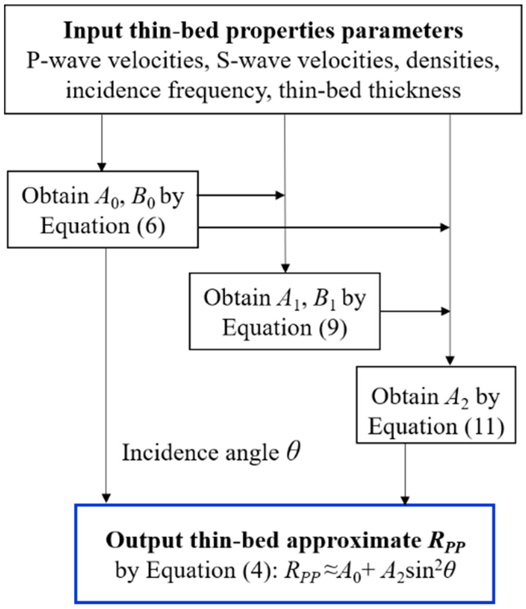
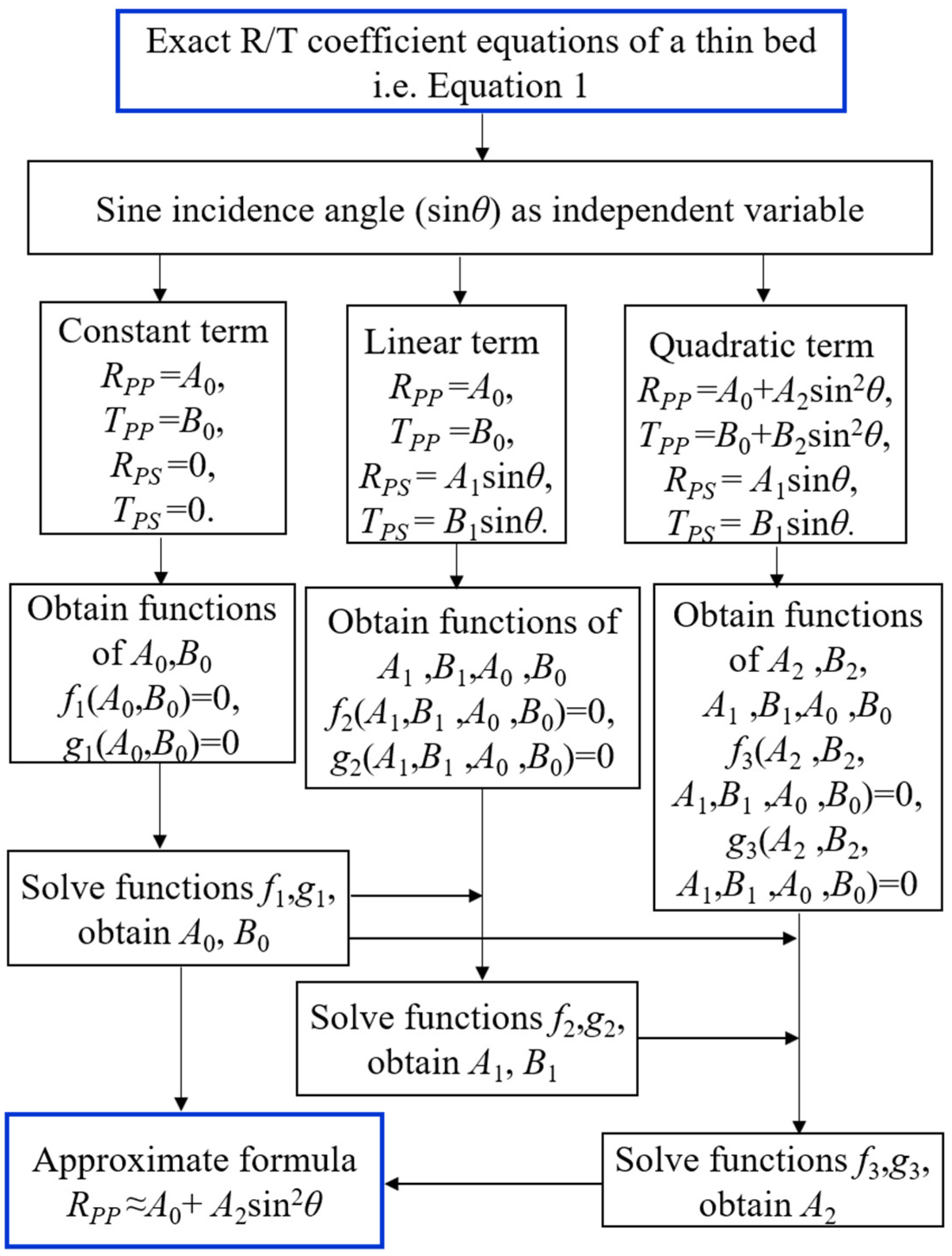
Figure 2 shows the simplified procedure of the approximate formula from the exact R/T coefficient equation, i.e., Equation (1), in detail. Taking sinθ as an independent variable, we can obtain A₀, B₀, A₁, B₁, A₂ in turn from the constant term, linear term and quadratic term of sinθ in Equation (1), respectively.

Considering the constant term of sine incidence angle in Equation (1), i.e., normal incidence, then R_PP = A₀, T_PP = B₀, R_PS = 0, T_PS = 0. Equation (1) is simplified as

$$\{\begin{array}{l}\left(\cos \tau +j\frac{z_{P1}}{z_{P2}}\sin \tau \right)A_0+B_0=\cos \tau -j\frac{z_{P1}}{z_{P2}}\sin \tau \\ \left(\cos \tau +j\frac{z_{P2}}{z_{P1}}\sin \tau \right)A_0-\frac{z_{P3}}{z_{P1}}{B}_0=j\frac{z_{P2}}{z_{P1}}\sin \tau -\cos \tau \end{array}$$

(5)

where τ = ωh/v_P2, z_P = ρv_P are P-wave impedances and their subscripts 1,2,3 indicate three layers of the single thin bed, respectively; j is an imaginary symbol.

Solving Equation (5), there are

$$A_0=\left[\left(\frac{z_{P3}}{z_{P1}}-1\right)\cos \tau +j\left(\frac{z_{P2}}{z_{P1}}-\frac{z_{P3}}{z_{P2}}\right)\sin \tau \right]/m_0$$

(6a)

$$B_0=2/m_0$$

(6b)

with m₀ = (z_P3/z_P1 + 1)cosτ + j(z_P2/z_P1 + z_P3/z_P2)sinτ.

When the thickness is equal to zero, the thin-bed model becomes a single interface constituted by the roof and floor of the original thin bed. Equation (6) is simplified as

$$A_0=\frac{z_{P3}-z_{P1}}{z_{P3}+z_{P1}}$$

(7a)

$$B_0=\frac{2z_{P1}}{z_{P3}+z_{P1}}$$

(7b)

which are consistent with the normal reflection and transmission coefficients given by Zoeppritz [35], respectively.

Considering the linear term of sine incidence angle in Equation (1), then R_PP = A₀, T_PP = B₀, R_PS = A₁sinθ, T_PS = B₁sinθ. Equation (1) is simplified as

$$\{\begin{array}{cc}\hfill a_1{A}_1-B_1& =\left(\frac{a_3}{d_1}-\cos q\right)(1+A_0)+l_1{l}_2{B}_0\hfill \\ & +j\left(l_1\sin \tau +\frac{2}{r_1}\frac{z_{S1}}{z_{S2}}\sin q-\frac{2l_1}{r_2}\sin q\right)(1-A_0)\hfill \\ \hfill a_2{A}_1+\frac{z_{S3}}{z_{S1}}{B}_1& =j\left(a_5-\frac{z_{S2}}{z_{S1}}\sin q\right)(1+A_0)\hfill \\ & +\left(\frac{2}{r_1}\cos q-\frac{2a_3{l}_1}{r_2}\frac{z_{S2}}{z_{S1}}\right)(1-A_0)-a_4{B}_0\hfill \end{array}$$

(8)

where q = ωh/v_S2, d₁ = ρ₂/ρ₁; z_S = ρv_S are S-wave impedances, r = v_P/v_S are the ratios of P-wave velocities to S-wave velocities, their subscripts 1, 2, 3 refer to three layers of the single thin bed respectively. l_k = v_Pk + 1/v_Pk are the ratios of the P-wave velocities in adjacent layers with k = 1, 2, a₁~a₅ are presented in Appendix C.

Solving Equation (8), there are

$$\begin{array}{l}{A}_1=\frac{1}{m_1}\left[\left(\frac{a_3}{d_1}-\cos q\right)\frac{z_{S3}}{z_{S1}}+j\left(a_5-\frac{z_{S2}}{z_{S1}}\sin q\right)\right](1+A_0)+\frac{1}{m_1}\left(l_1{l}_2\frac{z_{S3}}{z_{S1}}-a_4\right)B_0\\ +\frac{1}{m_1}\left[\left(\frac{1}{r_1}-\frac{l_1}{r_2}\frac{z_{S2}}{z_{S1}}\right)a_6+\frac{2l_1}{r_2}\cos \tau \frac{z_{S2}}{z_{S1}}+j{l}_1\sin \tau \frac{z_{S3}}{z_{S1}}\right](1-A_0)\end{array}$$

(9a)

and

$$\begin{array}{l}{B}_1=\frac{1}{m_1}\left(1-\frac{a_2{a}_3}{d_1}+j{a}_1{a}_5\right)(1+A_0)-\frac{1}{m_1}\left[l_1{l}_2{a}_2+\left(\cos q+j\sin q\right)a_4\right]B_0\\ +\frac{1}{m_1}\left[\frac{2}{r_1}-j{a}_2{l}_1\sin \tau +\frac{2l_1}{r_2}\frac{z_{S2}}{z_{S1}}\left(a_1\cos \tau -1\right)\right](1-A_0)\end{array}$$

(9b)

with m₁ = (z_S3/z_S1 + 1)cosq + j(z_S2/z_S1 + z_S3/z_S2)sinq. a₆ is given in Appendix C.

Considering the quadratic term of sine incidence angle in Equation (1), then R_PP = A₀ + A₂sin²θ, T_PP = B₀ + B₂sin²θ, R_PS = A₁sinθ, T_PS = B₁sinθ. Equation (1) is simplified as

$$\begin{array}{l}\left(\cos \tau +j\frac{z_{P1}}{z_{P2}}\sin \tau \right)A_2+B_2=\left(b_1+j{b}_3\frac{z_{P1}}{z_{P2}}\right)\left(1+A_0\right)\\ +b_6\left(1-A_0\right)+\frac{l_1^2{l}_2^2}{2}{B}_0+\frac{l_1{l}_2}{r_3}{B}_1\\ +\left(b_1+\frac{1}{r_1}\cos \tau +\frac{a_3}{r_1{d}_1}+j\frac{2\sin \tau }{r_1^2}\frac{z_{P1}}{z_{P2}}\right)A_1\end{array}$$

(10a)

and

$$\begin{array}{l}\left(\cos \tau +j\frac{z_{P1}}{z_{P2}}\sin \tau \right)A_2+B_2=\left(b_1+j{b}_3\frac{z_{P1}}{z_{P2}}\right)\left(1+A_0\right)\\ +b_6\left(1-A_0\right)+\frac{l_1^2{l}_2^2}{2}{B}_0+\frac{l_1{l}_2}{r_3}{B}_1\\ +\left(b_1+\frac{1}{r_1}\cos \tau +\frac{a_3}{r_1{d}_1}+j\frac{2\sin \tau }{r_1^2}\frac{z_{P1}}{z_{P2}}\right)A_1\end{array}$$

(10b)

with b₁~b₆ are presented in Appendix C.

Solving Equation (10), there is

$$\begin{array}{l}{A}_2=\frac{1}{m_0}\left[-\frac{l_1^2}{2}\tau \sin \tau +2\frac{a_3{l}_1^2}{r_2^2}\left(d_1-1\right)+\frac{2}{r_1^2}\cos \tau +b_1\frac{z_{P3}}{z_{P1}}+j{b}_3\frac{z_{P3}}{z_{P2}}\right]\left(1+A_0\right)\\ +\frac{1}{m_0}\left(b_6\frac{z_{P3}}{z_{P1}}+\frac{2j{b}_2{l}_1}{r_1^2}+j{b}_4\frac{z_{P2}}{z_{P1}}\right)\left(1-A_0\right)+\frac{b_5}{m_0}\left[l_1{l}_2\left(\frac{r_3^2}{4}-1\right)B_0+\left(\frac{r_3}{2}-1\right)B_1\right]\\ +\frac{1}{m_0}\left[\begin{array}{l}\left(b_1+\frac{\cos \tau }{r_1}\right)\frac{z_{P3}}{z_{P1}}+\frac{2}{r_1^2}\cos \tau +l_1{a}_3\left(\frac{2}{r_2^2}\frac{z_{P2}}{z_{P1}}+\frac{1}{r_1}\frac{z_{P3}}{z_{P2}}\right)\\ +\frac{2j\sin \tau }{r_1^2}\frac{z_{P3}}{z_{P2}}+j\frac{\sin \tau }{r_1}\frac{z_{P2}}{z_{P1}}-j\frac{b_2{l}_1}{r_1}\end{array}\right]A_1\end{array}$$

(11)

Equations (4) with (6a) and (11) constitute the wholly second-order series approximation of thin-bed R_PP, algorithmic steps of which are shown in Figure 3 detailly. The intercept and gradient of the approximate formula are dependent on frequency, which is greatly different from those of a single interface [36]. It is worthy to notice that, the approximate formula can be further simplified for ultra-thin bed cases by introducing in the approximations of sinτ ≈ τ, sinq ≈ q, cosτ ≈ 1, and cosq ≈ 1.

4. Accuracy Analysis

We tested the accuracy of the second-order series approximation on four representative thin-bed models, including (1) high-impedance thin bed, (2) low-impedance thin bed, (3) low-to-high impedance transition thin bed, and (4) high-to-low impedance transition thin bed.

Table 1. Rock properties of thin-bed models, units of velocities and densities are m/s and g/cm³, respectively.

	Layer No.	vP	vS	ρ	R1	R2
Model 1	1	3000	1414	2.29	/	/
	2	3800	2103	2.43	0.1468	–0.1468
	3	3000	1414	2.29	/	/
Model 2	1	3000	1414	2.29	/	/
	2	2400	897	2.17	−0.1376	0.1376
	3	3000	1414	2.29	/	/
Model 3	1	3000	1414	2.29	/	/
	2	3200	1586	2.33	0.0409	0.0388
	3	3400	1759	2.37	/	/
Model 4	1	3400	1759	2.37	/	/
	2	3200	1586	2.33	−0.0388	–0.0409
	3	3000	1414	2.29	/	/

lists rock properties of these models, including P-wave velocity (v_P), S-wave velocity (v_S), density (ρ), the normal-incident P-wave reflection coefficient of thin-bed top-interface (R₁), as well as the normal-incident P-wave reflection coefficient of thin-bed bottom-interface (R₂).

We compare the second-order series approximation and the true value of thin-bed R_PP in Figure 4, Figure 5, Figure 6 and Figure 7 for Models 1–4 respectively. For a better understanding of differences between thin-bed and single-interface responses, R_PP of thin-bed top- and bottom- interfaces based on the Zoeppritz equations are also curved in Figure 4, Figure 5, Figure 6 and Figure 7. In the numerical analysis, the thin-bed thickness is set as 3 m and incidence frequencies are set as 20, 30, and 40 Hz, respectively. 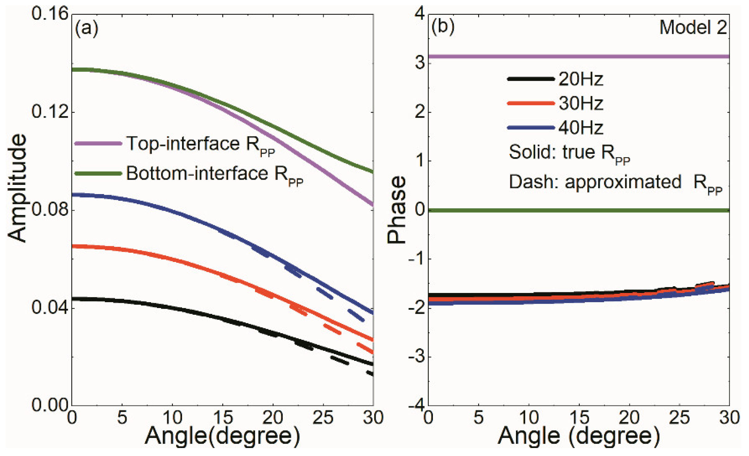Meanwhile, we plot relative errors of R_PP induced by the approximate formula under the small-incidence assumption for Models 1–4 in Figure 8. Considering small-incidence assumption of the approximate formula, the maximum incidence angle in all cases is set as 30 degrees. Due to that thin-bed R_PP are complex valued, we discuss them in terms of amplitude and phase components, respectively.

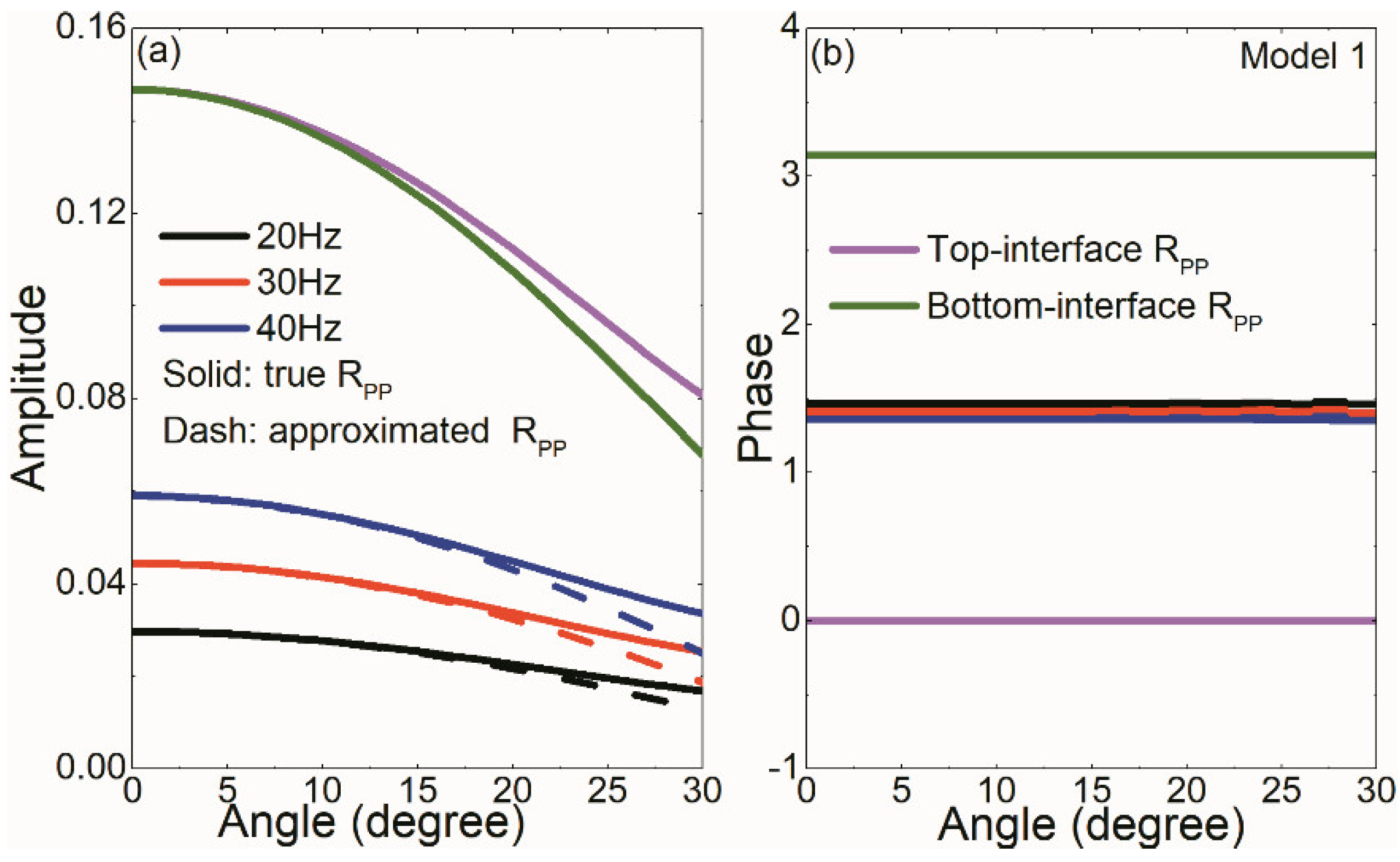
Figure 4 and Figure 5 show R_PP of Models 1 and 2 versus incidence angles, respectively. Models 1 and 2 are high-impedance or low-impedance thin beds with strong impedance contrasts. Destructive interference effects cause that thin-bed reflected amplitudes are obviously lower than those of top- and bottom-interfaces. Meanwhile, the thin-bed reflected phases are not constant zero or π as those of top- and bottom-interfaces, respectively. Compared with the true R_PP, the approximated values show a similar change regularity that a larger incidence angle and a lower incidence frequency result in a lower reflected amplitude. For incidence angles smaller than 20 degrees, approximate thin-bed amplitudes are almost the same as the true values. When incidence angles are over 20 degrees, the approximate thin-bed amplitudes are lower than the true values and show a larger deviation from the true values at a larger incidence angle. The approximated phase is almost the same as the true phase in the angle range from 0 to 30 degrees.

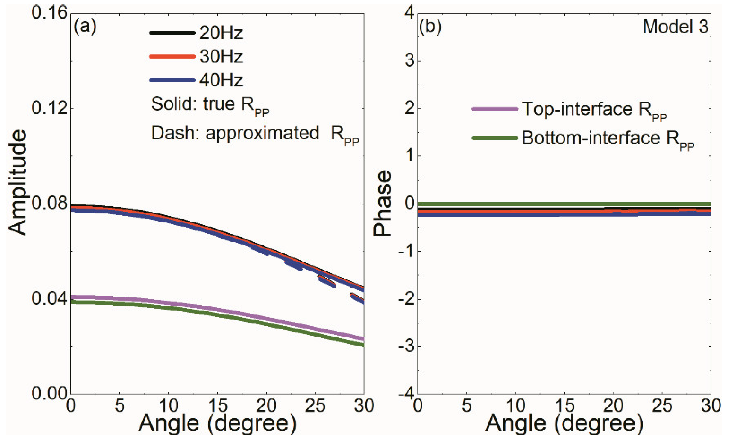
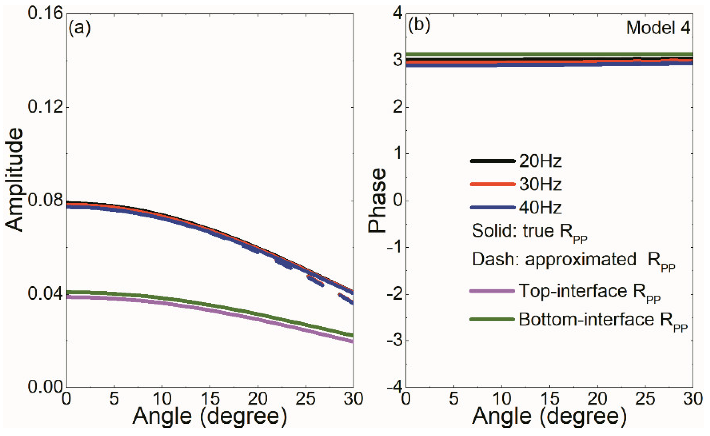
Figure 6 and Figure 7 show R_PP of Models 3 and 4 versus incidence angles, respectively. Models 3 and 4 are impedance transition thin beds with equal polarities, which differ from opposite polarities of Models 1–2. Constructive interference effects cause that thin-bed reflected amplitudes are higher than those of top- and bottom-interfaces. Compared with Models 1–2 cases, R_PP’s amplitudes of Models 3 and 4 are less sensitive to frequency variation. The approximate Amplitude-Versus-Angle (AVA) curves coincide with the true AVA curves for incidence angles smaller than 20 degrees and deviate progressively from the true for incidence angles over 20 degrees. Comparison of Models 3 and 4 shows that the former’s phases are nearly zero while these of the latter are nearly π.

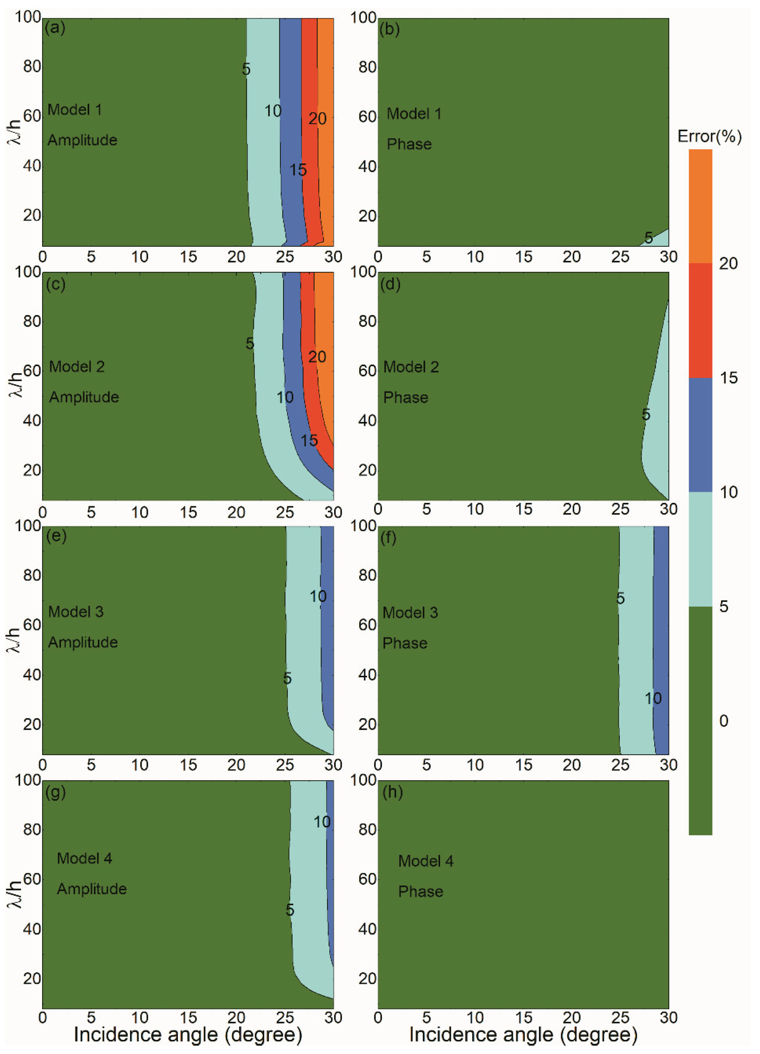
Figure 8 shows R_PP’s relative errors caused by the approximate formula under the small-incidence assumption. In the numerical analysis, thin-bed thickness varies from λ/100 to λ/8, where λ is the P-wave wavelength in the middle layer. Approximate amplitude errors of Models 1–2 are less than 5% for incidence angles smaller than 20 degrees, and are less than 10% for incidence angles less than 25 degrees. When incidence angles are over 25 degrees, amplitude errors increase rapidly with an incidence-angle increase. Phase errors are less than 10% for incidence angles smaller than 30 degrees. For Models 3 and 4, amplitude accuracy by the approximate formula is higher than those of Models 1–2. Approximate errors of Model 3 are less than 5% for incidence angles smaller than 25 degrees and are less than 10% for incidence angles smaller than 29 degrees. For Model 4, amplitude errors versus incidence angles have similar variation regularity with those of Model 3, while, phase errors are smaller than 5% for incidence angles less than or equal to 30 degrees.

To sum up, thin-bed R_PP are significantly different from the top- or bottom-interface R_PP calculated by the Zoeppritz equations. The second-order series approximation has high accuracy for incidence angles less than 20 degrees and deviates progressively from the true values over 20 degrees. Correspondingly, the relative errors are less than 5% for incidence smaller than 20 degrees.

5. Application Example

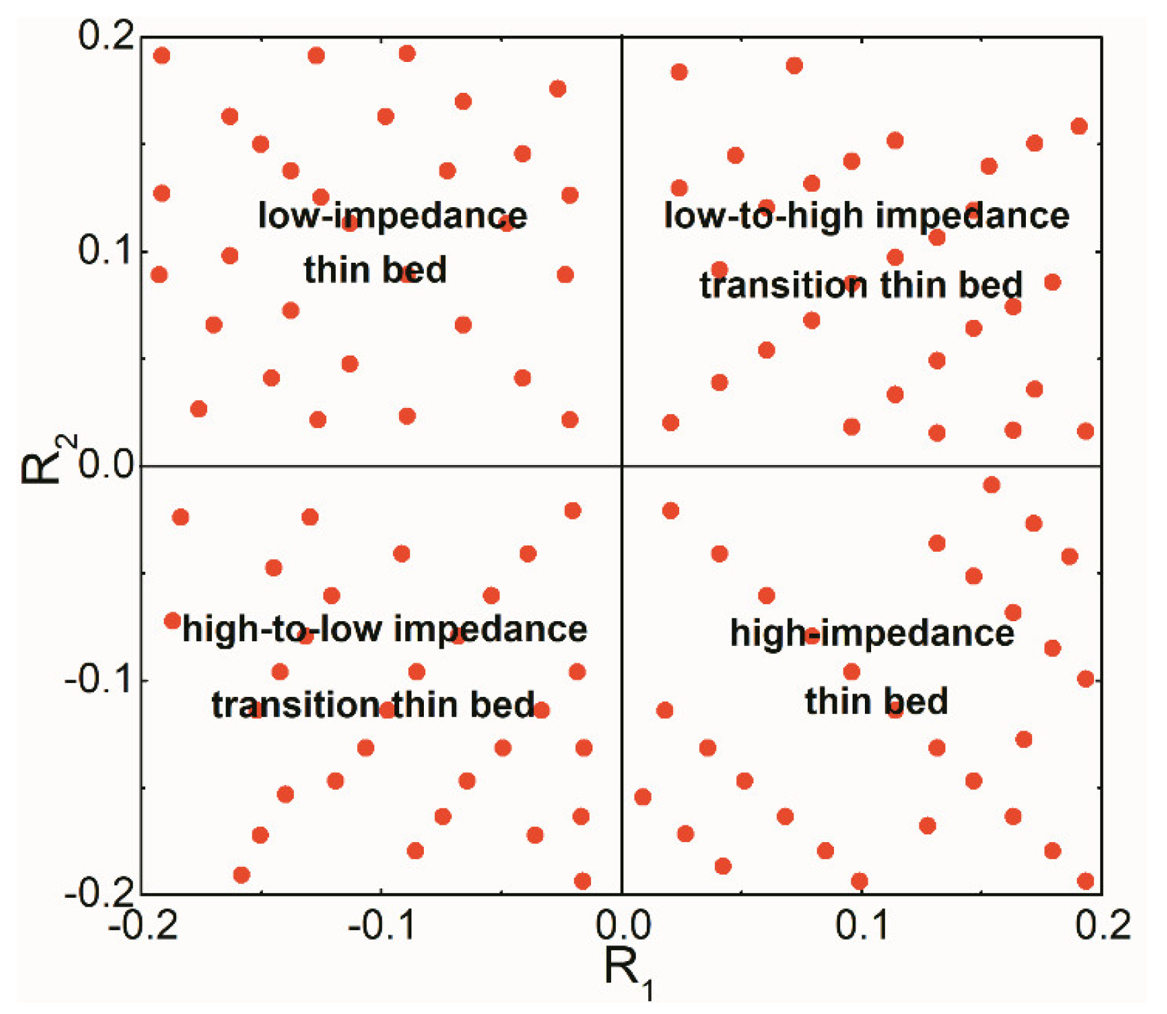
Using the second-order series approximation, we built templates to estimate thin-bed properties, including P-wave impedance ratios and thin-bed thickness. The templates are constituted by amplitude and phase contour maps of R_PP’s A₀, A₂ of 120 thin-bed models. Figure 9 shows the R₁ and R₂ distributions of 120 thin-bed models, which reveal that those 120 models include most of the cases for thin-bed R₁ and R₂ ranging from −0.2 to 0.2. Meanwhile, those 120 models cover all types of thin-bed models, i.e., high-impedance thin beds, low-impedance thin beds, high-to-low impedance transition thin beds and low-to-high impedance transition thin beds, of which each type includes 30 models.

The thin-bed thickness of those 120 models is set as λ/10, λ/20, λ/30, λ/40, λ/50, λ/60, λ/70, λ/80, λ/90, and λ/100. Using the second-order series approximation, we plot amplitudes and phases contour maps of R_PP’s A₀, A₂ of those 120 thin-beds at different R₁, R₂ and thicknesses. Taking the cases of λ/10, λ/20, λ/40, and λ/60 for examples, the contour maps of A₀ and A₂ of those 120 thin-bed models are shown in Figure 10, Figure 11, Figure 12 and Figure 13 respectively. Considering that the coefficients A₀ and A₂ are also complex valued, we discuss them in terms of amplitude and phase components, respectively. The expressions of amplitude and phase of A₀ and A₂ are shown in Appendix D in detail.

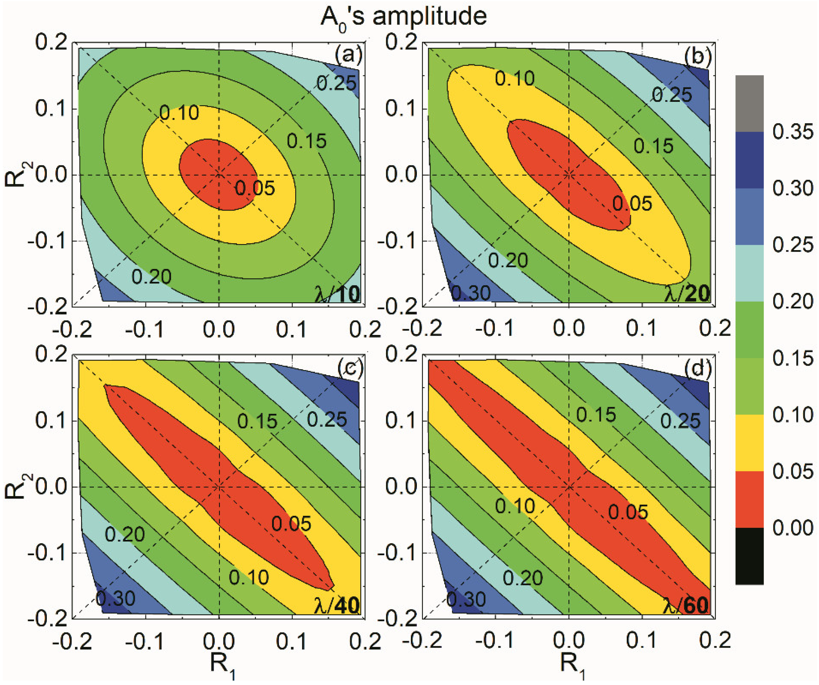
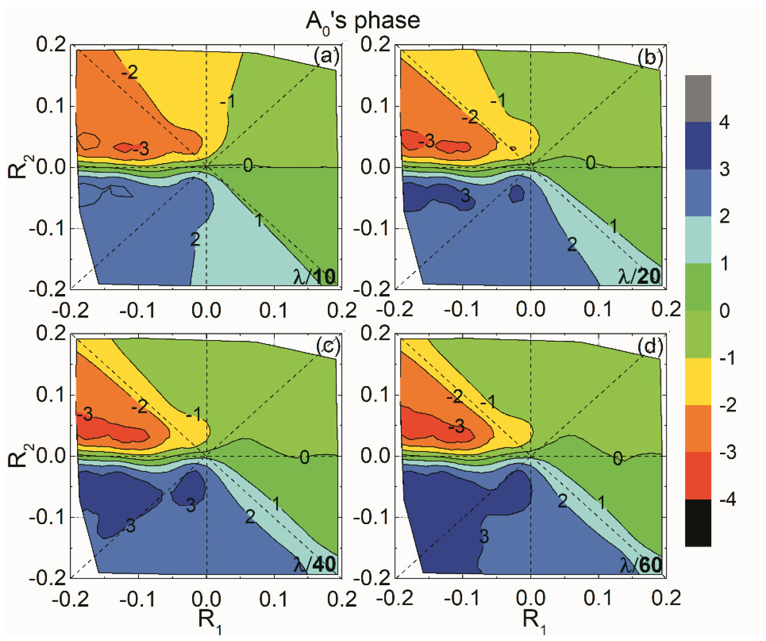
Figure 10 and Figure 11 show A₀’s amplitude and phase of those 120 models versus R₁ and R₂, respectively. For the λ/10 case, amplitude contours are similar to ellipses with the major axis along the line R₂ = −R₁ and minor axis along the line R₂ = R₁. The amplitude increases with increasing R₁ and R₂. The amplitude growth rate of thin-bed models with equal polarities is larger than opposite-polarity cases, especially for a thinner bed. For the cases of thin beds with higher R₁, R₂ and thinner thickness, the amplitude contours in the direction of major axis are approximately parallel to the line R₂ = −R₁. A₀’s phases show that a positive R₂ results in a negative phase, while a negative R₂ results in a positive phase. For the same R₂, a positive R₁ results in a relatively smaller phase than that of a negative R₁ case.

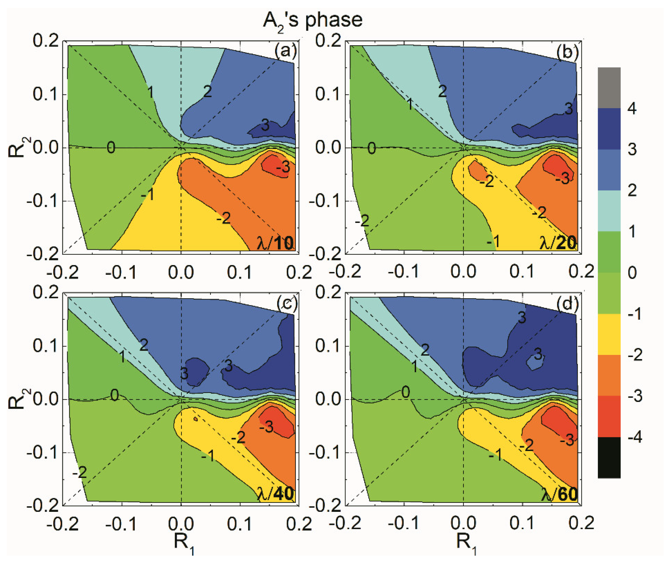
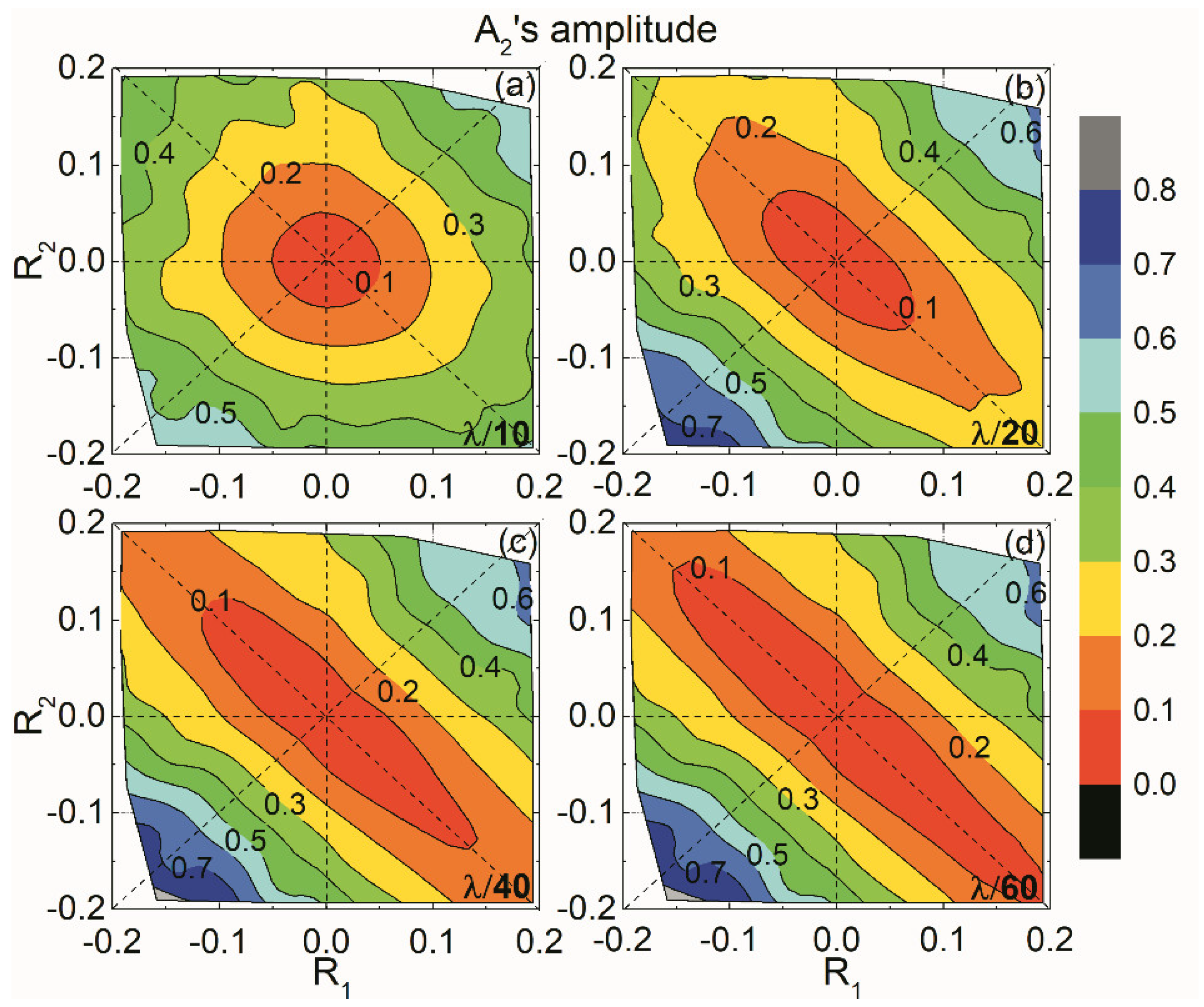
Figure 12 and Figure 13 show A₂’s amplitude and phase of those 120 models versus R₁ and R₂, respectively. Compared with A₀, A₂ has a relatively higher amplitude and a completely different phase variation. For A₂, a positive R₂ results in a positive phase, while a negative R₂ results in a negative phase.

When thin-bed R₁ and R₂ range from −0.2 to 0.2, thin-bed properties can be estimated based on the templates of A₀ and A₂. Once the amplitude and phase values of A₀ and A₂ are obtained from thin-bed AVA data, we can exhibit the corresponding contours in the templates and seek the intersections of those contours. The intersection of the four contour curves, including those of amplitude and phase of A₀ and A₂, indicates thin-bed R₁, R₂ and thickness. The P-wave impedance ratios at the top- and bottom-interfaces of the thin bed can be obtained from R₁, R₂ as follows,

$$\frac{z_{P2}}{z_{P1}}=\frac{1+R_1}{1-R_1}$$

(12)

and

$$\frac{z_{P3}}{z_{P2}}=\frac{1+R_2}{1-R_2}$$

(13)

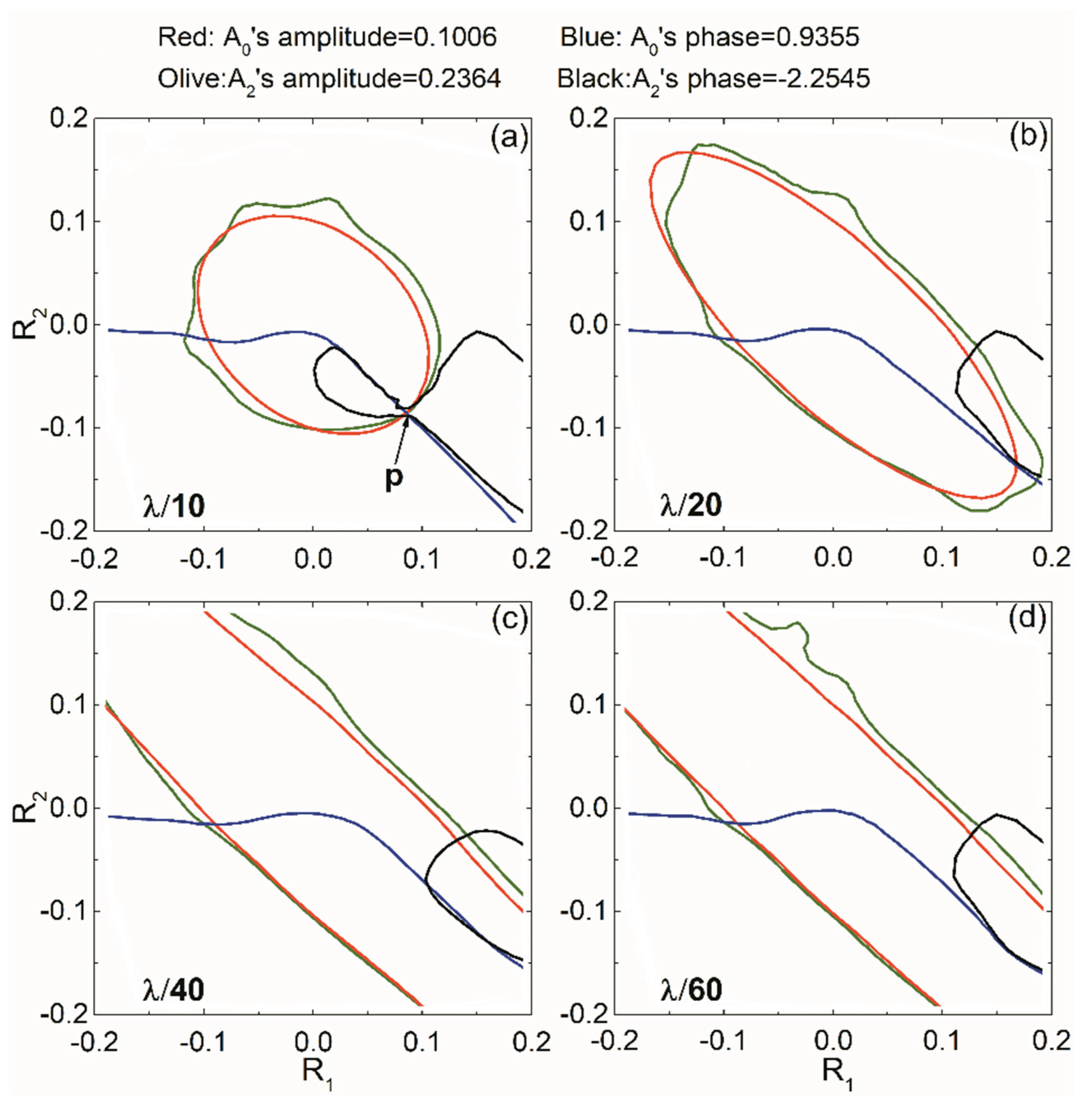
In order to illustrate the estimation approach clearly, we build up a testing thin-bed model, marked as Model 5, whose parameters are listed in

Table 2. Rock properties, A₀ and A₂ of the testing thin-bed model, units of velocities and densities are m/s and g/cm³, respectively.

	Layer No.	vP	vS	ρ	h	R1	R2
Model 5	1	3000	1414	2.29	/	/	/
	2	3440	1793	2.37	λ/10	0.0854	−0.0854
	3	3000	1414	2.29	/	/	/
	A0	Amplitude	0.1006	A2		Amplitude	0.2364
		Phase	0.9355			Phase	−2.2545

. For Model 5, amplitude and phase of A₀ are 0.1006 and 0.9355 respectively, amplitude and phase of A₂ are 0.2364 and −2.2545 respectively. We obtain the corresponding contour lines in the amplitude and phase templates at different thicknesses. Taking the cases of λ/10, λ/20, λ/40, and λ/60 for examples, we exhibit the contours lines of amplitude and phase of A₀ and A₂ at fixed thicknesses, which are shown in Figure 14.

In Figure 14, the four contour curves intersect at a point “p” approximately when the thin-bed thickness is equal to λ/10. While there is no common intersect of the four contour curves for the other thickness cases. Therefore, we estimate the thin-bed thickness is equal to λ/10, which is consistent with the true value (λ/10). R₁ and R₂ are estimated through the coordinates of the intersect point “p”, as R₁ = 0.087 and R₂ = −0.085. The estimated R₁ and R₂ are very close to those of Model 5 (R₁ = 0.085, R₂ = −0.085) respectively. Meanwhile, the estimated P-wave impedance ratios at the top- and bottom-interfaces are 1.190 and 0.843, of which the relative errors are 0.32% and 0.08%, respectively. The good estimated results verify the availability of the estimation approach for thin-bed properties based on the approximate formula.

6. Discussion

Utilizing the parity of trigonometric functions in the exact displacement R/T matrix equations, P- and S-wave R/T coefficients are expressed in form of power series functions of sine incidence angles. Considering the factor that P-wave reflection responses are broadly used at present, we just give the second-order series approximation of thin-bed P-wave reflection coefficients. If necessary, the approximate formula of P-S reflection coefficients can be given through the similar approximate method.

This paper concentrates on the derivation of R_PP’s approximate formula of a single thin bed. When the target thin bed is embedded in a finely layered background, the reflection problems become much more complex. The study shows that interlayer structure and lithologies of finely layered reservoirs can be determined by long-wavelength approximation [37,38,39,40]. Therefore, we will introduce long-wavelength approximation in our further AVA analysis and inversion of finely layered reservoirs.

Thin-bed properties estimation in Section 5 is just an example of the application of the approximate formula for thin-bed properties analysis. In this paper, we give the templates to estimate thin-bed properties based on A₀, A₂ from 120 thin-bed models with R₁ and R₂ between −0.2 and 0.2. Meanwhile, the S-wave velocity and density of those 120 thin-bed models are determined by P-wave velocity through Castagna’s Relationship [41] and Gardner’s Equation [42], respectively. We will develop the database of templates gradually for a wider application in future thin-bed properties analysis.

7. Conclusions

Based on the exact displacement R/T matrix equations of a thin bed, this paper first expands thin-bed R/T coefficients in the form of a power series of sine incidence angles. P-wave R/T coefficients are even functions of sine incidence angles, while S-wave R/T coefficients are odd functions. Under the small-incidence assumption, P-wave reflection coefficients are simplified into the second-order series approximation of sine incidence angles. Meanwhile, it is worthy to notice that, the approximate formula is also based on the fundamental assumptions of conventional AVO methods, including horizontal interface, incident plane-wave, continuous boundary conditions, etc.

Numerical analysis shows the approximate formula of thin-bed R_PP can reveal the thin-bed true reflections for small incidence exactly. Relative errors are less than 5% for incidence angles smaller than 20 degrees. The approximate formula is derived with no weak impedance contrast hypothesis, so it is valid for thin-bed models with strong impedance contrasts. The proposed approach to estimate thin-bed properties is established by thin-bed models with R₁ and R₂ between −0.2 and 0.2. The templates of amplitude and phase of A₀, A₂ can be utilized to estimate P-wave impedance ratios and thin-bed thickness, which verify the availability of the approximate formula.