Grouting Process Simulation Based on 3D Fracture Network Considering Fluid–Structure Interaction

Abstract
:1. Introduction
2. Methodology
2.1. Modeling of 3D Fracture Network
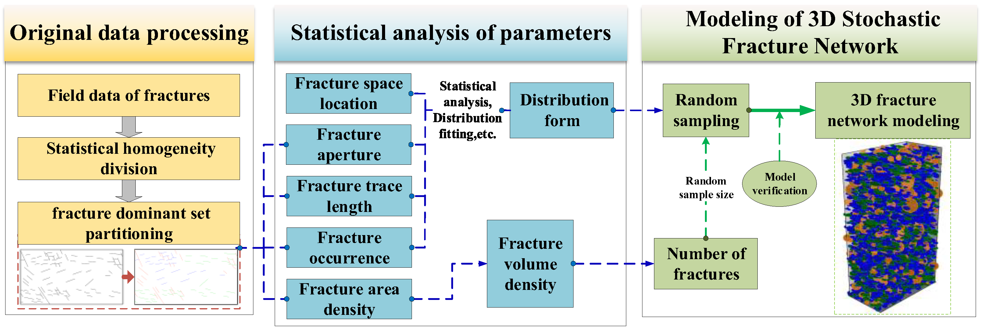
2.1.1. Modeling Process of 3D Fracture Network
2.1.2. Statistical Analysis of Fracture Geometric Characteristic Parameters
- (1)
- Fracture space locationThe Poisson process [31] is widely used to describe fracture location. The fractures are mutually independent and the uniform distribution function are adopted to obtain the coordinates (x0, y0, z0) of the fracture center point.
- (2)
- Fracture densityThe Mauldon method [32] is adopted to estimate the fracture volume density. The following equation is used to estimate the trace area density:where λa is the trace area density, n1 is the number of traces which one end can be observed, n2 is the number of traces which both end can be observed, W is the width of rectangular window, H is the height of rectangular window. Then, Equation (4) is adopted to obtain the fracture volume density:where λv is the fracture volume density, D is the fracture diameter, sinν is the sine value of the dip.
- (3)
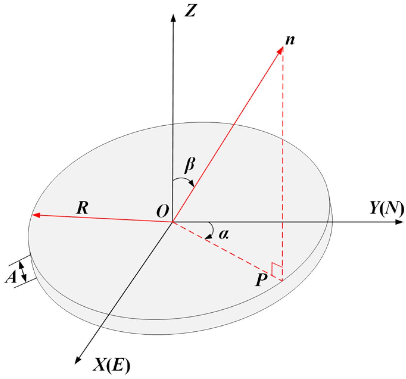
- Fracture sizeTo simulate the size of the fracture surface, statistical analysis of the fracture trace length is needed first. Huang et al. [33] put forward the estimation formula of trace length:where l is the fracture trace length in the window, n0 is the number of traces which neither end can be observed, n1 is the number of traces which one end can be observed, N is the total number of fracture traces in the window, W is the width of rectangular window, H is the height of rectangular window.When the disc model is used to simulate the fracture, the fracture size is expressed by its diameter. the fracture diameter distribution can be confirmed based on the distribution of trace length.
- (4)
- Fracture occurrenceAccording to Kemeny and Post [34], the fisher distribution can be used to fit fracture occurrence and obtained relatively better results.
- (5)
- Fracture aperture
2.1.3. Latin Hypercube Sampling (LHS) Random Sampling
2.2. Fluid–Structure Interaction Model
2.2.1. Computational Fluid Dynamics (CFD) Grouting Numerical Model
- (1)
- The two-phase VOF equationIn the process of grouting, the grout drives out air or groundwater, which should be treated as a two-phase flow [4]. The accurate description of the interface between two kinds of incompatible and incompressible fluids is one of the most important issues in multi-fluid flow computations [39], this can be solved by the VOF method which is proposed by Hirt and Nichols [40] to track free fluid surfaces under fixed grid condition. Therefore, the VOF method is used to keep track of the grout-air interface in this paper. In this method, a volume fractional variable F = F (x, y, z, t) for each phase of the model in the computational domain is introduced. Fg = 1 indicates that the volume is occupied by grout while Fg = 0 indicates that the volume contains no grout and is in the air phase, and 0 < Fg < 1 stands for the volume that contains both grout and air. Equation (7) is used to describe the motion of the grout-air interface:where Fg is the volume fraction of grout; ρ is the density of fluid in kg/m3; ν is the kinematic viscosity of fluid in m2/s.
- (2)
- The continuity equation:where ρ is the density of fluid in kg/m3; t is the time in s; u is the velocity of the unit section in m/s.
- (3)
- The momentum equation:where p is the pressure on the fluid micro-unit in Pa, g is the acceleration of gravity in m/s2; η is the apparent viscosity of fluid in Pa·s; the relationship between ν and η is ν = η/ρ; is the shear rate in 1/s, Fst is the surface tension force in N/m3 and is presented as Equation (10) [41]; and S is the momentum resistance source term in N/m3, including inertia loss term Si and viscosity loss term Sν; in this paper, Si can be neglected because of the low velocity of the grout and S = Sν. Equation (11) is the expression of the viscosity loss term Sν:where Fi is the volume fraction of phases; σ is the surface tension coefficient in N/m.where is the viscous drag coefficient and its expression is as follows:where K is the permeability coefficient.In order to obtain single set of equations, ρ and ν in Equations (7)–(12) are no longer constants but are variables weighted by the volume fraction of fluid [42]:where ρg, ρa, νg, νa are the density of grout, the density of air, the kinematic viscosity of grout and the kinematic viscosity of air, respectively.
- (4)
- The Papanastasiou regularized equationThe cement grout with a w/c ratio of less than 1 is usually described by the Bingham model. However, in the Bingham constitutive equation, when the shear rate is close to zero, the apparent viscosity will become infinite, which causes problems in numerical simulation. In order to solve this problem, the Papanastasiou regularized model is used to describe the rheological properties of cement grout [4], as shown in Equation (15):where η is the apparent viscosity of fluid in Pa·s; m is the stress growth parameter in s; τ0 is the yield stress in Pa; is the shear rate in 1/s; η0 represents the plastic viscosity in Pa·s; and e is a natural constant. From our previous research [4], it is considered that m = 100 can meet the research needs and can make the numerical model effectively express the rheological properties of cement grout.
2.2.2. Computational Structure Dynamics (CSD) Model
2.2.3. Fluid–Structure Interaction Analysis Solution
2.2.4. Boundary Conditions
- (1)
- Inlet boundary conditions: according to the data of grouting pressure measured by grouting recorder and taking the mean value of grouting pressure during grouting period, pressure inlet is set at the boundary of grouting borehole interval. The corresponding grout VOF at the inlet is set to 1.
- (2)
- Outlet boundary conditions: the pressure outlet is set at the end boundary of the fracture, and the pressure satisfies the second boundary condition.
- (3)
- Initial conditions: assuming that there is no groundwater during grouting, the fractures are filled with air before grouting, and the initial air VOF in the fracture is set to 1.
- (4)
- Displacement boundary conditions: the bottom boundary of the computational domain is the z-axis constraint, the lateral boundaries are the x- and y-axis constraints.
3. Case Study
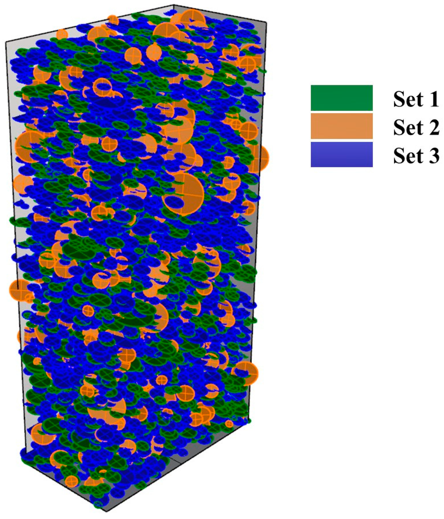
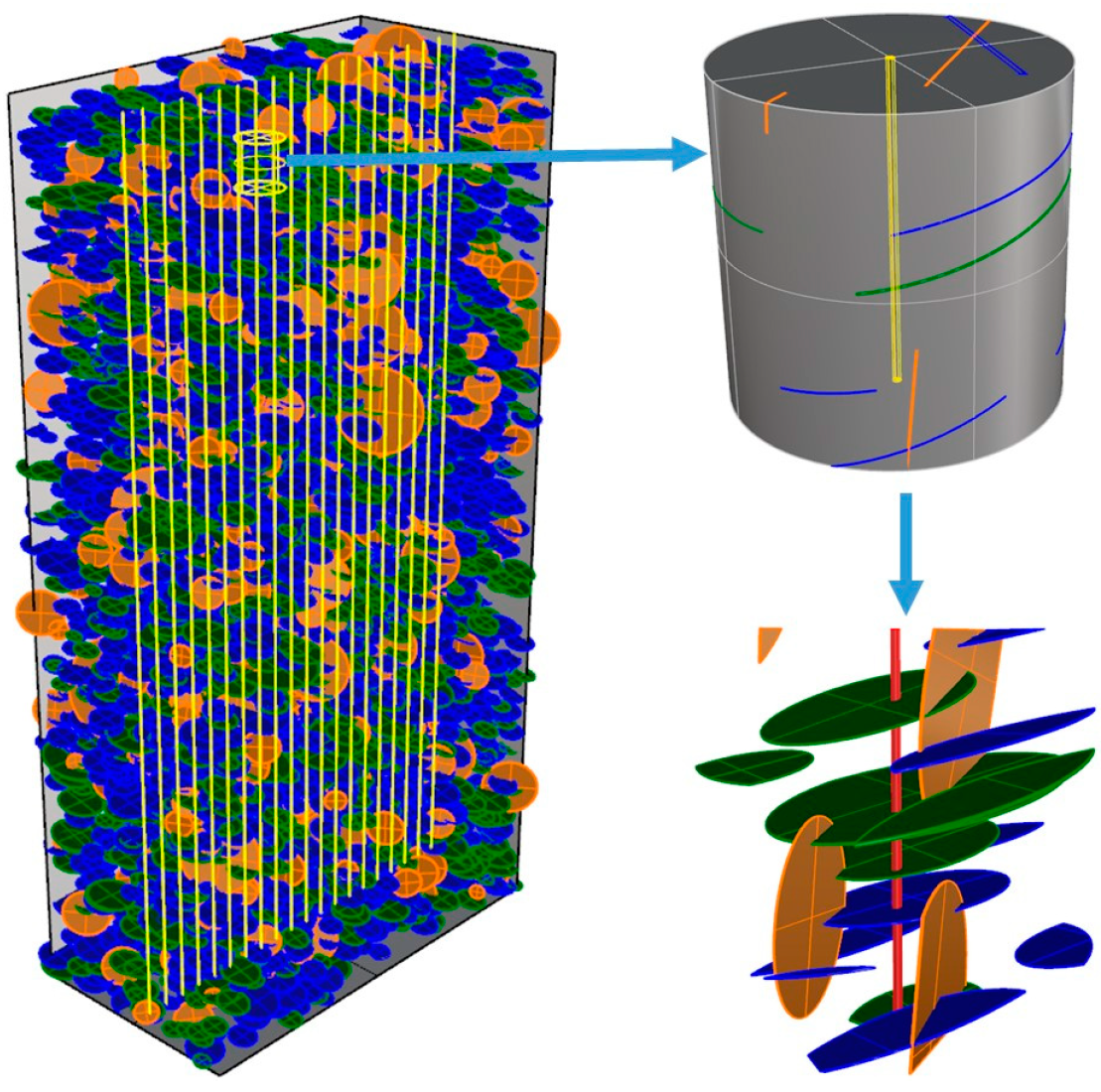
3.1. Simulation of 3D Fracture Network
3.2. Grouting Simulation Considering Fluid–Structure Interaction
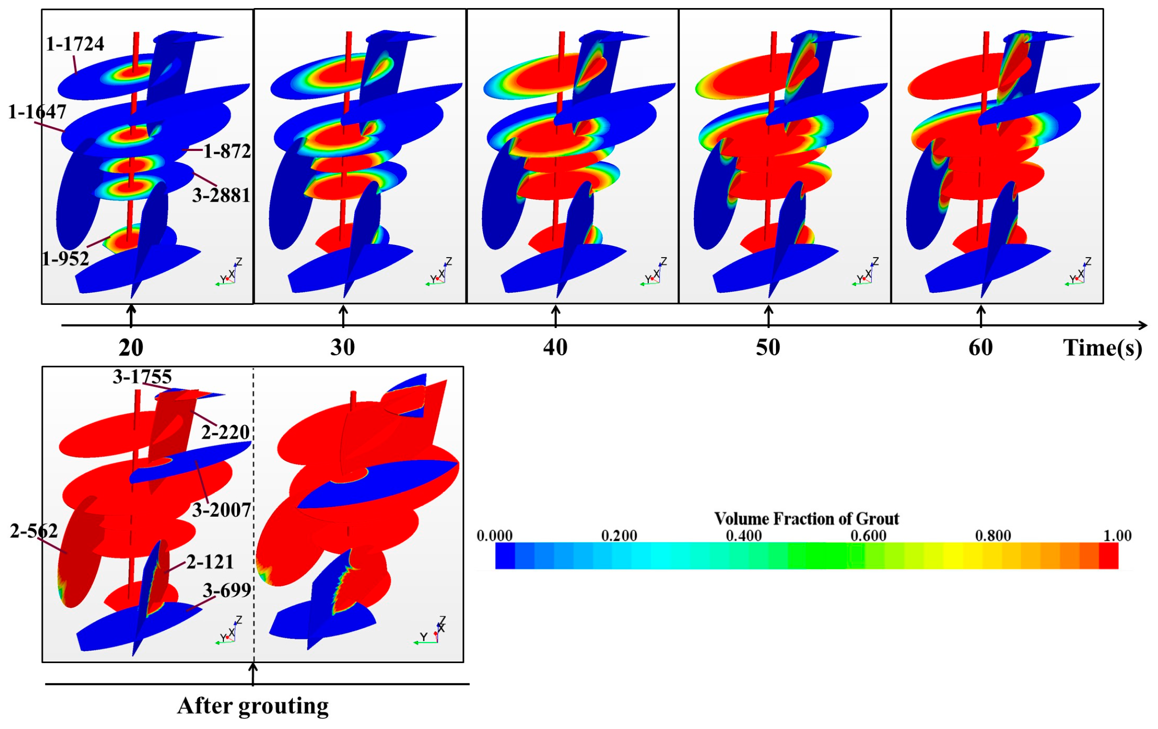
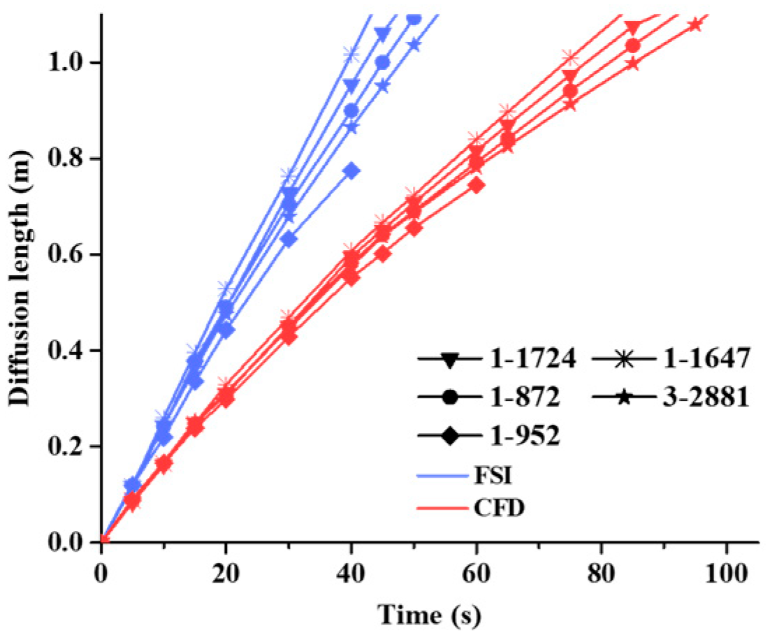
3.2.1. Analysis of Fluid Calculation
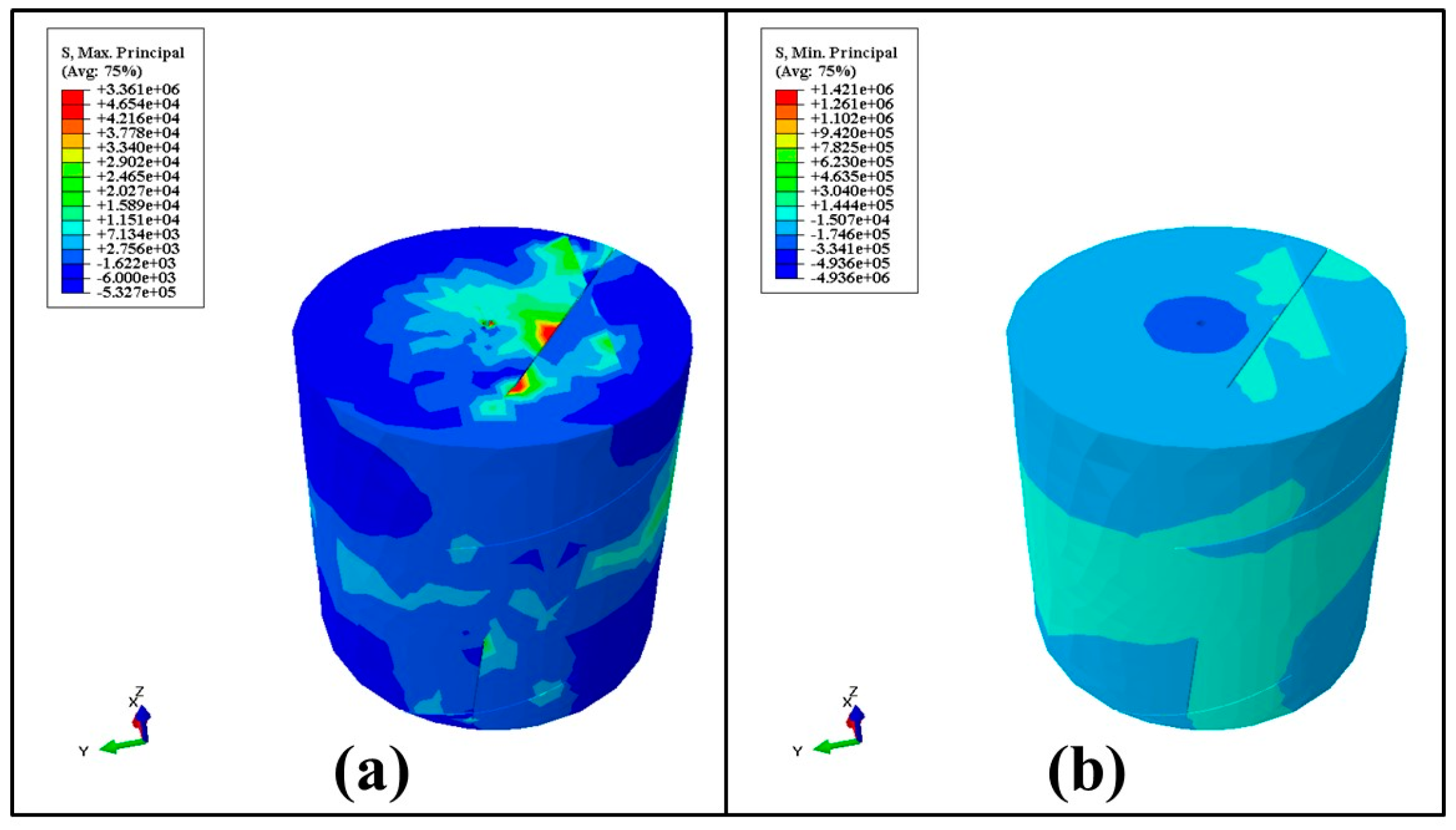
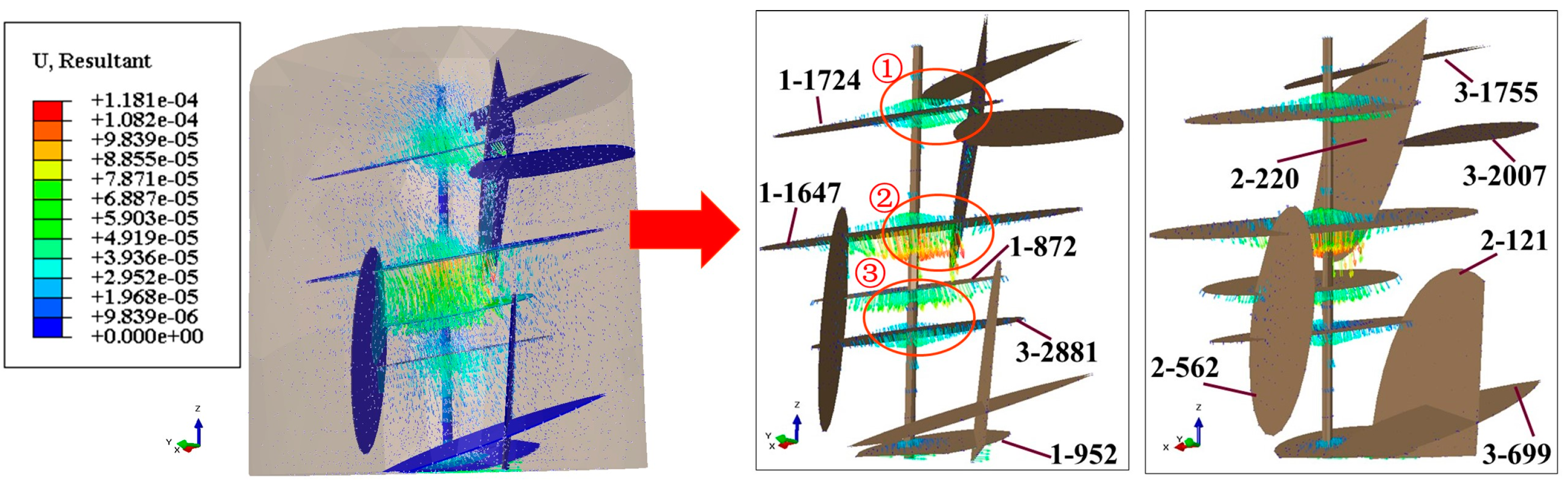
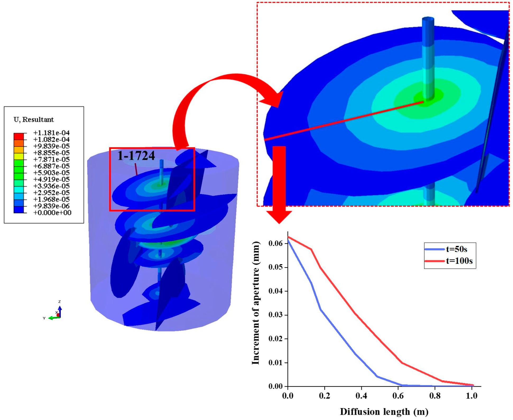
3.2.2. Analysis of Structural Calculation
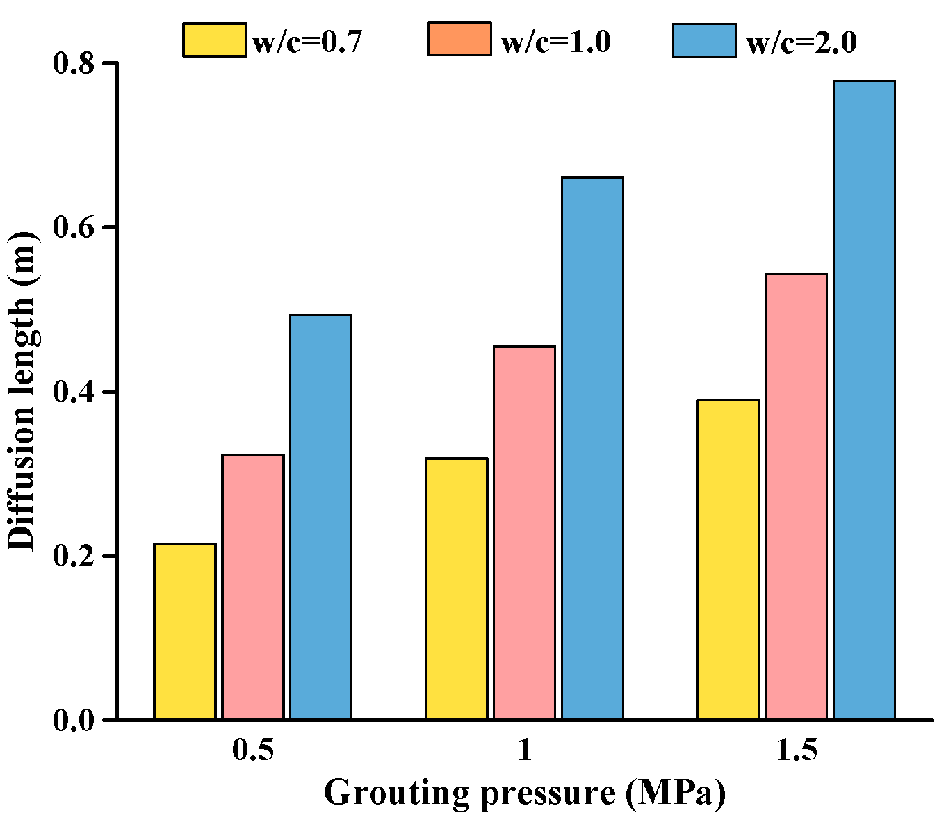
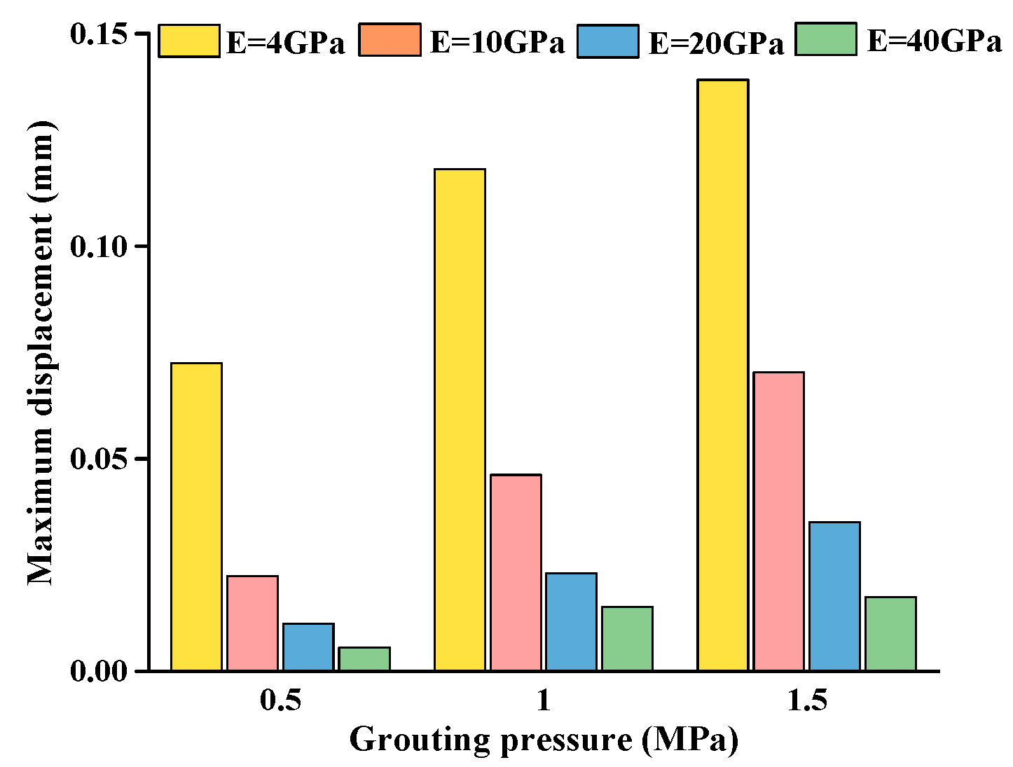
3.3. Parameter Analysis
4. Conclusions
- (1)
- In fracture network modeling studies, fracture aperture values are often ignored or inaccurate, which will affect the authenticity of grout simulation. Combined with the exposed surface fracture catalog data, we use the relationship between fracture apertures and trace lengths to obtain a more realistic value of fracture aperture and to establish a more reliable model for numerical simulation of grouting.
- (2)
- During the grouting process, the filling of the primary fractures is influenced by the number of intersecting secondary fractures, whilst the filling of the secondary fractures is related to the fracture aperture, and the length of the intersection between the secondary facture and the primary fracture. Fracture aperture and dip angle have a significant effect on the grout diffusion rate, while the fracture aperture is the major influencing factor. Moreover, the effect of fluid–structure interaction between the grout flow and the rock mass has a certain influence on the grout diffusion length and neglecting this effect will cause an underestimation of the grouting performance.
- (3)
- When the fractures in a certain region intersect with each other and are close to other fractures in the surrounding area, the rock mass between such fractures will be the least rigid and prone to deformation during the grouting process.
- (4)
- Grouting pressure, grout water–cement ratio and rock mass elastic module all have effects on the grouting process. Therefore, in the grouting construction process, the appropriate grouting pressure and grout water–cement ratio should be selected according to different geological conditions.
- (5)
- The effects of fluid–structure interaction between the grout and the rock mass will affect the grout diffusion process and the rock mass deformation. Therefore, the grouting process simulation considering the fluid–structure interaction can better analyze grout diffusion and rock deformation, and hence explore the grouting mechanism under real conditions.
Author Contributions
Funding
Conflicts of Interest
References
- Saeidi, O.; Azadmehr, A.; Torabi, S.R. Development of a rock groutability index based on the rock engineering systems (res): A case study. Indian Geotech. J. 2014, 44, 49–58. [Google Scholar] [CrossRef]
- Lin, P.; Zhu, X.X.; Li, Q.B.; Liu, H.Y.; Yu, Y.J. Study on Optimal Grouting Timing for Controlling Uplift Deformation of a Super High Arch Dam. Rock Mech. Rock Eng. 2016, 49, 115–142. [Google Scholar] [CrossRef]
- Mohajerani, S.; Baghbanan, A.; Wang, G.; Forouhandeh, S.F. An Efficient Algorithm for Simulating Grout Propagation in 2D Discrete Fracture Networks. Int. J. Rock Mech. Min. Sci. 2017, 98, 67–77. [Google Scholar] [CrossRef]
- Deng, S.H.; Wang, X.L.; Yu, J.; Zhang, Y.C.; Liu, Z.; Zhu, Y.S. Simulation of grouting process in rock masses under a dam foundation characterized by a 3D fracture network. Rock Mech. Rock Eng. 2018, 51, 1801–1822. [Google Scholar] [CrossRef]
- Saeidi, O.; Håkan, S.; Torabi, S.R. Numerical and analytical analyses of the effects of different joint and grout properties on the rock mass groutability. Tunn. Undergr. Space Technol. 2013, 38, 11–25. [Google Scholar] [CrossRef]
- Yang, P.; Sun, X.Q. Single fracture grouting numerical simulation based on fracture roughness in hydrodynamic environment. Electron. J. Geotechn. Eng. 2015, 20, 59–67. [Google Scholar]
- Fu, P.; Zhang, J.J.; Xing, Z.Q.; Yang, X.D. Numerical Simulation and Optimization of Hole Spacing for Cement Grouting in Rocks. J. Appl. Math. 2013, 2013, 1–9. [Google Scholar] [CrossRef]
- Hao, M.M.; Wang, F.M.; Li, X.L.; Zhang, B.; Zhong, Y.H. Numerical and experimental studies of diffusion law of grouting with expansible polymer. J. Mater. Civ. Eng. 2018, 30, 04017290. [Google Scholar] [CrossRef]
- Kim, H.M.; Lee, J.W.; Yazdani, M.; Tohidi, E.; Nejati, H.R.; Park, E.S. Coupled Viscous Fluid Flow and Joint Deformation Analysis for Grout Injection in a Rock Joint. Rock Mech. Rock Eng. 2018, 51, 627–638. [Google Scholar] [CrossRef]
- Ao, X.F.; Wang, X.L.; Zhu, X.B.; Zhou, Z.Y.; Zhang, X.X. Grouting simulation and stability analysis of coal mine goaf considering hydromechanical coupling. J. Comput. Civ. Eng. 2017, 31, 04016069. [Google Scholar] [CrossRef]
- Liu, Q.S.; Sun, L. Simulation of coupled hydro-mechanical interactions during grouting process in fractured media based on the combined finite-discrete element method. Tunn. Undergr. Space Technol. 2019, 84, 472–486. [Google Scholar] [CrossRef]
- Berrone, S.; Canuto, C.; Pieraccini, S.; Scialò, S. Uncertainty quantification in discrete fracture network models: Stochastic fracture transmissivity. Comput. Math. Appl. 2015, 70, 603–623. [Google Scholar] [CrossRef]
- Li, M.C.; Han, S.; Zhou, S.B.; Zhang, Y. An Improved Computing Method for 3D Mechanical Connectivity Rates Based on a Polyhedral Simulation Model of Discrete Fracture Network in Rock Masses. Rock Mech. Rock Eng. 2018, 51, 1789–1800. [Google Scholar] [CrossRef]
- Han, X.D.; Chen, J.P.; Wang, Q.; Li, Y.Y.; Zhang, W.; Yu, T.W. A 3D Fracture Network Model for the Undisturbed Rock Mass at the Songta Dam Site Based on Small Samples. Rock Mech. Rock Eng. 2016, 49, 611–619. [Google Scholar] [CrossRef]
- Yan, C.Z.; Zheng, H. Three-dimensional hydromechanical model of hydraulic fracturing with arbitrarily discrete fracture networks using finite-discrete element method. Int. J. Geomech. 2016, 17, 04016133. [Google Scholar] [CrossRef]
- Shiriyev, J. Discrete Fracture Network Modeling in a Carbon Dioxide Flooded Heavy Oil Reservoir. Master’s Thesis, Middle East Technical University, Ankara, Turkey, 2014. [Google Scholar]
- Schultz, R.A.; Soliva, R.; Fossen, H.; Okubo, C.H.; Reeves, D.M. Dependence of displacement–length scaling relations for fractures and deformation bands on the volumetric changes across them. J. Struct. Geol. 2008, 30, 1405–1411. [Google Scholar] [CrossRef]
- Schultz, R.A.; Klimczak, C.; Fossen, H.; Olson, J.E.; Exner, U.; Reeves, D.M.; Soliva, R. Statistical tests of scaling relationships for geologic structures. J. Struct. Geol. 2013, 48, 85–94. [Google Scholar] [CrossRef]
- Liu, R.C.; Li, B.; Jiang, Y.J.; Huang, N. Review: Mathematical expressions for estimating equivalent permeability of rock fracture networks. Hydrogeol. J. 2016, 24, 1623–1649. [Google Scholar] [CrossRef]
- Klimczak, C.; Schultz, R.A.; Parashar, R.; Reeves, D.M. Cubic law with aperture-length correlation: Implications for network scale fluid flow. Hydrogeol. J. 2010, 18, 851–862. [Google Scholar] [CrossRef]
- GothäLl, R.; Stille, H. Fracture–fracture interaction during grouting. Tunn. Undergr. Space Technol. 2010, 25, 199–204. [Google Scholar] [CrossRef]
- Tsang, C.F. Coupled hydromechanical-thermochemical processes in rock fractures. Rev. Geophys. 1991, 29, 537–551. [Google Scholar] [CrossRef]
- Rafi, J.Y.; Stille, H. Control of rock jacking considering spread of grout and grouting pressure. Tunn. Undergr. Space Technol. 2014, 40, 1–15. [Google Scholar] [CrossRef]
- Rafi, J.Y.; Stille, H. Basic mechanism of elastic jacking and impact of fracture aperture change on grout spread, transmissivity and penetrability. Tunn. Undergr. Space Technol. 2015, 49, 174–187. [Google Scholar] [CrossRef]
- Cerroni, D.; Fancellu, L.; Manservisi, S.; Menghini, F. Fluid structure interaction solver coupled with volume of fluid method for two-phase flow simulations. AIP Conf. Proc. 2016, 1738, 030024. [Google Scholar] [CrossRef]
- Chen, J.; Liu, H.; Wang, F.S.; Shi, G.C.; Cao, G.; Wu, H.G. Numerical prediction on volumetric efficiency of progressive cavity pump with fluid–solid interaction model. J. Pet. Sci. Eng. 2013, 109, 12–17. [Google Scholar] [CrossRef]
- Villiers, A.M.D.; Mcbride, A.T.; Reddy, B.D.; Franz, T.; Spottiswoode, B.S. A validated patient-specific FSI model for vascular access in haemodialysis. Biomech. Model. Mech. 2018, 17, 479–497. [Google Scholar] [CrossRef] [PubMed]
- Rabczuk, T.; Gracie, R.; Song, J.H.; Belytschko, T. Immersed particle method for fluid–structure interaction. Int. J. Numer. Meth. Eng. 2010, 81, 48–71. [Google Scholar] [CrossRef]
- Zhong, D.H.; Li, M.C.; Liu, J. 3D integrated modeling approach to geo-engineering objects of hydraulic and hydroelectric projects. Sci. China Ser. E Technol. Sci. 2007, 50, 329–342. [Google Scholar] [CrossRef]
- Baecher, G.B.; Lanney, N.A.; Einstein, H.H. Statistical description of rock properties and sampling. In Proceedings of the 18th US Symposium on Rock Mechanics (USRMS), Golden, Colorado, 22–24 June 1977; American Rock Mechanics Association: Golden, CO, USA, 1977. Available online: https://www.onepetro.org/conference-paper/ARMA-77-0400 (accessed on 29 January 2019).
- Xu, C.S.; Dowd, P. A new computer code for discrete fracture network modelling. Comput. Geosci. 2010, 36, 292–301. [Google Scholar] [CrossRef]
- Mauldon, M. Estimating mean fracture trace length and density from observations in convex windows. Rock Mech. Rock Eng. 1998, 31, 201–216. [Google Scholar] [CrossRef]
- Huang, R.Q.; Xu, M.; Chen, J.P. Meticulous Description of Complex Structure and Its Engineering Application; Science Press: Beijing, China, 2004. [Google Scholar]
- Kemeny, J.; Post, R. Estimating three-dimensional rock discontinuity orientation from digital images of fracture traces. Comput. Geosci. 2003, 29, 65–77. [Google Scholar] [CrossRef]
- Miao, T.J.; Yu, B.; Duan, Y.G.; Fang, Q.T. A fractal analysis of permeability for fractured rocks. Int. J. Heat Mass Transf. 2015, 81, 75–80. [Google Scholar] [CrossRef]
- Xu, S.S.; Nieto-Samaniego, A.F.; Alaniz-Álvarez, S.A.; Velasquillo-Martínez, L.G. Effect of sampling and linkage on fault length and length–displacement relationship. Int. J. Earth Sci. 2006, 95, 841–853. [Google Scholar] [CrossRef]
- Zhu, J.T.; Cheng, Y.Y. Effective permeability of fractal fracture rocks: Significance of turbulent flow and fractal scaling. Int. J. Heat Mass Transf. 2018, 116, 549–556. [Google Scholar] [CrossRef]
- Matthies, H.G.; Niekamp, R.; Steindorf, J. Algorithms for strong coupling procedures. Comput. Methods Appl. Mech. Eng. 2006, 195, 2028–2049. [Google Scholar] [CrossRef]
- Chen, Y.G.; Price, W.G.; Temarel, P. An anti-diffusive volume of fluid method for interfacial fluid flows. Int. J. Numer. Methods Fluids 2012, 68, 341–359. [Google Scholar] [CrossRef]
- Hirt, C.W.; Nichols, B.D. Volume of fuid (VOF) method for the dynamics of free boundaries. J. Comput. Phys. 1981, 39, 201–225. [Google Scholar] [CrossRef]
- STAR-CCM + User Guide Version 10.02. CD-Adapco. 2015. Available online: https://mdx.plm.automation.siemens.com/star-ccm-plus (accessed on 29 January 2019).
- Gopala, V.R.; Wachem, B.G.M.V. Volume of fluid methods for immiscible-fluid and free-surface flows. Chem. Eng. J. 2008, 141, 204–221. [Google Scholar] [CrossRef]
- Giovannetti, L.M.; Banks, J.; Ledri, M.; Turnock, S.R.; Boyd, S.W. Toward the development of a hydrofoil tailored to passively reduce its lift response to fluid load. Ocean Eng. 2018, 167, 1–10. [Google Scholar] [CrossRef]
- Rubio, J.E.; Schilling, P.J.; Chakravarty, U.K. Modal characterization and structural aerodynamic response of a crane fly forewing. Acta Mech. 2018, 229, 2307–2325. [Google Scholar] [CrossRef]
- McVicar, J.; Lavroff, J.; Davis, M.R.; Thomas, G. Fluid–structure interaction simulation of slam-induced bending in large high-speed wave-piercing catamarans. J. Fluids Struct. 2018, 82, 35–58. [Google Scholar] [CrossRef]


| Set | Fracture Number | Regional Volume (m3) | Parameter | Mean | Minimum | Maximum | Distribution |
|---|---|---|---|---|---|---|---|
| 1 | 2587 | 28,800 | Coordinate X/m | 15 | 0 | 30 | Uniform |
| Coordinate Y/m | 8 | 0 | 16 | ||||
| Coordinate Z/m | 30 | 0 | 60 | ||||
| Diameter/m | 1.93 | 0.31 | 2.89 | Lognormal | |||
| Dip direction/degree | 345.00 | 340.00 | 349.98 | Fisher | |||
| Dip angle/degree | 15 | 10.00 | 19.98 |
| Fracture | Coordinate/m | Radius/m | Dip Direction/Deg | Dip Angle/Deg | Aperture/m | ||
|---|---|---|---|---|---|---|---|
| X | Y | Z | |||||
| 1-1724 | 19.874 | 9.182 | 56.403 | 0.835 | 344.432 | 18.027 | 0.0089 |
| 1-1647 | 19.053 | 9.902 | 55.445 | 1.213 | 347.699 | 13.503 | 0.0129 |
| 1-872 | 19.157 | 8.701 | 55.255 | 0.726 | 347.079 | 14.107 | 0.0077 |
| 1-952 | 17.818 | 10.036 | 52.685 | 0.543 | 349.080 | 15.092 | 0.0058 |
| 2-220 | 20.193 | 7.555 | 57.400 | 1.246 | 41.687 | 80.996 | 0.0132 |
| 2-562 | 18.444 | 14.515 | 54.789 | 0.755 | 41.635 | 86.409 | 0.0080 |
| 2-121 | 17.862 | 13.714 | 51.170 | 1.162 | 39.079 | 85.291 | 0.0124 |
| 3-1755 | 18.708 | 7.543 | 56.899 | 1.150 | 9.167 | 14.944 | 0.0122 |
| 3-2007 | 16.190 | 8.332 | 56.259 | 1.099 | 13.901 | 11.962 | 0.0117 |
| 3-2881 | 19.736 | 7.530 | 55.015 | 0.784 | 7.736 | 10.360 | 0.0083 |
| 3-699 | 19.515 | 9.665 | 54.138 | 1.035 | 9.766 | 19.581 | 0.0110 |
| Medium | Density (kg/m3) | Elastic Modulus (MPa) | Poisson Ratio μ | Cohesion C (MPa) | Internal Friction Angle φ (°) |
|---|---|---|---|---|---|
| Slate | 2690 | 4000 | 0.25 | 9.5 | 37.7 |
© 2019 by the authors. Licensee MDPI, Basel, Switzerland. This article is an open access article distributed under the terms and conditions of the Creative Commons Attribution (CC BY) license (http://creativecommons.org/licenses/by/4.0/).
Share and Cite
Zhu, Y.; Wang, X.; Deng, S.; Chen, W.; Shi, Z.; Xue, L.; Lv, M. Grouting Process Simulation Based on 3D Fracture Network Considering Fluid–Structure Interaction. Appl. Sci. 2019, 9, 667. https://doi.org/10.3390/app9040667
Zhu Y, Wang X, Deng S, Chen W, Shi Z, Xue L, Lv M. Grouting Process Simulation Based on 3D Fracture Network Considering Fluid–Structure Interaction. Applied Sciences. 2019; 9(4):667. https://doi.org/10.3390/app9040667
Chicago/Turabian StyleZhu, Yushan, Xiaoling Wang, Shaohui Deng, Wenlong Chen, Zuzhi Shi, Linli Xue, and Mingming Lv. 2019. "Grouting Process Simulation Based on 3D Fracture Network Considering Fluid–Structure Interaction" Applied Sciences 9, no. 4: 667. https://doi.org/10.3390/app9040667
APA StyleZhu, Y., Wang, X., Deng, S., Chen, W., Shi, Z., Xue, L., & Lv, M. (2019). Grouting Process Simulation Based on 3D Fracture Network Considering Fluid–Structure Interaction. Applied Sciences, 9(4), 667. https://doi.org/10.3390/app9040667