A Feature Selection Method for Multi-Label Text Based on Feature Importance

Abstract

Multi-label text classification refers to a text divided into multiple categories simultaneously, which corresponds to a text associated with multiple topics in the real world. The feature space generated by text data has the characteristics of high dimensionality and sparsity. Feature selection is an efficient technology that removes useless and redundant features, reduces the dimension of the feature space, and avoids dimension disaster. A feature selection method for multi-label text based on feature importance is proposed in this paper. Firstly, multi-label texts are transformed into single-label texts using the label assignment method. Secondly, the importance of each feature is calculated using the method based on Category Contribution (CC). Finally, features with higher importance are selected to construct the feature space. In the proposed method, the feature importance is calculated from the perspective of the category, which ensures the selected features have strong category discrimination ability. Specifically, the contributions of the features to each category from two aspects of inter-category and intra-category are calculated, then the importance of the features is obtained with the combination of them. The proposed method is tested on six public data sets and the experimental results are good, which demonstrates the effectiveness of the proposed method.

1. Introduction

With the rapid development of information technology, all walks of life have been generating a large amount of data. Therefore, it is of great significance to promote the development and progress of various industries by mining useful knowledge and information from text data and applying them to information retrieval and data analysis. Text classification is a technology that can effectively organize and manage texts, and facilitate users to quickly obtain useful information, thus becomes an important research direction in the field of information processing.

Text classification refers to a text divided into one or multiple predefined categories according to the content of text data, including single-label text classification and multi-label text classification. In single-label text classification, a text is associated with one predefined topic and only divided into one category [1,2,3]. However, in multi-label text classification, a text is associated with multiple predefined topics and divided into multiple categories [4,5,6]. For example, a news report about a movie may be associated with the topics of “movie”, “music”, and others. Also, an article about computers may be associated with the topics of “computers”, “software engineering”, and others. In the real world, it is very common for a text to be associated with multiple topics, so it is more practical to study multi-label text classification.

Feature selection is an important part of multi-label text classification. Text data is unstructured data, consisting of words. The vector space model is often used to represent text data for facilitating computer processing. In this method, all the terms in all the texts are used as features to construct the feature space which is called the original feature space. Since a text may consist of thousands of different terms, the original feature space is high-dimensional and sparse. If the original feature space is directly used for text classification, it will be time-consuming and over-fitting. Therefore, reducing the dimension of the original feature space is of significant importance. Feature selection is a commonly used dimensionality reduction technology. It removes useless and redundant features, and only keeps the features with strong category discrimination ability to construct the feature subset, realizing the reduction of feature space dimension and the improvement of classification performance [7,8]. We study the feature selection method for multi-label text in this paper.

Currently, there are some researches on feature selection for multi-label data, which can be divided into three categories: wrapped methods, embedded methods, and filter methods. In wrapped methods, several different feature subsets are constructed in advance, the pros and cons of the feature subsets are then evaluated by the predictive precision of the classification algorithm, and the final feature subset is determined based on the evaluation [9,10,11,12,13]. In embedded methods, the feature selection process is integrated into the classification model training process, that is, features with high contribution to model training are selected to construct the feature subset in the process of classification model construction [14,15,16]. In filter methods, the classification contribution of each feature is calculated as its feature importance, and features with higher importance are selected to construct the feature subset [17,18,19,20]. Based on this selected feature subset, the training of the classification model is performed. Therefore, this type of feature selection methods has low computational complexity and high operational efficiency, and is very suitable for text data [21].

In filter methods, the core is how to calculate the feature importance. At present, the commonly used feature importance calculation method is to count the frequency of features in the whole training set. However, the selected features using this method do not necessarily have strong category discrimination ability. For example, the feature “people” appears frequently in the whole training set, so the importance of “people” is very high, calculated by the method of counting its frequency in the whole training set. However, such a feature may appear similar times in each category of the training set, and doesn’t have category discrimination ability indeed. The category discrimination ability of features is an ability to distinguish one category from others. Therefore, the importance of features should be calculated from the perspective of the category discrimination ability. Features with strong category discrimination ability have high correlation with one category and low correlation with others. To the best of our knowledge, there are some researches on the calculation of feature importance based on the two aspects [22,23]. They consider one aspect or two aspects abovementioned, design the feature importance calculation formula, and apply it to single-label text classification. In this paper, on the basis of these researches, the contributions of features to category discrimination are redefined from the above two aspects, and the importance of the features is obtained with the combination of them.

A filter feature selection method for multi-label text is proposed in the paper. Firstly, multi-label texts are transformed into single-label texts using the label assignment method. Secondly, the importance of each feature is calculated using the proposed method of Category Contribution (CC). Finally, features with higher importance are selected to construct the feature space. Thus, the contributions of this paper can be summarized as follows.

(1)

The importance of features for classification is analyzed from two aspects of inter-category and intra-category, and then the formulas for calculating inter-category contribution and intra- category contribution are proposed.

(2)

A formula for calculating feature importance based on CC is proposed.

(3)

The proposed feature selection method is combined with Binary Relevance k-Nearest Neighbor (BRKNN) [24] and Multi-label k-Nearest Neighbor (MLKNN) [25] algorithms, achieving a good classification performance.

The rest of this paper is organized as follows. Section 2 describes some related works. Section 3 introduces the details of the proposed method. Experimental results are shown in Section 4. Finally, Section 5 concludes the findings shown in this paper.

2. Related Works

The purpose of feature selection is to reduce the dimension of the feature space and improve the efficiency and performance of the classification through removing irrelevant and redundant features. The filter feature selection methods are viewed as a pure pre-processing tool and have low computational complexity. As a result, there are many scholars focusing on the research of this type of methods. For multi-label data, there are two main research ideas in filter feature selection methods.

One method is the feature selection method based on the idea of algorithm adaptation. In this type of methods, the feature importance calculation methods commonly used in single-label feature selection are adapted to be suitable for multi-label data, then the feature selection for multi-label data is performed on them [18,19,20,26,27]. Lee et al. [18] proposed a filter multi-label feature selection method by adapting mutual information. This method was evaluated on multi-label data sets of various fields, including text. Lin et al. [20] proposed a method named max-dependency and min-redundancy, which considers two factors of multi-label feature, feature dependency, and feature redundancy. Three text data sets, Artificial, Health, and Recreation were used to evaluate the method. Lastra et al. [26] extended the technique fast correlation-based filter [28] to deal with multi-label data directly. Text data sets were also used in his experiments. In this type of methods, multi-label data is directly processed for feature selection, so the computational complexity is very high when there are many categories in the data set.

The other is the feature selection method based on the idea of problem transformation. In this type of methods, multi-label data is transformed into single-label data, then the feature selection is performed on single-label data [17,29,30,31,32,33,34]. Since a piece of multi-label data belongs to multiple categories, the single-label feature importance calculation methods can’t directly deal with it. A simple transformation technique is used to convert a piece of multi-label data into a single-label one, selecting just one label for each sample from its multi-label subset. This label can be the most frequent label in the data set (select-max), the least frequent label (select-min), or a random label (select-random). Xu et al. [17] designed a transformation method based on the definition of ranking loss for multi-label feature selection and tested it on four text data sets. Chen et al. [29] proposed a transformation method based on entropy and made the application of traditional feature selection techniques to the multi-label text classification problem. Spolaôr et al. [31] proposed four multi-label feature selection methods by combining two transformation methods and two feature importance calculation methods, and verified them on data sets of various fields, including the field of text. Lin et al. [34] focused on the feature importance calculation method based on mutual information and presented a multi-label feature selection method. Five text data sets were used to evaluate the proposed method. In this type of methods, feature selection is performed on single-label data, which reduces the complexity of feature importance calculation and is very suitable for text feature space. The transformation technique and feature importance calculation method are the two key technologies in this type of multi-label feature selection methods. As a result, the label assignment methods, which are a type of commonly used transformation techniques, and some feature importance calculation methods are briefly introduced in the following.

2.1. Label Assignment Methods

Label assignment methods are used to transform multi-label data into single-label data. The commonly used label assignment methods include All Label Assignment (ALA), No Label Assignment (NLA), Largest Label Assignment (LLA), and Smallest Label Assignment (SLA) [29]. In order to describe these methods conveniently, we define the following variables: d denotes a piece of data in the multi-label data set and {C₁,C₂,...,C_n} denotes the set of categories to which d belongs.

2.1.1. All Label Assignment (ALA)

In the ALA method, a piece of multi-label data is assigned to multiple categories to which it belongs, that is, a copy of the multi-label data exists in multiple categories to which it belongs. ALA aims to keep as much as category information as possible on each category by generating multiple copy data. Meanwhile it may introduce multi-label noise, which could affect the classification performance. The results of d transformed into n pieces of single-label data using ALA are as follows.

$$\begin{array}{l}{d}_1\in \left\{C_1\right\};\\ d_2\in \left\{C_2\right\};\\ \cdots \cdots \\ d_n\in \left\{C_n\right\}.\end{array}$$

(1)

where d₁ is a copy of d existing in category C₁.

2.1.2. No Label Assignment (NLA)

In the NLA method, all multi-label data is regarded as noised data, and only single-label data in the original data set is kept. NLA can get rid of the noise by only introducing single-label data, but it may lose some useful information because the multi-label data is discarded. Thus, it is suitable for the data sets with more single-label data and less multi-label data. The transformation processing of d using NLA can be described as follows.

$$\begin{array}{l}\mathrm{If}n==1,d\in \{C_1\};\\ \mathrm{else}\mathrm{delete}d.\end{array}$$

(2)

where n is the number of categories to which d belongs.

2.1.3. Largest Label Assignment (LLA)

In the LLA method, the multi-label data belongs to the category with the largest size. Assuming that |C_k| is the number of samples in category C_k, then |C_k| is called the size of the category C_k. LLA is based on the assumption that the data with larger categories has higher anti-noise ability than those with smaller categories. Let C_max denote the category with the largest size, which can be described as follows.

$$C_{max}=arg{\max }_{k=1,2,\cdots ,n}\left\{\right|C_k\left|\right\}$$

(3)

The result of d transformed into single-label data using LLA is as follows.

$$d\in \left\{C_{max}\right\}$$

(4)

2.1.4. Smallest Label Assignment (SLA)

In the SLA method, the multi-label data belongs to the category with the smallest size. SLA assumes that the categories with smaller sizes need more training data in order to make the data as balance as possible. Let C_min denote the category with the smallest size, which can be described as follows.

$$C_{min}=arg{\min }_{k=1,2,\cdots ,n}\left\{\right|C_k\left|\right\}$$

(5)

The result of d transformed into single-label data using SLA is as follows.

$$d\in \left\{C_{min}\right\}$$

(6)

2.2. Feature Importance Calculation Methods

Feature importance, also named feature category discrimination ability, refers to the contribution of features to classification. Adapting an appropriate feature importance method to accurately calculate the contribution of each feature to the classification and selecting features with higher importance to construct the feature space are very important to classification performance. The commonly used methods for calculating the importance of features are document frequency (DF) [35], mutual information (MI) [36], and information gain (IG) [35].

In order to describe these methods conveniently, we define the following variables: F_j denotes a feature, N denotes the total number of samples in the training set, A denotes the number of samples with F_j in category k, B denotes the number of samples with F_j in categories except category k, C denotes the number of samples without F_j in category k, D denotes the number of samples without F_j in categories except category k and q is the number of categories.

2.2.1. Importance Calculation Method Based on DF

DF refers to the number of samples in which the feature appears in the training set. In this method, features with higher DF will be selected to construct the feature space. The DF of F_j is calculated as follows.

$$\mathrm{DF}(F_j)=\frac{A+B}{N}$$

(7)

The method based on DF is the simplest feature importance calculation method. It is very suitable for the feature selection of large-scale text data sets because it has a good time performance. However, the correlation between features and categories is not considered in this method, as a result, features with low-frequency but high classification discrimination can’t be selected.

2.2.2. Importance Calculation Method Based on MI

MI is an extended concept of information entropy, which measures the correlation between two random events. It measures the importance of the feature to a category according to whether the feature appears or not. The MI of F_j for the category k is as follows.

$$\mathrm{MI}(F_j,k)=\log \frac{A\ast N}{(A+C)(A+B)}$$

(8)

The MI of F_j for the whole training set is as follows.

$$\mathrm{MI}(F_j)=\frac{A+C}{N}\ast {\displaystyle \sum _{k=1}^q\mathrm{MI}(F_j,k)}$$

(9)

The method based on MI considers the correlation between features and categories, but its formula focuses on giving the features with low-frequency higher importance, which is too biased to low-frequency features.

2.2.3. Importance Calculation Method Based on IG

IG is a feature importance calculation method based on information entropy. It measures the number of bits of information obtained for category prediction by knowing the presence or absence of a feature in a document. The IG of F_j is calculated as follows.

$$\mathrm{IG}(F_j)=-\frac{A+C}{N}\ast {\displaystyle \sum _{k=1}^q\log (\frac{A+C}{N})+\frac{A}{N}}\ast {\displaystyle \sum _{k=1}^q\log (\frac{A}{A+B})+}\frac{C}{N}\ast {\displaystyle \sum _{k=1}^q\frac{C}{C+D}}$$

(10)

The method based on IG considers the case where a feature does not occur. When the distribution of the categories and features in the data set is not uniform, the classification effect may be affected.

In this paper, we design a feature importance calculation method from two aspects of inter-category and intra-category, which can effectively select features with strong category discrimination ability and is beneficial to improve the performance of multi-label text classification.

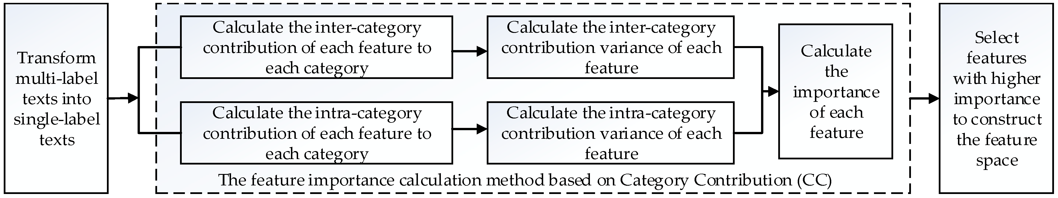
3. Proposed Method

In this paper, a feature importance calculation method based on CC is proposed, and based on this method, a feature selection method for multi-label text is proposed. The process of the feature selection method proposed in this paper is shown in Figure 1.

The purpose of feature selection is to select features with strong category discrimination ability. Calculating the importance of each feature accurately and selecting features with higher importance to construct the feature space are very important for the classification performance. In this paper, the contribution of features to the classification is considered from two aspects of inter-category and intra-category, and a method of feature importance based on CC is proposed. The main steps of the feature importance method are as follows.

(1)

The inter-category contribution and intra-category contribution of each feature to each category are calculated respectively.

(2)

For each feature, the inter-category contribution variance and intra-category contribution variance are calculated respectively based on the inter-category contribution and intra-category contribution to each category calculated in (1).

(3)

The importance of each feature is calculated by fusing the intra-category contribution variance and the inter-category contribution variance.

3.1. Category Contribution

Category contribution refers to the role that the features play in distinguishing one category from others, including inter-category contribution and intra-category contribution.

3.1.1. Inter-Category Contribution

If a feature appears many times in category a, while rarely appears in other categories, thus, the feature may be closely associated with category a and contributes a lot to distinguish category a. Therefore, we calculate the contribution of a feature to the classification based on the number of samples with the feature in one category and the average number of samples with the feature in other categories. In this method, the contribution is calculated by the occurrence of the feature among different categories, so we call it inter-category contribution.

The information entropy measures the uncertainty between random variables in a quantified form [37]. In text processing, information entropy can be used to describe the distribution of features in different categories. The distribution of the feature in different categories reflects the contribution of the feature to the classification. Therefore, we introduce the information entropy of the feature into the calculation of inter-category contribution in this paper. The information entropy of the feature F_j is as follows.

$$H(F_j)=-{\displaystyle \sum _{k=1}^q\frac{T_f(F_j,L_k)}{T_F(F_j)}\log }\frac{T_f(F_j,L_k)}{T_F(F_j)}$$

(11)

where T_F (F_j) is the number of samples with F_j in the training set, T_f (F_j,L_k) is the number of samples with F_j in category k, and q is the number of categories.

The more uniformly the feature is distributed in different categories, the greater the information entropy of the feature is, and vice versa. Therefore, the formula for calculating the inter-category contribution of the feature F_j based on information entropy is as follows.

$$e_{jk}=\sqrt{{(T_f(F_j,L_k)-\frac{{\displaystyle {\sum }_{t=1}^q{T}_f(F_j,L_t)-T_f(F_j,L_k)}}{q-1})}^2}\lg (\frac{1}{H(F_j)+0.0001}+1)$$

(12)

where e_jk is the inter-category contribution of F_j to category k, T_f (F_j,L_k) is the number of samples with F_j in category k, H(F_j) is the information entropy of F_j and q is the number of categories.

3.1.2. Intra-Category Contribution

If a feature appears in one sample in category a, but appears in all samples in category b, thus, the feature may be a word occasionally appearing in category a, but a very relevant word to category b. Therefore, we calculate the contribution of the feature to the classification by the proportion of the number of samples with the feature in the category to the total number of samples in the category. The proportion reflects the degree of correlation between the feature and the category. In this method, the contribution is calculated by the occurrence of the feature in one category, so we call it intra-category contribution.

$$r_{jk}=\frac{T_f(F_j,L_k)}{N_k}$$

(13)

where r_jk is the intra-category contribution of F_j to category k, T_f (F_j,L_k) is the number of samples with F_j in category k, and N_k is the total number of samples in category k.

The intra-category contribution of the feature is a value between 0 and 1, including 0 and 1. The closer the value is to 1, the greater the contribution of the feature to the classification of the category is.

3.2. Feature Importance Calculation Method Based on Category Contribution

Calculating the importance of each feature accurately and selecting features with higher importance to construct the feature space directly determine the performance of classification. In this paper, the contribution of the feature to classification is considered from two aspects of inter-category and intra-category, and a method of feature importance based on CC is proposed.

Let E_j={e_1j,e_2j,…,e_qj} denote the inter-category contribution set of the feature F_j in q categories, and R_j={r_1j,r_2j,…,r_qj} denote the intra-category contribution set of the feature F_j in q categories. When the difference between the data in E_j is great, the category discrimination ability of F_j is strong and when the difference between the data in R_j is great, the category discrimination ability of F_j is strong too. In this paper, the variance is used to represent the difference between the data in the set. The variance of the data in E_j and R_j are called the inter-category contribution variance and intra-category contribution variance respectively. The formulas are as follows.

$$V_E(F_j)=\frac{{\displaystyle \sum (e_{jk}-\overline{e_j}}{)}^2}{q}$$

(14)

$$V_R(F_j)=\frac{{\displaystyle \sum (r_{jk}-\overline{r_j}}{)}^2}{q}$$

(15)

where V_E(F_j) is the inter-category contribution variance of F_j, V_R(F_j) is the intra-category contribution variance of F_j, e_jk is the inter-category contribution of F_j to category k, r_jk is the intra-category contribution of F_j to category k, $\overline{e_j}$ is the mean inter-category contribution of F_j, ${\overline{r}}_j$ is the mean intra-category contribution of F_j and q is the number of categories.

The greater the inter-category contribution variance and intra-category contribution variance are, the stronger the category discrimination ability of the feature is. Therefore, it is necessary to consider from the perspective of making the inter-category contribution variance and intra-category contribution variance both greater when defining the formula of feature importance calculation. In the field of information retrieval, F-measure is the harmonic mean of precision and recall, which ensures that both precision and recall get a greater value [38]. Based on this idea, the formula for feature importance calculation is defined as follows.

$$f(F_j)=\frac{2\ast V_E\left(F_j\right)\ast V_R\left(F_j\right)}{V_E\left(F_j\right)+V_R\left(F_j\right)}$$

(16)

where f (F_j) is the feature importance of F_j.

After the importance of each feature is calculated, the features with higher importance are selected based on the predefined dimension, to construct the feature space.

4. Experiment and Results

4.1. Data Sets

In order to demonstrate the effectiveness of the proposed method, we collected six public multi-label text data sets, including the fields of medical, business, computers, entertainment, health, and social [39,40], from the Mulan website (http://mulan.sourceforge.net/datasets.html) for experiments.

For the data set S, we describe it from five aspects: the number of samples |S|, the number of features dim(S), the number of categories L(S), label cardinality LCard(S), and label density LDen(S). The data set S is defined as follows.

$$S=\{(x_i,Y_i)|1\le i\le p\}$$

(17)

where x_i is a sample, Y_i is the set of categories of x_i and p is the number of samples in S.

Label cardinality, which measures the average number of categories per sample.

$$LCard(S)=\frac{1}{p}{\displaystyle {\sum }_{i=1}^p\left|Y_i\right|}$$

(18)

Label density, which is the label cardinality normalized by the number of categories.

$$LDen(S)=\frac{1}{L(S)}\ast LCard(S)$$

(19)

Details of the experimental data sets are described in

Table 1. Data sets description.

NO.	Data set	|S|	dim(S)	L(S)	LCard(S)	LDen(S)
1	Medical	978	1449	45	1.2454	0.0277
2	Business	11,214	438	30	1.5990	0.0533
3	Computers	12,444	681	33	1.5072	0.0457
4	Entertainment	12,730	640	21	1.4137	0.0673
5	Health	9205	612	32	1.6441	0.0514
6	Social	12,111	1047	39	1.2793	0.0328

.

4.2. Evaluation Metrics

The results of the multi-label classification experiments were evaluated by the following five evaluation metrics, which are described in FormulaS (20)–(24) [41].

In order to describe these formulas conveniently, we define the following variables: $S=\{(x_i,Y_i)|1\le i\le p\}$ denotes a multi-label test set, $\gamma =\{L_1,L_2,\cdots ,L_q\}$ denotes the category set, $h(x_i)$ denotes the multi-label classifier, $f(x_i,L_s)$ denotes the prediction function and ${rank}_f(x_i,L_s)$ denotes the ranking function. Where x_i is a sample, Y_i is the set of categories of x_i, and $Y_i\subseteq \gamma$, and p is the number of samples in S. Also, if $f(x_i,L_s)>f(x_i,L_t)$, then ${rank}_f(x_i,L_s)<{rank}_f(x_i,L_t)$.

Average precision (AP), which evaluates the average fraction of categories ranked above a particular category L_s. The higher the value is, the better the performance is.

$$AP=\frac{1}{p}{\displaystyle \sum _{i=1}^p\frac{1}{\left|Y_i\right|}}{\displaystyle \sum _{L\in Y_i}\frac{\left|\right\{L_s|{rank}_f(x_i,L_s)\le {rank}_f(x_i,L),L_s\in Yi\}|}{{rank}_f(x_i,L)}}$$

(20)

Hamming loss (HL), which evaluates how many times a sample-label pair is misclassified. The smaller the value is, the better the performance is.

$$HL=\frac{1}{p}{\displaystyle \sum _{i=1}^p\frac{1}{q}}|h(x_i)\Delta Y_i|$$

(21)

where $\Delta$ denotes the symmetric difference between two sets.

One error (OE), which evaluates how many times the top-ranked category is not in the set of proper categories of the sample. The smaller the value is, the better the performance is.

$$OE=\frac{1}{p}{\displaystyle \sum _{i=1}^p\left[\arg \underset{L\in \gamma }{\max }f(x_i,L)\notin Y_i\right]}$$

(22)

where for any predicate π, [π] equals 1 if π holds and 0 otherwise.

Coverage (CV), which evaluates how many steps are needed, on average, to move down the category list in order to cover all the proper categories of the sample. The smaller the value is, the better the performance is.

$$CV=\frac{1}{p}{\displaystyle \sum _{i=1}^p\underset{L\in Y_i}{\max }}{rank}_f(x_i,L)-1$$

(23)

Ranking loss (RL), which evaluates the average fraction of category pairs that are not correctly ordered. The smaller the value is, the better the performance is.

$$RL=\frac{1}{p}{\displaystyle \sum _{i=1}^p\frac{1}{\left|Y_i\right|\left|\overline{Y_i}\right|}}|(L_s,L_t)|f(x_i,L_s)\le f(x_i,L_t),(L_s,L_t)\in Y_i\ast \overline{Y_i}\}|$$

(24)

where $\overline{Y_i}$ denotes the complementary set of $Y_i$ in $\gamma$.

4.3. Experimental Settings

In order to demonstrate the effectiveness of the proposed method, we designed two parts of experiments.

(1) Proposed algorithm validation experiment. This part includes two groups of experiments. In the first group, in different feature space dimensions, the proposed feature selection method is compared with the baseline method which keeps all features to demonstrate the effectiveness of the proposed method. ALA is used to transform multi-label texts into single-label texts, and BRKNN and MLKNN are used as the classifiers. For MLKNN, the number of nearest neighbors and the value of smooth are set as 10 and 1 respectively [42]. For BRKNN, the number of hidden neurons is set as 20% of the number of features in the feature space, the learning rate is set as 0.05, and the number of iterations for training is set as 100 [42]. Let t denote the proportion of the dimension of the feature space to the dimension of the original feature space, this is, t denotes the proportion of the number of selected features to the number of all features. We run experiments of this group with the value of t ranging from 10% to 90%, and 10% as an interval. In the second group, the method based on CC proposed in the paper is performed on different label assignment methods to further demonstrate the effectiveness of the proposed method. BRKNN is used as the classifier and the value of t ranges from 10% to 50%, with 10% as an interval.

(2) Performance comparison experiment. In this part, we compare the performance of the proposed feature selection method with that of the commonly used feature selection methods to demonstrate the effectiveness of the proposed method. The feature selection method based on DF and the feature selection method based on MI are selected as the comparison methods. ALA is used to transform multi-label texts into single-label texts, and BRKNN is used as the classifier. The value of t ranges from 10% to 50%, with 10% as an interval.

All the code in this paper is implemented in MyEclipse version 2014 in a Windows 10 using 3.30 GHz Intel (R) CPU with 8 GB of RAM. The Term Frequency-Inverse Document Frequency (TF-IDF) method [43] is used to calculate the weight of the feature in each text. BRKNN and MLKNN multi-label classification algorithms are implemented based on MULAN software package [44]. The cross validation is used in the experiments. And all the experimental results shown in this paper are the average of ten-fold cross validation.

4.4. Experimental Results and Analysis

4.4.1. Proposed Algorithm Validation Experiment

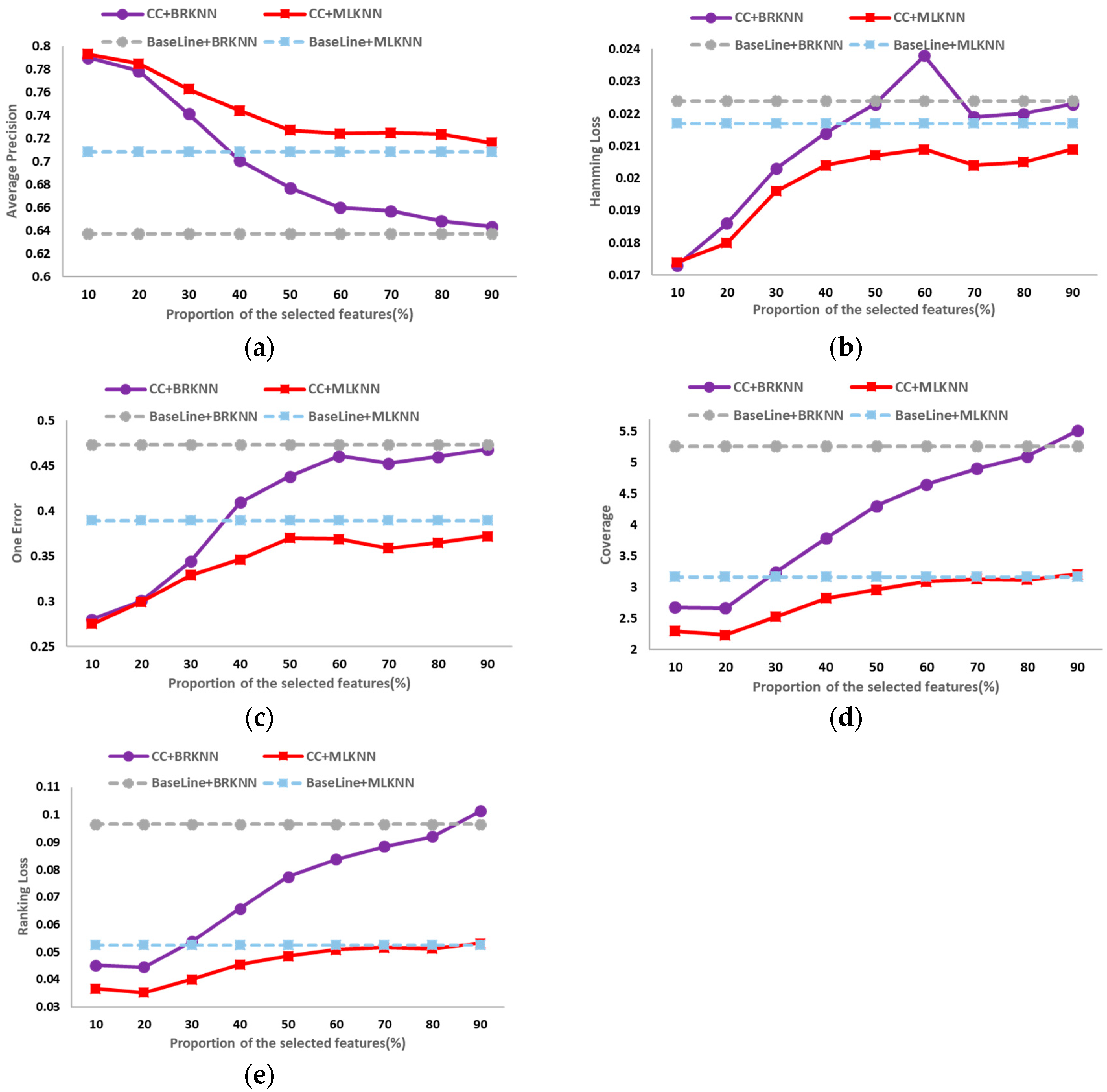
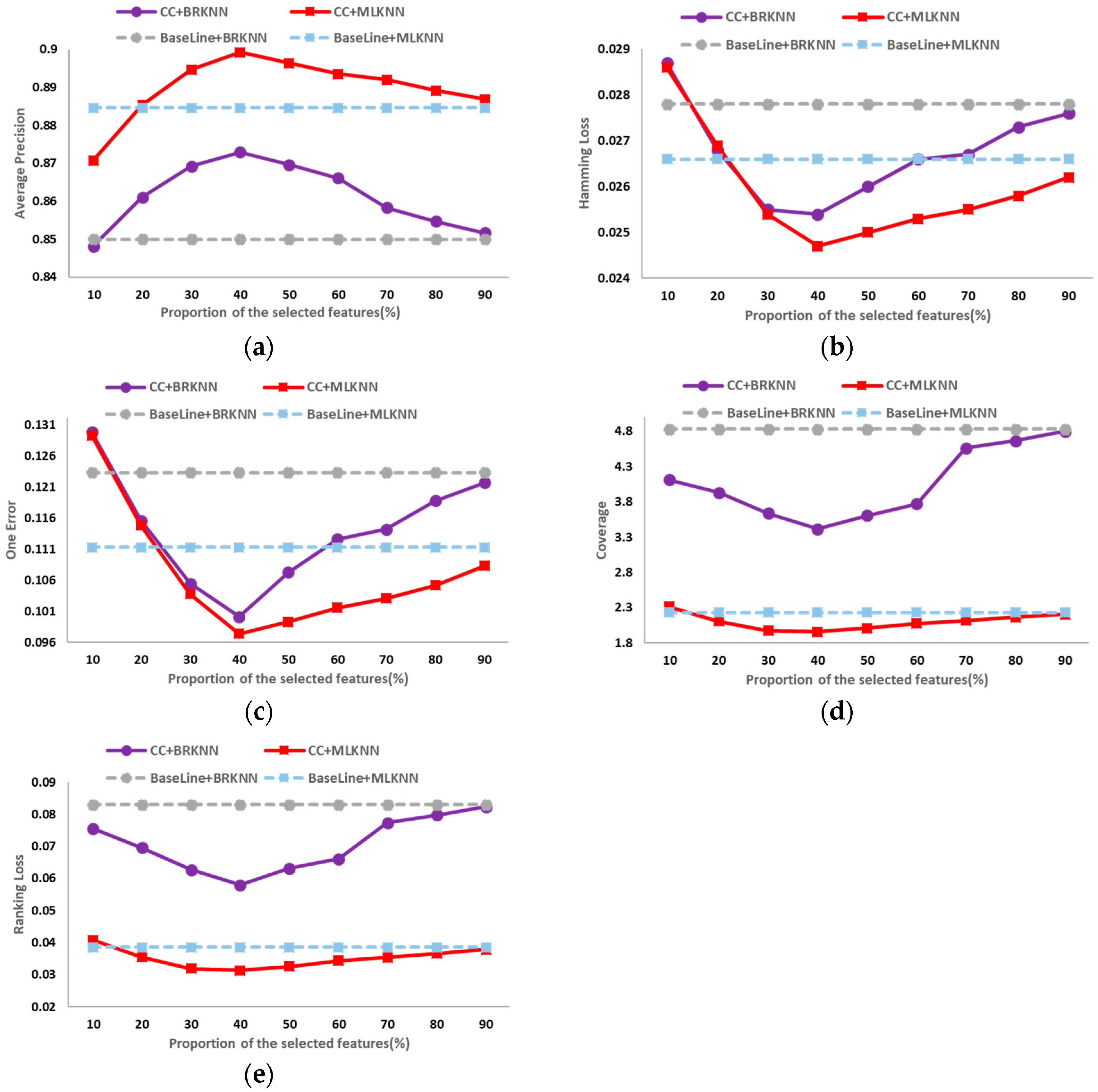
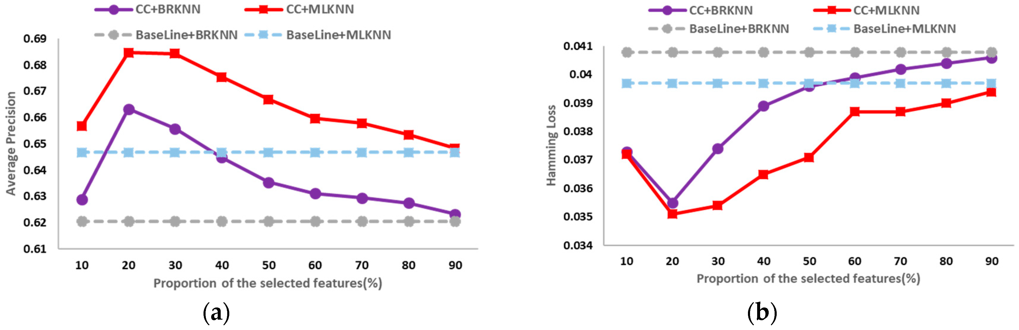
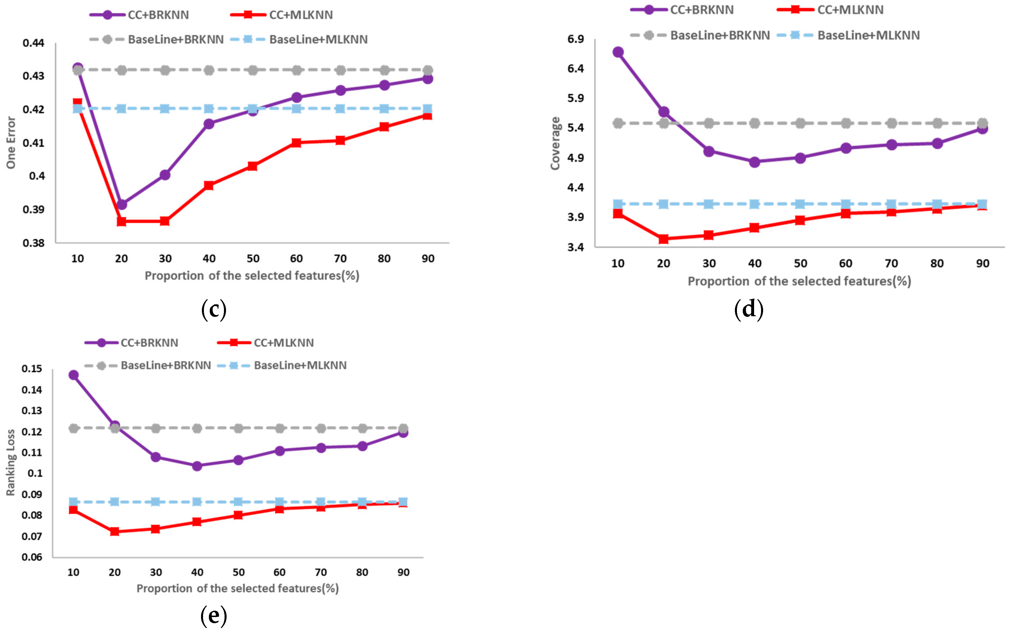
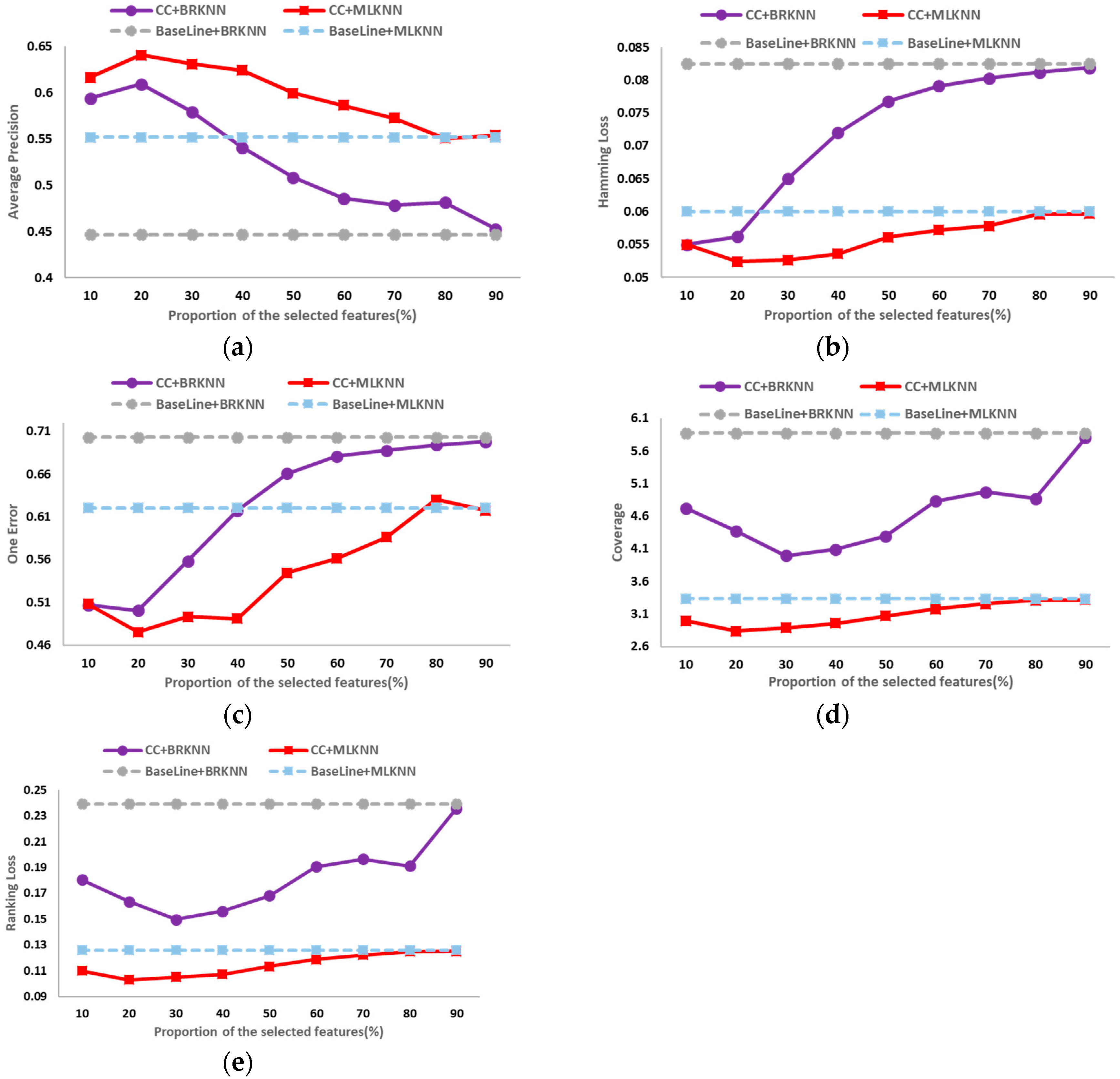
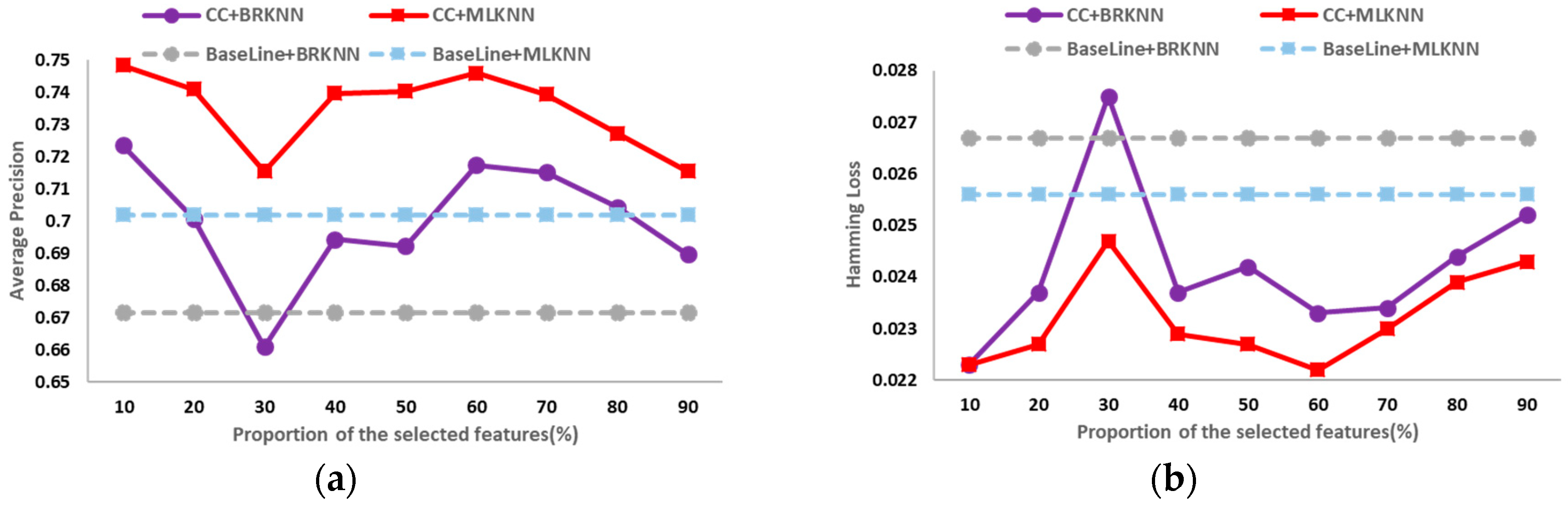
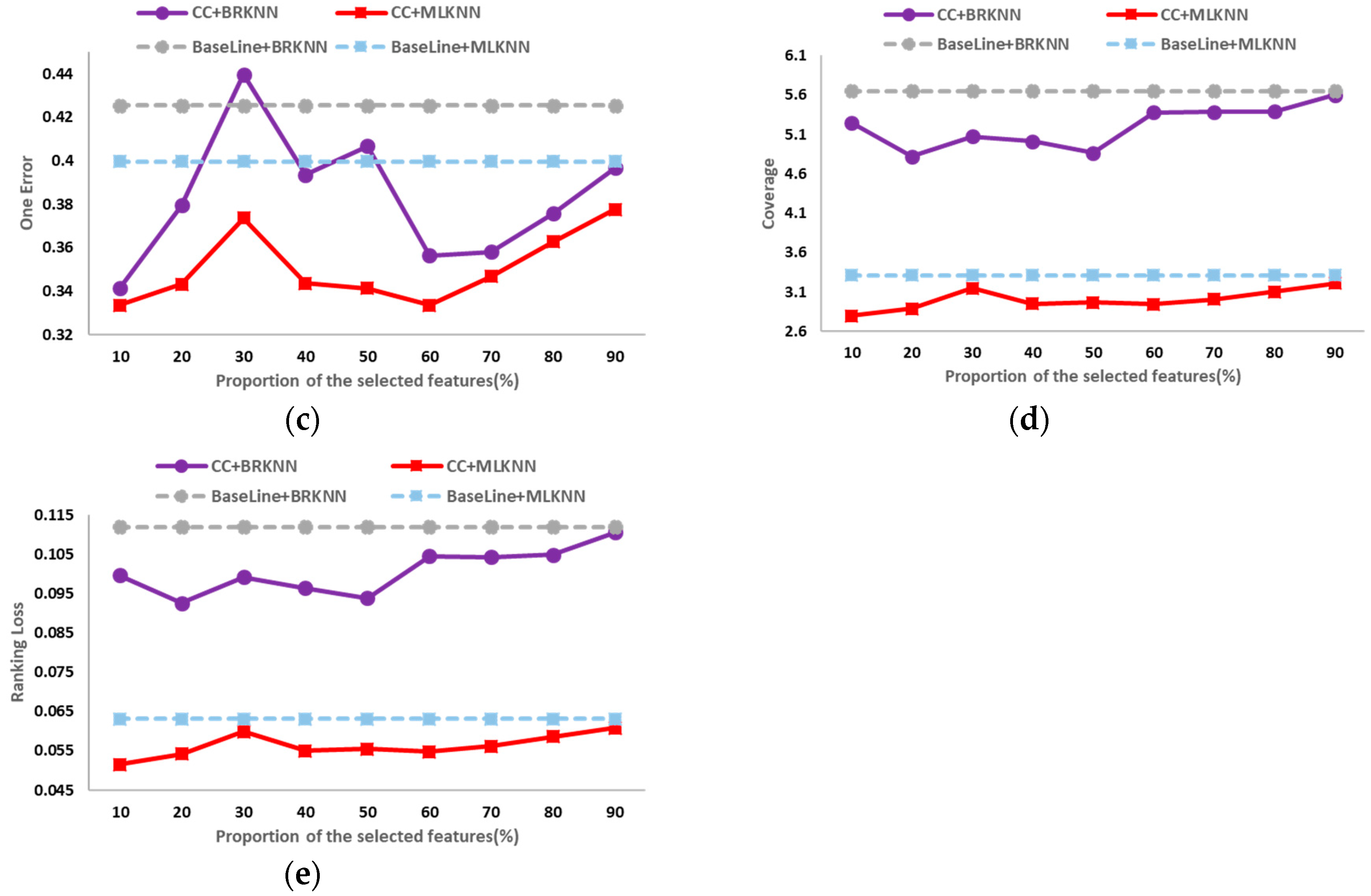
The classification results on the six public data sets in different dimensions of average precision, hamming loss, one error, coverage and ranking loss are shown in Figure 2, Figure 3, Figure 4, Figure 5, Figure 6 and Figure 7. In these figures, the horizontal axis denotes the proportion of the selected features, that is, the horizontal axis denotes the value of t, and the vertical axis denotes the value of the evaluation metric; CC+BRKNN denotes that the multi-label classification is performed on the feature space constructed by the proposed method, and BRKNN is used as the classifier; CC+MLKNN denotes that the multi-label classification is performed on the feature space constructed by the proposed method, and MLKNN is used as the classifier; BaseLine+BRKNN denotes that the multi-label classification is performed on the original feature space, and BRKNN is used as the classifier; and BaseLine+MLKNN denotes that the multi-label classification is performed on the original feature space, and MLKNN is used as the classifier.

It can be seen from Figure 2 to Figure 7 that, on the six data sets, the classifications performed on the feature spaces constructed by the proposed feature selection method universally have better performance than that of the baseline method in each dimension. In classification experiments, the average precision is the most intuitive and concerned evaluation metric. Therefore, we regard the best value of the average precision as the best performance of the classification, so as to analyze the experimental results. Compared with the classification results in the original feature space, the increase (decrease) percentage of each evaluation metric is shown in

Table 2. Increase (decrease) percentage of each evaluation metrics on six data sets.

Data Set	Algorithm	t	AP(%)↑	HL(%)↓	OE(%)↓	CV(%)↓	RL(%)↓
Medical	BRKNN	10%	23.92	22.77	40.81	49.16	53.21
	MLKNN	10%	11.91	19.82	29.39	27.52	30.10
Business	BRKNN	40%	2.69	8.63	18.82	29.29	30.20
	MLKNN	40%	1.65	7.14	12.49	12.29	18.91
Computers	BRKNN	20%	6.88	12.99	9.33	-3.59*	-1.07*
	MLKNN	20%	5.88	11.59	8.07	14.17	16.42
Entertainment	BRKNN	20%	36.39	31.88	28.82	25.56	31.58
	MLKNN	20%	16.09	12.67	23.39	14.88	18.25
Health	BRKNN	20%	67.79	54.09	44.32	38.30	43.77
	MLKNN	30%	9.96	22.47	20.99	15.38	21.59
Social	BRKNN	10%	7.74	16.48	19.76	7.03	10.98
	MLKNN	10%	6.61	12.89	16.56	15.62	18.35

.

From Table 2, it can be seen that on the six data sets, most of the classification evaluation metrics obtained in the feature space constructed by the proposed method are universally better than those obtained in the original feature space. Only on the Computers data set, when the value of t is 20% and BRKNN is used as the classifier, the coverage and ranking loss obtained in the feature space constructed by the proposed method are worse than those obtained in the original feature space. Excitingly, on the Health data set, when the value of t is 20% and BRKNN is used as the classifier, the average precision is increased by 67.79%, which is the greatest increase among all.

In order to further demonstrate the effectiveness of the proposed feature importance method based on CC, we experimented it on ALA, NLA, LLA, and SLA.

The experimental results of the six public data sets are shown in

Table 3. Experimental results on Medical data set.

Algorithm	Evaluation	BaseLine	10%	20%	30%	40%	50%	Average
ALA	AP	0.6375	0.7900	0.7786	0.7413	0.7010	0.6770	0.7376
	HL	0.0224	0.0173	0.0186	0.0203	0.0214	0.0223	0.0200
	OE	0.4734	0.2802	0.3007	0.3446	0.4099	0.4386	0.3548
	CV	5.2680	2.6780	2.6681	3.2413	3.7864	4.3058	3.3359
	RL	0.0966	0.0452	0.0446	0.0538	0.0658	0.0775	0.0574
NLA	AP	0.4264	0.6053	0.4808	0.4587	0.4424	0.4346	0.4844
	HL	0.0277	0.0224	0.0262	0.0268	0.0272	0.0274	0.0260
	OE	0.6769	0.4929	0.6248	0.6452	0.6626	0.6697	0.6190
	CV	8.5582	5.3865	7.2309	7.8667	8.1998	8.3575	7.4083
	RL	0.1724	0.1003	0.1422	0.1566	0.1642	0.1678	0.1462
LLA	AP	0.6431	0.7939	0.7736	0.7403	0.7093	0.6847	0.7404
	HL	0.0229	0.0164	0.0196	0.0206	0.0221	0.0234	0.0204
	OE	0.4673	0.2761	0.3098	0.3548	0.4038	0.4355	0.3560
	CV	5.1517	3.0082	2.8911	3.2850	3.6169	3.9974	3.3597
	RL	0.0942	0.0487	0.0475	0.0550	0.0633	0.0709	0.0571
SLA	AP	0.6431	0.7977	0.7786	0.7423	0.7015	0.6764	0.7393
	HL	0.0229	0.0166	0.0188	0.0205	0.0223	0.0232	0.0203
	OE	0.4673	0.2638	0.3048	0.3549	0.4120	0.4477	0.3566
	CV	5.1517	2.6885	2.5881	3.1583	3.8354	4.1709	3.2882
	RL	0.0942	0.0454	0.0432	0.0523	0.0672	0.0751	0.0566

,

Table 4. Experimental results on Business data set.

Algorithm	Evaluation	BaseLine	10%	20%	30%	40%	50%	Average
ALA	AP	0.8500	0.8482	0.8611	0.8692	0.8729	0.8696	0.8642
	HL	0.0278	0.0287	0.0268	0.0255	0.0254	0.0260	0.0265
	OE	0.1233	0.1298	0.1156	0.1055	0.1001	0.1073	0.1117
	CV	4.8337	4.1161	3.9341	3.6375	3.4179	3.6064	3.7424
	RL	0.0831	0.0756	0.0696	0.0627	0.0580	0.0632	0.0658
NLA	AP	0.8617	0.8668	0.8713	0.8696	0.8684	0.8662	0.8685
	HL	0.0413	0.0259	0.0252	0.0310	0.0353	0.0378	0.0310
	OE	0.1323	0.1328	0.1277	0.1279	0.1271	0.1283	0.1288
	CV	2.6461	2.5978	2.5058	2.5241	2.5443	2.5792	2.5502
	RL	0.0510	0.0492	0.0462	0.0468	0.0475	0.0487	0.0477
LLA	AP	0.8459	0.8518	0.8626	0.8685	0.8644	0.8585	0.8612
	HL	0.0283	0.0289	0.0269	0.0260	0.0260	0.0267	0.0269
	OE	0.1286	0.1315	0.1177	0.1104	0.1083	0.1144	0.1165
	CV	4.9435	3.9726	3.8237	3.4919	4.0517	4.2886	3.9257
	RL	0.0853	0.0731	0.0672	0.0596	0.0691	0.0734	0.0685
SLA	AP	0.8459	0.8460	0.8648	0.8697	0.8687	0.8650	0.8628
	HL	0.0283	0.0287	0.0267	0.0256	0.0260	0.0266	0.0267
	OE	0.1286	0.1305	0.1141	0.1077	0.1071	0.1128	0.1144
	CV	4.9435	4.2223	3.7887	3.5617	3.4172	3.6875	3.7355
	RL	0.0853	0.0784	0.0664	0.0612	0.0587	0.0651	0.0660

,

Table 5. Experimental results on Computers data set.

Algorithm	Evaluation	BaseLine	10%	20%	30%	40%	50%	Average
ALA	AP	0.6206	0.6290	0.6633	0.6558	0.6448	0.6354	0.6457
	HL	0.0408	0.0373	0.0355	0.0374	0.0389	0.0396	0.0377
	OE	0.4319	0.4327	0.3916	0.4005	0.4159	0.4197	0.4121
	CV	5.4837	6.6824	5.6804	5.0189	4.8361	4.9038	5.4243
	RL	0.1218	0.1472	0.1231	0.1080	0.1039	0.1066	0.1178
NLA	AP	0.6106	0.6357	0.6468	0.6306	0.6185	0.6134	0.6290
	HL	0.0421	0.0380	0.0386	0.0405	0.0413	0.0417	0.0400
	OE	0.4449	0.4211	0.4081	0.4265	0.4368	0.4427	0.4270
	CV	5.2835	5.5427	5.0874	5.0331	5.1437	5.1691	5.1952
	RL	0.1199	0.1286	0.1142	0.1124	0.1155	0.1163	0.1174
LLA	AP	0.6202	0.6308	0.6527	0.6503	0.6393	0.6344	0.6415
	HL	0.0408	0.0371	0.0366	0.0381	0.0394	0.0401	0.0383
	OE	0.4341	0.4226	0.4024	0.4099	0.4196	0.4262	0.4161
	CV	5.4456	6.7910	5.8355	5.1061	4.9505	4.9109	5.5188
	RL	0.1204	0.1508	0.1261	0.1082	0.1069	0.1067	0.1197
SLA	AP	0.6202	0.6322	0.6659	0.6576	0.6405	0.6345	0.6461
	HL	0.0408	0.0372	0.0354	0.0373	0.0390	0.0395	0.0377
	OE	0.4341	0.4301	0.3905	0.4012	0.4151	0.4219	0.4118
	CV	5.4456	6.5895	5.5776	5.0150	5.0003	4.9911	5.4347
	RL	0.1204	0.1453	0.1206	0.1081	0.1090	0.1089	0.1184

,

Table 6. Experimental results on Entertainment data set.

Algorithm	Evaluation	BaseLine	10%	20%	30%	40%	50%	Average
ALA	AP	0.4468	0.5939	0.6094	0.5797	0.5408	0.5084	0.5664
	HL	0.0825	0.0550	0.0562	0.0650	0.0720	0.0768	0.0650
	OE	0.7031	0.5068	0.5005	0.5585	0.6177	0.6607	0.5688
	CV	5.8738	4.7235	4.3727	3.9918	4.0888	4.2952	4.2944
	RL	0.2394	0.1804	0.1638	0.1499	0.1561	0.1681	0.1637
NLA	AP	0.4487	0.6285	0.6279	0.5593	0.5039	0.4775	0.5594
	HL	0.0856	0.0587	0.0608	0.0707	0.0781	0.0816	0.0700
	OE	0.7047	0.4820	0.4806	0.5629	0.6335	0.6673	0.5653
	CV	4.2258	3.9436	3.7231	3.8558	4.0325	4.1280	3.9366
	RL	0.1687	0.1553	0.1438	0.1502	0.1591	0.1638	0.1544
LLA	AP	0.4448	0.5814	0.6000	0.5779	0.5311	0.5123	0.5605
	HL	0.0829	0.0569	0.0546	0.0658	0.0738	0.0780	0.0658
	OE	0.7049	0.5264	0.5112	0.5533	0.6316	0.6647	0.5774
	CV	5.9031	4.8710	4.4250	4.1108	4.0846	4.3590	4.3701
	RL	0.2407	0.1860	0.1653	0.1535	0.1553	0.1673	0.1655
SLA	AP	0.4448	0.5914	0.6100	0.5786	0.5335	0.5087	0.5644
	HL	0.0829	0.0554	0.0565	0.0659	0.0737	0.0778	0.0659
	OE	0.7049	0.5133	0.4936	0.5588	0.6303	0.6682	0.5728
	CV	5.9031	4.7438	4.3654	4.0314	4.1107	4.2302	4.2963
	RL	0.2407	0.1812	0.1631	0.1501	0.1574	0.1646	0.1633

,

Table 7. Experimental results on Health data set.

Algorithm	Evaluation	BaseLine	10%	20%	30%	40%	50%	Average
ALA	AP	0.3977	0.6490	0.6673	0.6288	0.4893	0.4527	0.5774
	HL	0.0893	0.0434	0.0410	0.0418	0.0482	0.0824	0.0514
	OE	0.7045	0.4311	0.3923	0.4598	0.6324	0.6667	0.5165
	CV	9.1015	6.1071	5.6158	5.0217	5.1979	5.8342	5.5553
	RL	0.1981	0.1227	0.1114	0.1004	0.1106	0.1257	0.1142
NLA	AP	0.4868	0.6743	0.6294	0.5599	0.5164	0.5015	0.5763
	HL	0.0657	0.0450	0.0504	0.0584	0.0628	0.0643	0.0562
	OE	0.7300	0.4115	0.4890	0.6118	0.6837	0.7083	0.5809
	CV	4.3185	4.2340	4.1030	4.1283	4.2314	4.2801	4.1954
	RL	0.0922	0.0893	0.0851	0.0861	0.0894	0.0910	0.0882
LLA	AP	0.3986	0.6479	0.6639	0.5821	0.5018	0.4612	0.5714
	HL	0.0893	0.0431	0.0417	0.0434	0.0570	0.0785	0.0527
	OE	0.7047	0.4295	0.3987	0.5340	0.6084	0.6633	0.5268
	CV	9.0197	6.0337	5.6436	5.3229	5.6505	5.6923	5.6686
	RL	0.1962	0.1207	0.1111	0.1061	0.1164	0.1200	0.1149
SLA	AP	0.3986	0.6496	0.6680	0.5571	0.4717	0.4545	0.5602
	HL	0.0893	0.0433	0.0410	0.0435	0.0497	0.0815	0.0518
	OE	0.7047	0.4306	0.3892	0.5662	0.6544	0.6656	0.5412
	CV	9.0197	6.0943	5.6392	5.2713	5.6608	5.8244	5.6980
	RL	0.1962	0.1223	0.1122	0.1085	0.1227	0.1256	0.1183

and

Table 8. Experimental results on Social data set.

Algorithm	Evaluation	BaseLine	10%	20%	30%	40%	50%	Average
ALA	AP	0.6716	0.7236	0.7008	0.6610	0.6944	0.6923	0.6944
	HL	0.0267	0.0223	0.0237	0.0275	0.0237	0.0242	0.0243
	OE	0.4255	0.3414	0.3796	0.4398	0.3937	0.4068	0.3923
	CV	5.6477	5.2504	4.8211	5.0733	5.0137	4.8636	5.0044
	RL	0.1120	0.0997	0.0926	0.0993	0.0965	0.0939	0.0964
NLA	AP	0.6083	0.6711	0.6504	0.6231	0.6125	0.6117	0.6338
	HL	0.0315	0.0267	0.0279	0.0301	0.0311	0.0313	0.0294
	OE	0.5214	0.4270	0.4580	0.4983	0.5161	0.5170	0.4833
	CV	4.5495	4.7592	4.4514	4.4851	4.5952	4.5599	4.5702
	RL	0.0933	0.0987	0.0907	0.0916	0.0945	0.0935	0.0938
LLA	AP	0.6684	0.7089	0.6912	0.5948	0.7012	0.6986	0.6789
	HL	0.0264	0.0231	0.0251	0.0283	0.0234	0.0237	0.0247
	OE	0.4308	0.3563	0.3908	0.5909	0.3768	0.3806	0.4191
	CV	5.6894	5.6646	5.2306	5.3454	5.7251	5.7900	5.5511
	RL	0.1127	0.1095	0.1007	0.1060	0.1127	0.1134	0.1085
SLA	AP	0.6685	0.7154	0.6977	0.6583	0.6892	0.6955	0.6912
	HL	0.0264	0.0230	0.0245	0.0268	0.0241	0.0241	0.0245
	OE	0.4308	0.3535	0.3858	0.4448	0.4017	0.3887	0.3949
	CV	5.6838	5.4147	4.8384	5.1892	5.0926	5.7444	5.2559
	RL	0.1126	0.1032	0.0931	0.1024	0.0983	0.1131	0.1020

. In these tables, BaseLine denotes the multi-label classifications performed on the original feature space; 10%, 20%, 30%, 40%, and 50% denote the multi-label classifications performed on the feature spaces in different dimensions, respectively; and Average denotes the average of the classification results in five different dimensions.

From Table 3 to Table 8, it can be seen that the feature importance method based on CC performed on ALA, NLA, LLA, and SLA all can effectively select the features with strong category discrimination ability. The performance of the classifications based on the feature space constructed by the proposed method is all superior to that on the original feature space, demonstrating that the proposed feature importance method is effective and universal.

4.4.2. Performance Comparison Experiment

In this section, we demonstrate the effectiveness of the proposed method by comparing its performance with that of the feature selection method based on DF and the feature selection method based on MI. The classification results on the six data sets in different dimensions using different feature selection methods are shown in

Table 9. Comparison of classification performance on Medical data set.

Evaluation	Algorithm	10%	20%	30%	40%	50%
AP↑	CC+BRKNN	0.7900	0.7786	0.7413	0.7010	0.6770
	DF+BRKNN	0.7357	0.7577	0.7438	0.7175	0.6821
	MI+BRKNN	0.4122	0.3979	0.3776	0.3521	0.3368
HL↓	CC+BRKNN	0.0173	0.0186	0.0203	0.0214	0.0223
	DF+BRKNN	0.0198	0.0199	0.0200	0.0207	0.0210
	MI+BRKNN	0.0274	0.0275	0.0275	0.0273	0.0275
OE↓	CC+BRKNN	0.2802	0.3007	0.3446	0.4099	0.4386
	DF+BRKNN	0.3395	0.3252	0.3395	0.3793	0.4191
	MI+BRKNN	0.7086	0.7516	0.8221	0.7976	0.8078
CV↓	CC+BRKNN	2.6780	2.6681	3.2413	3.7864	4.3058
	DF+BRKNN	3.8861	3.0769	3.4942	3.8064	4.7442
	MI+BRKNN	7.2564	7.3207	7.3809	8.5993	8.6850
RL↓	CC+BRKNN	0.0452	0.0446	0.0538	0.0658	0.0775
	DF+BRKNN	0.0693	0.0499	0.0586	0.0660	0.0851
	MI+BRKNN	0.1372	0.1381	0.1398	0.1706	0.1732

,

Table 10. Comparison of classification performance on Business data set.

Evaluation	Algorithm	10%	20%	30%	40%	50%
AP↑	CC+BRKNN	0.8482	0.8611	0.8692	0.8729	0.8696
	DF+BRKNN	0.8460	0.8541	0.8567	0.8606	0.8561
	MI+BRKNN	0.8330	0.8362	0.8424	0.8453	0.8433
HL↓	CC+BRKNN	0.0287	0.0268	0.0255	0.0254	0.0260
	DF+BRKNN	0.0283	0.0276	0.0275	0.0266	0.0273
	MI+BRKNN	0.0293	0.0289	0.0288	0.0285	0.0284
OE↓	CC+BRKNN	0.1298	0.1156	0.1055	0.1001	0.1073
	DF+BRKNN	0.1309	0.1253	0.1218	0.1130	0.1188
	MI+BRKNN	0.1342	0.1317	0.1314	0.1309	0.1308
CV↓	CC+BRKNN	4.1161	3.9341	3.6375	3.4179	3.6064
	DF+BRKNN	4.2224	3.9910	3.9218	4.1443	4.3527
	MI+BRKNN	4.7304	4.6595	4.1774	3.9514	4.3903
RL↓	CC+BRKNN	0.0756	0.0696	0.0627	0.0580	0.0632
	DF+BRKNN	0.0781	0.0719	0.0700	0.0718	0.0755
	MI+BRKNN	0.0912	0.0882	0.0782	0.0719	0.0810

,

Table 11. Comparison of classification performance on Computers data set.

Evaluation	Algorithm	10%	20%	30%	40%	50%
AP↑	CC+BRKNN	0.6290	0.6633	0.6558	0.6448	0.6354
	DF+BRKNN	0.6352	0.6532	0.6480	0.6391	0.6314
	MI+BRKNN	0.5900	0.6093	0.6148	0.6135	0.6171
HL↓	CC+BRKNN	0.0373	0.0355	0.0374	0.0389	0.0396
	DF+BRKNN	0.0360	0.0363	0.0382	0.0395	0.0399
	MI+BRKNN	0.0407	0.0401	0.0409	0.0416	0.0415
OE↓	CC+BRKNN	0.4327	0.3916	0.4005	0.4159	0.4197
	DF+BRKNN	0.4149	0.3991	0.4093	0.4203	0.4253
	MI+BRKNN	0.4699	0.4491	0.4446	0.4483	0.4435
CV↓	CC+BRKNN	6.6824	5.6804	5.0189	4.8361	4.9038
	DF+BRKNN	6.7307	5.7193	5.0377	4.8693	4.9880
	MI+BRKNN	7.5324	6.5456	5.8639	5.5300	5.4504
RL↓	CC+BRKNN	0.1472	0.1231	0.1080	0.1039	0.1066
	DF+BRKNN	0.1476	0.1230	0.1080	0.1042	0.1081
	MI+BRKNN	0.1682	0.1454	0.1283	0.1204	0.1184

,

Table 12. Comparison of classification performance on Entertainment data set.

Evaluation	Algorithm	10%	20%	30%	40%	50%
AP↑	CC+BRKNN	0.5939	0.6094	0.5797	0.5408	0.5084
	DF+BRKNN	0.5631	0.5611	0.5219	0.5070	0.4894
	MI+BRKNN	0.4702	0.4764	0.4687	0.4544	0.4409
HL↓	CC+BRKNN	0.0550	0.0562	0.0650	0.0720	0.0768
	DF+BRKNN	0.0574	0.0631	0.0724	0.0768	0.0789
	MI+BRKNN	0.0648	0.0714	0.0803	0.0844	0.0867
OE↓	CC+BRKNN	0.5068	0.5005	0.5585	0.6177	0.6607
	DF+BRKNN	0.5482	0.5628	0.6287	0.6580	0.6742
	MI+BRKNN	0.6799	0.6914	0.7279	0.7443	0.7555
CV↓	CC+BRKNN	4.7235	4.3727	3.9918	4.0888	4.2952
	DF+BRKNN	5.1703	4.6991	4.4675	4.4405	4.7396
	MI+BRKNN	5.7741	5.2273	4.6481	4.5380	4.6361
RL↓	CC+BRKNN	0.1804	0.1638	0.1499	0.1561	0.1681
	DF+BRKNN	0.2004	0.1787	0.1723	0.1730	0.1884
	MI+BRKNN	0.2312	0.2082	0.1857	0.1803	0.1837

,

Table 13. Comparison of classification performance on Health data set.

Evaluation	Algorithm	10%	20%	30%	40%	50%
AP↑	CC+BRKNN	0.6490	0.6673	0.6288	0.4893	0.4527
	DF+BRKNN	0.6668	0.6669	0.4925	0.4645	0.4424
	MI+BRKNN	0.5605	0.5774	0.5420	0.4385	0.4195
HL↓	CC+BRKNN	0.0434	0.0410	0.0418	0.0482	0.0824
	DF+BRKNN	0.0411	0.0416	0.0524	0.0807	0.0842
	MI+BRKNN	0.0503	0.0499	0.0499	0.0507	0.0816
OE↓	CC+BRKNN	0.4311	0.3923	0.4598	0.6324	0.6667
	DF+BRKNN	0.3986	0.3897	0.6242	0.6435	0.6684
	MI+BRKNN	0.5345	0.5145	0.5808	0.6853	0.7023
CV↓	CC+BRKNN	6.1071	5.6158	5.0217	5.1979	5.8342
	DF+BRKNN	6.0885	5.5838	5.8472	6.9259	7.4004
	MI+BRKNN	7.5864	6.7204	5.9721	6.1377	6.0252
RL↓	CC+BRKNN	0.1227	0.1114	0.1004	0.1106	0.1257
	DF+BRKNN	0.1208	0.1107	0.1239	0.1467	0.1586
	MI+BRKNN	0.1638	0.1432	0.1276	0.1352	0.1331

and

Table 14. Comparison of classification performance on Social data set.

Evaluation	Algorithm	10%	20%	30%	40%	50%
AP↑	CC+BRKNN	0.7236	0.7008	0.6610	0.6944	0.6923
	DF+BRKNN	0.7081	0.6724	0.6097	0.6863	0.6912
	MI+BRKNN	0.5817	0.5924	0.5906	0.5421	0.6016
HL↓	CC+BRKNN	0.0223	0.0237	0.0275	0.0237	0.0242
	DF+BRKNN	0.0226	0.0271	0.0276	0.0238	0.0232
	MI+BRKNN	0.0310	0.0312	0.0313	0.0321	0.0308
OE↓	CC+BRKNN	0.3414	0.3796	0.4398	0.3937	0.4068
	DF+BRKNN	0.3525	0.4203	0.5522	0.4043	0.3916
	MI+BRKNN	0.5355	0.5464	0.5385	0.6141	0.5044
CV↓	CC+BRKNN	5.2504	4.8211	5.0733	5.0137	4.8636
	DF+BRKNN	5.8012	4.9990	5.8213	5.4352	5.9549
	MI+BRKNN	7.4690	6.2813	6.4551	8.1137	8.3188
RL↓	CC+BRKNN	0.0997	0.0926	0.0993	0.0965	0.0939
	DF+BRKNN	0.1118	0.0969	0.1154	0.1063	0.1180
	MI+BRKNN	0.1549	0.1286	0.1287	0.1675	0.1732

.

In these tables, CC denotes the proposed feature selection method, DF denotes the feature selection method based on DF, MI denotes the feature selection method based on MI, CC+BRKNN denotes the multi-label classification performed on the feature space constructed by the proposed method, and BRKNN is used as the classifier. The naming rules for other symbols are the same. Also, we use bold font to denote the best performance in one dimension and underline to denote the best performance in all dimensions.

From Table 9 to Table 14, it can be seen that there are 150 comparison results using three feature selection algorithms on six data sets with five evaluation metrics. Among them, the feature selection method based on CC wins 126 times, and the winning percentage is up to 84.0%.

Aside from dimensions, the five evaluation metrics have 30 best values on six data sets, 29 of which are obtained in the feature selection method based on CC proposed in this paper. In addition, in the proposed feature selection method, most of the best values of the evaluation metrics are obtained when the dimensions are 10% and 20%, only a few are obtained when the dimension are 30% and 40%, but none when the dimension is 50%.

From the perspective of the average precision, compared with the method base on DF, the evaluation metric has the largest increase on the Entertainment data set, which is 8.22%, and compared with the method based on MI, the evaluation metric has the largest increase on the Medical data set, which is 91.65%.

Therefore, the performance of the multi-label text feature selection method based on CC is better than that of the common feature selection methods based on DF and MI. Also, the best values of the evaluation metrics are all obtained in smaller dimensions, which greatly reduces the feature space dimension and improves the classification performance.

In summary, it can be seen from the experimental results and analysis on the six data sets that

(1)

Compared with the baseline method, the classification performance of the feature selection method proposed in this paper are generally superior in all dimensions, which demonstrates the effectiveness of the proposed method.

(2)

Good classification performance has been achieved when the proposed method of feature importance is performed on different label assignment methods, demonstrating that the feature importance method based on CC is effective and universal.

(3)

Compared with the commonly used feature selection methods, the percentage of the best values of the evaluation metrics obtained on the proposed feature selection method is 84.0%, demonstrating that the proposed method has a good performance.

(4)

The best values of the evaluation metrics are obtained in the proposed multi-label feature selection method all in smaller dimensions, which has an obvious dimension reduction effect, and is suitable for high-dimensional text data.

5. Conclusions

Aiming at the high dimensionality and sparsity of text feature space, a multi-label text feature selection method was proposed in this paper. Firstly, the label assignment method was used to transformed multi-label texts into single-label texts. Then, on this basis, an importance method based on CC was proposed to calculate the importance of each feature. Finally, features with higher importance were selected to construct the feature space. In the proposed method, the multi-label feature selection problem has been transformed into a single-label one. Thus, the feature selection process is simple and fast, and the dimension reduction effect is obvious. The proposed method is very suitable for high-dimensional text data. Compared with the baseline method and the commonly used feature selection methods, the proposed feature selection methods all achieved better performance on the six public data sets, which demonstrates the effectiveness of the method.

In this paper, a method of feature importance based on CC is proposed from the perspective of category. The contribution of features to classification of different categories was calculated from two aspects of inter-category and intra-category, clarifying the importance of features to different categories, and selecting features with strong category classification ability. The proposed method has a good performance.

However, the proposed algorithm does not consider the correlation between categories, which should be studied in the future.