Peridynamic Modeling of Mode-I Delamination Growth in Double Cantilever Composite Beam Test: A Two-Dimensional Modeling Using Revised Energy-Based Failure Criteria

Abstract

This study presents a two-dimensional ordinary state-based peridynamic (OSB PD) modeling of mode-I delamination growth in a double cantilever composite beam (DCB) test using revised energy-based failure criteria. The two-dimensional OSB PD composite model for DCB modeling is obtained by reformulating the previous OSB PD lamina model in x–z direction. The revised energy-based failure criteria are derived following the approach of establishing the relationship between critical bond breakage work and energy release rate. Loading increment convergence analysis and grid spacing influence study are conducted to investigate the reliability of the present modeling. The peridynamic (PD) modeling load–displacement curve and delamination growth process are then quantitatively compared with experimental results obtained from standard tests of composite DCB samples, which show good agreement between the modeling results and experimental results. The PD modeling delamination growth process damage contours are also illustrated. Finally, the influence of the revised energy-based failure criteria is investigated. The results show that the revised energy-based failure criteria improve the accuracy of the PD delamination modeling of DCB test significantly.

1. Introduction

Carbon fiber-reinforced polymer (CFRP) composite materials have been widely used in aerospace structures due to their high specific stiffness/strength, low coefficient of thermal expansion, and excellent fatigue resistance. In the design procedure of composite structures, testing and analysis are both needed due to the overall consideration of cost and reliability. Laminate delamination is one of the main failure modes of composite structures and, hence, has become a major concern of CFRP composite design and analysis for many years [1,2,3,4,5]. Currently, the most widely used analysis method for capturing delamination initiation and growth of CFRP composites is based on the framework of finite element method (FEM), such as cohesive zone element (CZE) and virtual crack closure technique (VCCT). Although these techniques have been successfully applied to many delamination problems of CFRP composites [6,7,8], they usually have to preset the delamination growth path, which is difficult for many real engineering problems. Besides, as stated in [9,10,11,12], these conventional analysis methods based on classical continuum mechanics require that the displacement field of body be continuously differential in space. This requirement is in contradiction with inherent spatial discontinuity existing in delamination growth problems.

As an alternative to conventional analysis method, Silling et al. [13,14,15] introduced the peridynamic (PD) theory of solid mechanics, which attempts to unite the mathematical modeling of continuous media, cracks, and particles within a single framework. Peridynamic theory replaces the partial differential equation of the classical theory of solid mechanics with integral or integral-differential equations, and “spontaneous” formation of fracture and damage of composites could be simulated without any prior knowledge of damage path [16,17,18,19]. Peridynamic theory has been successfully applied to capture the delamination damage of CFRP composites. The interlayer delamination damage patterns of composite laminate under low velocity impact were given by Askari et al. [11] and Xu et al. [10]. The delamination damages between each layer of composite laminates with notch or open hole were presented by Hu et al. [20,21,22,23]. “Spontaneous” delamination damages were captured by peridynamic theory in these works, without any presetting of delamination path or refinement of the delamination front mesh.

Although the above works have proved the potential advantages of peridynamic theory in delamination modeling of CFRP composites, currently, few studies have focused on the quantitative delamination growth modeling of CFRP composite by peridynamics. Double cantilever composite beam (DCB) test provides a good benchmark example for validating an approach’s basic ability in modeling mode-I delamination in composites. It is meaningful to conduct DCB modeling work to examine the reliability of an approach in modeling structural delamination problem, such as for CZE [24,25] and VCCT [26]. Hu et al. [12] developed an energy-based approach to simulate delamination in composites using bond-based peridynamics. Delamination growth in double cantilever beam (DCB) test is simulated and the convex delamination front was well captured.

In the present study, a two-dimensional ordinary state-based peridynamic (OSB PD) modeling of mode-I delamination growth of CFRP composite DCB test is presented. Double cantilever beam (DCB) test is the basic experiment to measure mode-I delamination fracture toughness, G_IC, of CFRP composites. This simple loading case provides a good benchmark example to quantitatively verify the ability of peridynamic theory in modeling delamination growth of CFRP composites. The two-dimensional OSB PD composite model used in the present study for DCB modeling is obtained by reformulating the previous OSB PD lamina model [27] in the x–z direction. The revised energy-based failure criteria are derived following the approach proposed by Silling et al. [15] of establishing the relationship between critical bond breakage work and energy release rate. Loading increment convergence analysis and grid spacing influence study are conducted. Comparisons of load–displacement curve and delamination growth process between PD modeling results and experimental results are shown. Delamination growth process damage contours are illustrated. Numerical results using revised and original energy-based failure criteria are also compared.

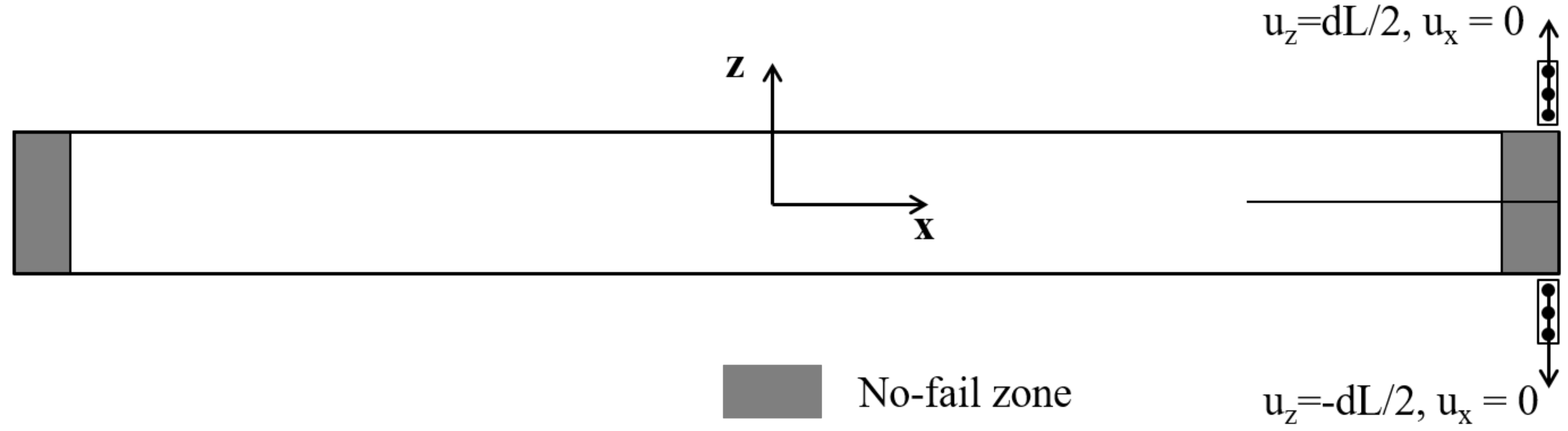
2. Two-Dimensional Ordinary State-Based Peridynamic Model for DCB Modeling

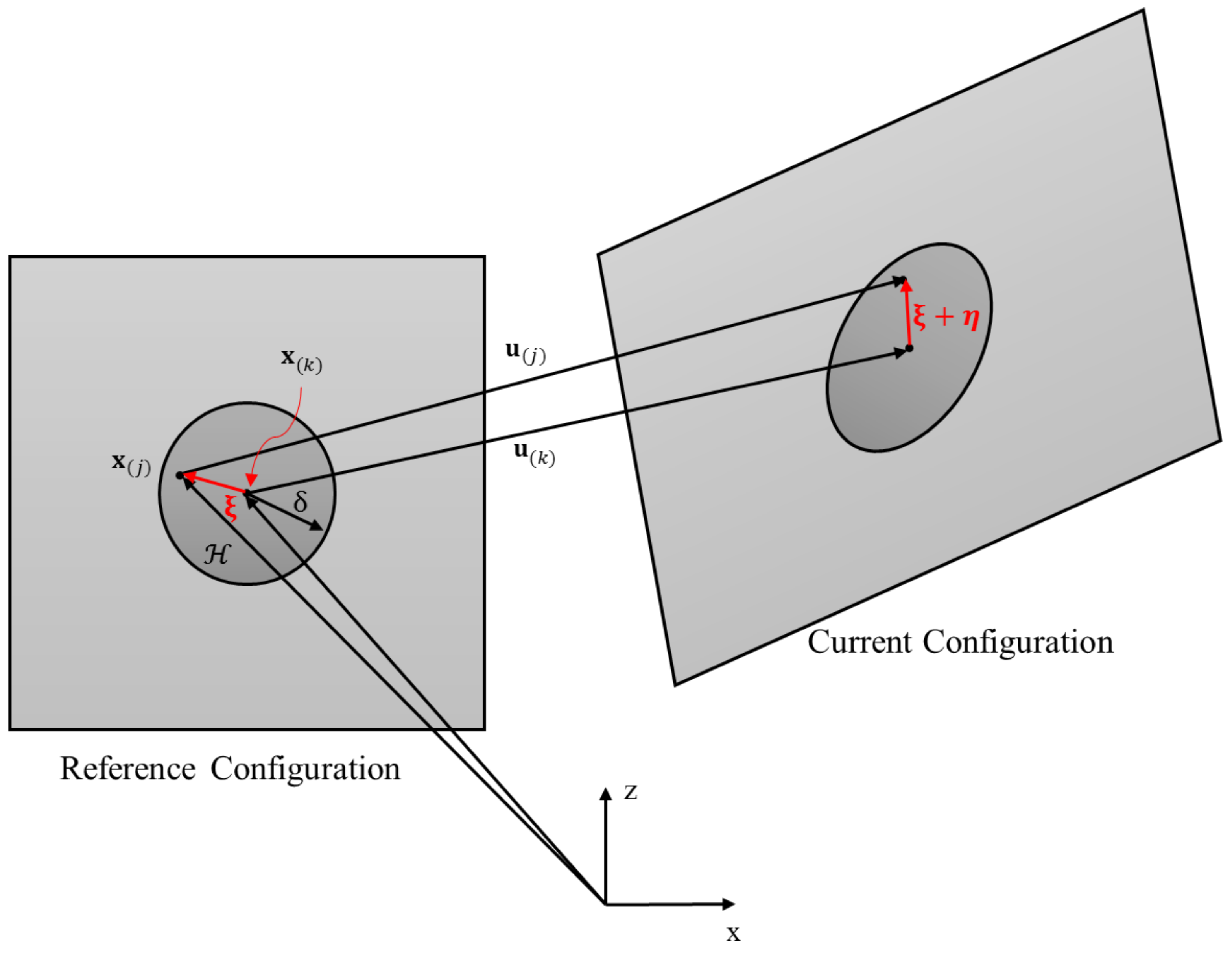
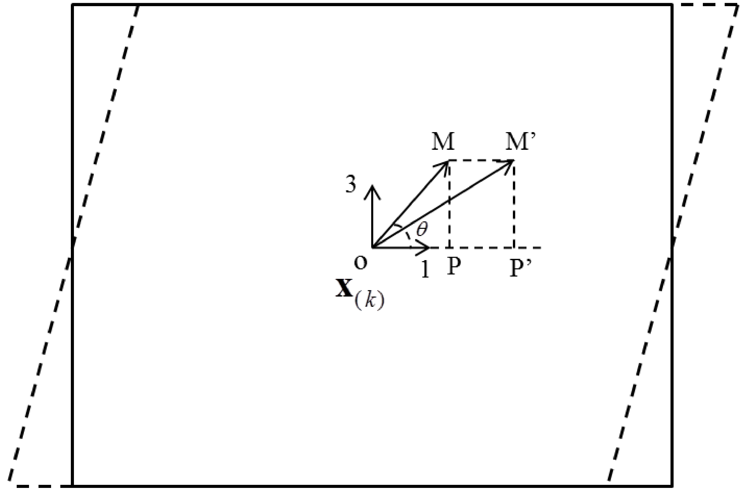
2.1. Governing Equation

The two-dimensional OSB PD composite model used in the present study for DCB modeling is obtained by reformulating the previous OSB PD lamina model (Madenci and Oterkus [27]) in x–z direction. The detailed derivation process is given in Appendix A. The governing equation of the present two-dimensional OSB PD composite model can be written as

$${\rho }_{(k)}{\mathbf{ü}}_{(k)}={\displaystyle \sum _{j=1}^{\infty }[t_{(k)(j)}}-t_{(j)(k)}]V_{(j)}+b_{(k)},$$

(1)

where ${\rho }_{(k)}$ is the density of material point $x_{(k)}$, $\stackrel{}{{\mathbf{ü}}_{(k)}}$ is instantaneous acceleration of $x_{(k)}$, as shown in Figure 1, $b_{(k)}$ is the external load density, and $t_{(k)(j)}$ and $t_{(j)(k)}$ are PD force density between $x_{(k)}$ and $x_{(j)}$. The PD force density can be expressed as

$$t_{(k)(j)}=A_{(k)(j)}\frac{y_{(j)}-y_{(k)}}{\left|y_{(j)}-y_{(k)}\right|},$$

(2)

$$t_{(j)(k)}=B_{(j)(k)}\frac{y_{(k)}-y_{(j)}}{\left|y_{(k)}-y_{(j)}\right|},$$

(3)

with

$$A_{(k)(j)}=2ad\frac{\delta }{\left|x_{(j)}-x_{(k)}\right|}{\Lambda }_{(k)(j)}{\theta }_{(k)}+2\delta b{s}_{(k)(j)}+2\delta ({\mu }_F{b}_F+{\mu }_Z{b}_Z)s_{(k)(j)},$$

(4)

$$B_{(j)(k)}=2ad\frac{\delta }{\left|x_{(k)}-x_{(j)}\right|}{\Lambda }_{(j)(k)}{\theta }_{(j)}+2\delta b{s}_{(j)(k)}+2\delta ({\mu }_F{b}_F+{\mu }_Z{b}_Z)s_{(j)(k)},$$

(5)

and

$$s_{(k)(j)}=\frac{\left|y_{(j)}-y_{(k)}\right|-\left|x_{(j)}-x_{(k)}\right|}{\left|x_{(j)}-x_{(k)}\right|},$$

(6)

and

$${\mu }_F=\{\begin{array}{c}1\\ 0\end{array}\begin{array}{c} (x_{(j)}-x_{(k)})\parallel \mathrm{fiber} \mathrm{direction}\\ \mathrm{otherwise}\end{array},$$

(7)

$${\mu }_Z=\{\begin{array}{c}1\\ 0\end{array}\begin{array}{c} (x_{(j)}-x_{(k)})\perp \mathrm{fiber} \mathrm{direction}\\ \mathrm{otherwise}\end{array},$$

(8)

where $s_{(k)(j)}$ is the stretch of bonds, and $\delta$ is the radius of the horizon zone. The direction cosines of the relative position vectors between the material points $x_{(k)}$ and $x_{(j)}$ in the undeformed and deformed states are defined as

$${\Lambda }_{(k)(j)}=\frac{y_{(j)}-y_{(k)}}{\left|y_{(j)}-y_{(k)}\right|}\cdot \frac{x_{(j)}-x_{(k)}}{\left|x_{(j)}-x_{(k)}\right|}.$$

(9)

The PD dilatation ${\theta }_{(k)}$ can be expressed as

$${\theta }_{(k)}=d{\displaystyle \sum _{j=1}^{\infty }\delta s_{(k)(j)}{\Lambda }_{(k)(j)}{V}_{(j)}}.$$

(10)

The PD material parameters a, d characterize the effect of dilatation, and b, b_F, b_Z are associated with deformation of material points in arbitrary directions, fiber direction, and thickness direction, respectively. These parameters are related to material properties of CFRP composite and horizon radius. The detailed derivation procedures to get these PD material parameters are illustrated in Appendix A.2. These PD material parameters are related to composite material parameters as

$$a=\frac{1}{2}(Q_{13}-Q_{55}),$$

(11)

$$d=\frac{2}{\pi {\delta }^3},$$

(12)

$$b=\frac{6Q_{55}}{\pi {\delta }^4},$$

(13)

$$b_F=\frac{Q_{11}-Q_{13}-2Q_{55}}{2\delta {\displaystyle \sum _{j=1}^J\left|x_{(j)}-x_{(k)}\right|V_{(j)}}},$$

(14)

$$b_Z=\frac{Q_{33}-Q_{13}-2Q_{55}}{2\delta {\displaystyle \sum _{j=1}^J\left|x_{(j)}-x_{(k)}\right|V_{(j)}}},$$

(15)

where $Q_{11}$, $Q_{33}$, $Q_{13}$, and $Q_{55}$ are coefficients of stiffness matrix $\left[Q\right]$ presented in Appendix A.1.

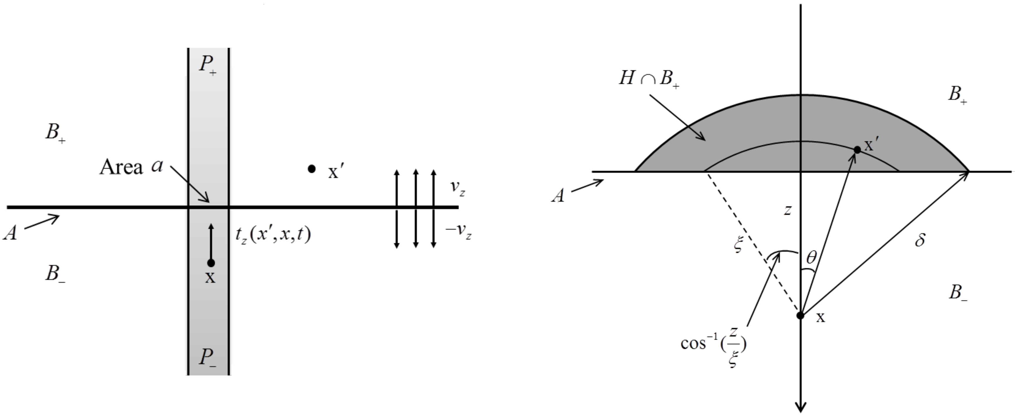
2.2. Revised Energy-Based Failure Criteria

Following the approach for deriving the relationship between critical bond breakage work and energy release rate by Silling et al. [15], revised two-dimensional energy-based failure criteria for mode-I delamination growth of CFRP composites are proposed. The influence of the revised energy-based failure criteria will be investigated in Section 4.3.

This approach assumes that the energy consumed by a growing delamination front equals the work required, per unit delamination front area, to separate two halves of a body across a plane (Figure 2). Suppose a plane $A$ separates two halves of a two-dimensional body $B$ into $B_{+}$ and $B_{-}$. The delamination front area $a$ is on the plane. Consider a mode-I delamination motion with velocity field on Figure 2. The total energy $E$ absorbed by $P$ in this motion is

$$E={\displaystyle {\int }_0^t{W}_{abs}(P)d{t}^{\prime }={\displaystyle {\int }_0^{t_0}{\displaystyle {\int }_P{\displaystyle {\int }_B{t}_z(v_z{}^{\prime }-v_z)d{V}^{\prime }dVdt}}}}.$$

(16)

The assumed critical bond breakage work $w_{\mathrm{IC}}$ in this motion is

$${\displaystyle {\int }_0^{t_0}{t}_z(v_z{}^{\prime }-v_z)dt}=w_{\mathrm{IC}}.$$

(17)

Therefore,

$$\begin{array}{ll}E & =w_{\mathrm{IC}}{\int }_P{\int }_{B}d{V}^{\prime }dV=w_{\mathrm{IC}}({\int }_{P_{-}}{\int }_{B_{+}\backslash P_{+}}d{V}^{\prime }dV+{\int }_{P_{+}}{\int }_{B_{-}\backslash P_{-}}d{V}^{\prime }dV+{\int }_{P_{-}}{\int }_{P_{+}}d{V}^{\prime }dV)\\ & =w_{\mathrm{IC}}(2{\int }_{P_{-}}{\int }_{B_{+}}d{V}^{\prime }dV-{\int }_{P_{-}}{\int }_{P_{+}}d{V}^{\prime }dV)\\ & =w_{\mathrm{IC}}(2a{\int }_0^{\delta }{\int }_z^{\delta }{\int }_{{-\cos }^{-1}(z/\xi )}^{{\cos }^{-1}(z/\xi )}\xi d\theta d\xi dz-a{\int }_0^{\delta }a(\delta -z)dz)\\ & =w_{\mathrm{IC}}(\frac{4}{3}a{\delta }^3-\frac{1}{2}{a}^2{\delta }^2)\end{array},$$

(18)

For Equation (18), as stated by Silling et al. [15], bonds that do not cross plane $A$ have no contributions to the integrand. However, in the present study, bonds that cross plane $A$ are separated into three parts: bonds connecting $P_{-}$ and $B_{+}\backslash P_{+}$, bonds connecting $P_{+}$ and $B_{-}\backslash P_{-}$, and bonds connecting $P_{-}$ and $P_{+}$, as shown in Figure 2. The bond breakage work between $P_{-}$ and $P_{+}$ is calculated only once compared with the original procedure in [15]. Adding these three parts of the bond breakage work together gives the revised total absorbed energy $E$ shown in Equation (18).

Assuming this total absorbed energy equals the critical energy release rate times the area of delamination front,

$$G_{\mathrm{IC}}=E/a=w_{\mathrm{IC}}(\frac{4}{3}{\delta }^3-\frac{1}{2}a{\delta }^2).$$

(19)

Thus, the critical bond breakage work for mode-I delamination is related to critical energy release rate,

$$w_{\mathrm{IC}}=\frac{G_{\mathrm{IC}}}{\frac{4}{3}{\delta }^3-\frac{1}{2}a{\delta }^2}.$$

(20)

For two-dimensional numerical modeling, the delamination front area $a$ can be set as the discretized grid spacing $dx$,

$$w_{\mathrm{IC}}=\frac{G_{\mathrm{IC}}}{\frac{4}{3}{\delta }^3-\frac{1}{2}dx{\delta }^2}.$$

(21)

From the above derivation, revised energy-based failure criteria for mode-I delamination growth are proposed as

$$\left|\frac{w_{\mathrm{I}}}{w_{\mathrm{IC}}}\right|\ge 1, w_{\mathrm{IC}}=\frac{G_{\mathrm{IC}}}{\frac{4}{3}{\delta }^3-\frac{1}{2}dx{\delta }^2}, w_{\mathrm{I}}={\displaystyle {\int }_0^t{t}_z(v_z{}^{\prime }-v_z)dt}=t_z(w^{\prime }-w).$$

(22)

Local damage at a material point is defined as the weighted ratio of the number of eliminated interactions to the total number of initial interactions of the material point with its family members [28].

The status variable for delamination damage, $\mu$, is defined as

$$\mu =\{\begin{array}{l}1, \left|\frac{w_{\mathrm{I}}}{w_{\mathrm{IC}}}\right| <1 \mathrm{no} \mathrm{damage}\hfill \\ 0, \left|\frac{w_{\mathrm{I}}}{w_{\mathrm{IC}}}\right| \ge 1 \mathrm{damage} \hfill \end{array}.$$

(23)

The delamination damage between ply (n) and (n + 1) at a point can be quantified as

$$\{\begin{array}{l}{\phi }_{\mathrm{out}-\mathrm{of}-\mathrm{plane}\_\mathrm{upper}}^{(n)}=1-\frac{{\displaystyle \sum _{j=1}^{N_{(k)}^{(\mathrm{upper})}}{\mu }_{(k)(j)}^{(n)(m)}}}{N_{(k)}^{(\mathrm{upper})}}\hfill \\ {\phi }_{\mathrm{out}-\mathrm{of}-\mathrm{plane}\_\mathrm{lower}}^{(n+1)}=1-\frac{{\displaystyle \sum _{j=1}^{N_{(k)}^{(\mathrm{lower})}}{\mu }_{(k)(j)}^{(n)(m)}}}{N_{(k)}^{(\mathrm{lower})}}\hfill \\ {\phi }_{\mathrm{delamination}}^{(n)(n+1)}=\frac{1}{2}({\phi }_{\mathrm{out}-\mathrm{of}-\mathrm{plane}\_\mathrm{upper}}^{(n)}+{\phi }_{\mathrm{out}-\mathrm{of}-\mathrm{plane}\_\mathrm{lower}}^{(n+1)}).\hfill \end{array}$$

(24)

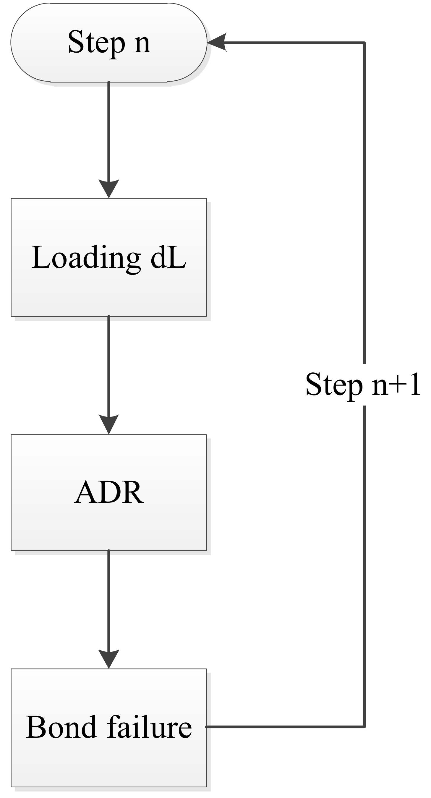
2.3. Numerical Implementation

Although the peridynamic governing equation is in dynamic form, it can still be used to solve quasi-static or static problems [29,30,31]. Adaptive dynamic relaxation (ADR) method [29] is currently the most widely used method to solve quasi-static or static problems for PD. ADR method is particularly effective for solving highly nonlinear problems, including geometric and material nonlinearities [31].

According to the ADR method, Equation (1) at the n^th iteration can be rewritten as

$${\ddot{U}}^n(X,t^n)+c^n{\dot{U}}^n(X,t^n)=D^{-1}{F}^n(U^n,{U^{\prime }}^n,X,X^{\prime }),$$

(25)

where $D$ is the fictitious diagonal density matrix and $c$ is the damping coefficient which can be expressed by

$$c^n=2\sqrt{({(U^n)}^T{}^1\mathbf{K}{}^n{U}^n)/({(U^n)}^T{U}^n)},$$

(26)

in which ${}^1\mathbf{K}{}^n$ is the diagonal “local” stiffness matrix, which is given as

$${}^{1}K{}_{{}^{ii}}^n=-(F_i^n/{\lambda }_{ii}-F_i^{n-1}/{\lambda }_{ii})/(\Delta t{\dot{u}}_i^{n-1/2}),$$

(27)

where $F_i^n$ is the value of force vector $F^n$ at material point $x$, which includes both the peridynamic force state vector and external forces, and ${\lambda }_{ii}$ are the diagonal elements of $D$ which should be large enough to avoid numerical divergence.

By utilizing central-difference explicit integration, displacements and velocities for the next time step can be obtained:

$${\dot{U}}^{n+1/2}=\frac{((2-c^n\Delta t){\dot{U}}^{n-1/2}+2\Delta t{D}^{-1}{F}^n)}{(2+c^n\Delta t)}$$

(28)

and

$${\dot{U}}^{n+1}=U^n+\Delta t{\dot{U}}^{n+1/2}.$$

(29)

To start the iteration process, we assume that $U^0\ne 0$ and ${\dot{U}}^0=0$, so the integration can be started by

$${\dot{U}}^{1/2}=\frac{\Delta t{D}^{-1}{F}^0}{2}.$$

(30)

Due to the large computational amount of PD model, GPU-parallel computing is introduced. The PGI CUDA FORTRAN compiler, PGI/17.10 Community Edition, is used for compiling. The GPU node at Cranfield University Delta HPC Cluster is applied for running the GPU-parallel program. The GPU block threads are fixed to 256, and the number of blocks depend on the total number of parallel processes [32].

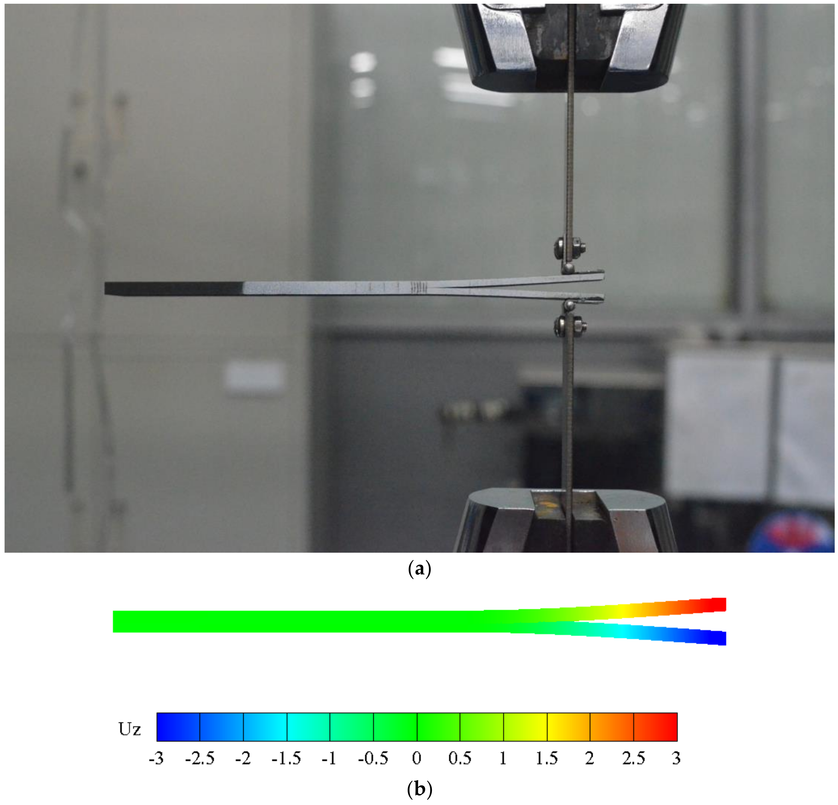
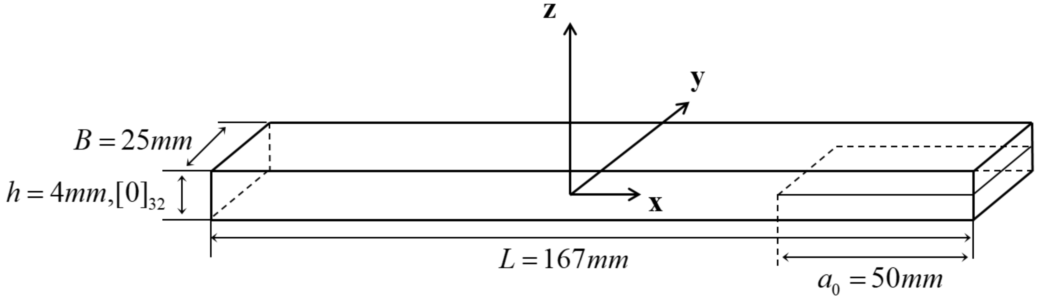
3. Experimental Setup and Results

In order to validate the reliability of the present two-dimensional OSB PD composite model, a CFRP double cantilever beam (DCB) test is conducted. The CFRP composite DCB test setup is shown in Figure 3a. The experiment was conducted in accordance with ASTM standard D5528-13 [33]. The DCB test specimens are bonded with two piano hinges at the initial delamination end. White paint marking is sprayed on the side of the specimen for visualizing the delamination front position. As shown in Figure 4, the length of the specimen is 167 mm, with 25 mm width and 4 mm thickness. The layup of the specimen is [0]₃₂, with 0.125 mm/ply. Initial delamination $a_0=50 \mathrm{mm}$ is preset on the mid-plane of the specimen, between Layer 16 and 17. In this experiment, five DCB specimens are tested. The loading velocity is 1 mm/min. The resulting load–displacement curves of the specimens are presented in Figure 12. The delamination growth of each specimen is also recorded in

Table 1. Experimental delamination growth process observed in DCB test (DELL: delamination length).

DELL (mm)	DCB-1		DCB-2		DCB-3		DCB-4		DCB-5
	Disp. (mm)	Load (N)	Disp. (mm)	Load (N)	Disp. (mm)	Load (N)	Disp. (mm)	Load (N)	Disp. (mm)	Load (N)
50	4.77	88.04	5.07	97.22	5.52	86.16	5.27	94.29	4.79	91.07
51	5.17	87.59	5.23	86.22	5.59	79.09	5.27	94.29	5.24	91.09
52	5.18	85.84	5.26	82.09	5.60	77.87	5.75	89.35	5.34	90.19
53	5.20	85.23	5.29	81.60	5.62	77.53	5.75	89.35	5.62	92.44
54	5.26	85.60	5.30	80.78	5.65	72.54	5.75	89.35	5.62	92.44
55	5.54	84.56	5.34	80.10	5.67	69.59	5.96	81.77	6.02	93.91
60	6.15	62.19	5.52	77.25	5.89	55.74	6.47	74.20	6.42	66.33
65	6.79	68.00	6.15	66.52	6.03	47.80	7.13	62.66	8.12	73.22

. Modified beam theory (MBT) method from ASTM standard D5528-13 was used to analyze the experimental data, and the resulting average G_IC of the CFRP composite is shown in

Table 2. Material properties of CFRP composite DCB specimen.

${\mathit{E}}_1 (\mathit{GPa})$	${\mathit{E}}_2 (\mathit{GPa})$	${\mathit{G}}_{12} (\mathit{GPa})$	${\mathit{\nu }}_{12}$	${\mathit{G}}_{\mathit{I}\mathit{C}} (\mathit{N}/\mathit{m}\mathit{m})$
127	7.9	4.2	0.32	0.512

.

4. Numerical Results and Discussion

The double cantilever composite beam test described in Section 3 is modeled using the two-dimensional OSB PD composite model in Section 2. The DCB specimen shown in Figure 4 is made of CFRP composite with material properties shown in Table 2. The horizon of the present two-dimensional OSB PD model is $\mathsf{\delta }=3 \mathrm{dx}$, $\mathrm{dx}$ is the grid spacing. The boundary conditions for PD DCB model are shown in Figure 5. Displacement boundary conditions are applied at the loading end. The loading increment for each iteration step is noted as dL. No-fail zones are set for preventing possible premature failure due to boundary effects [12]. The modeling flowchart is shown in Figure 6. For each loading step, firstly, a displacement boundary condition dL is applied; secondly, ADR is used to get the static results; thirdly, the revised energy-based failure criteria derived in Section 2.2 are used to check bond failure; and finally, a new loading step is applied. The two-dimensional PD modeling deformed displacement field in thickness direction is shown in Figure 3b.

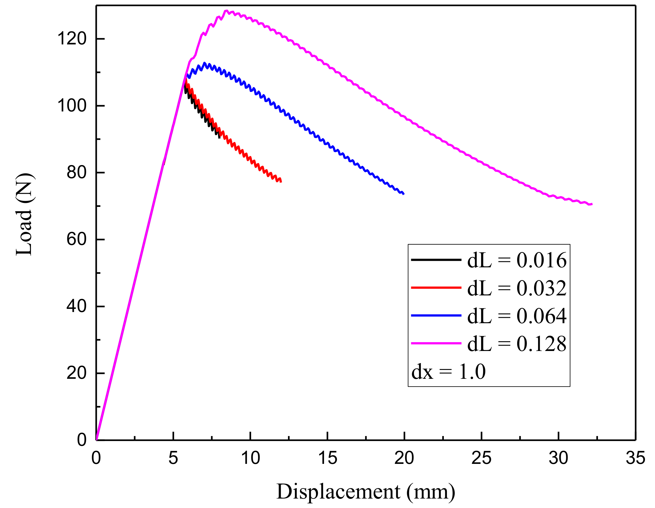
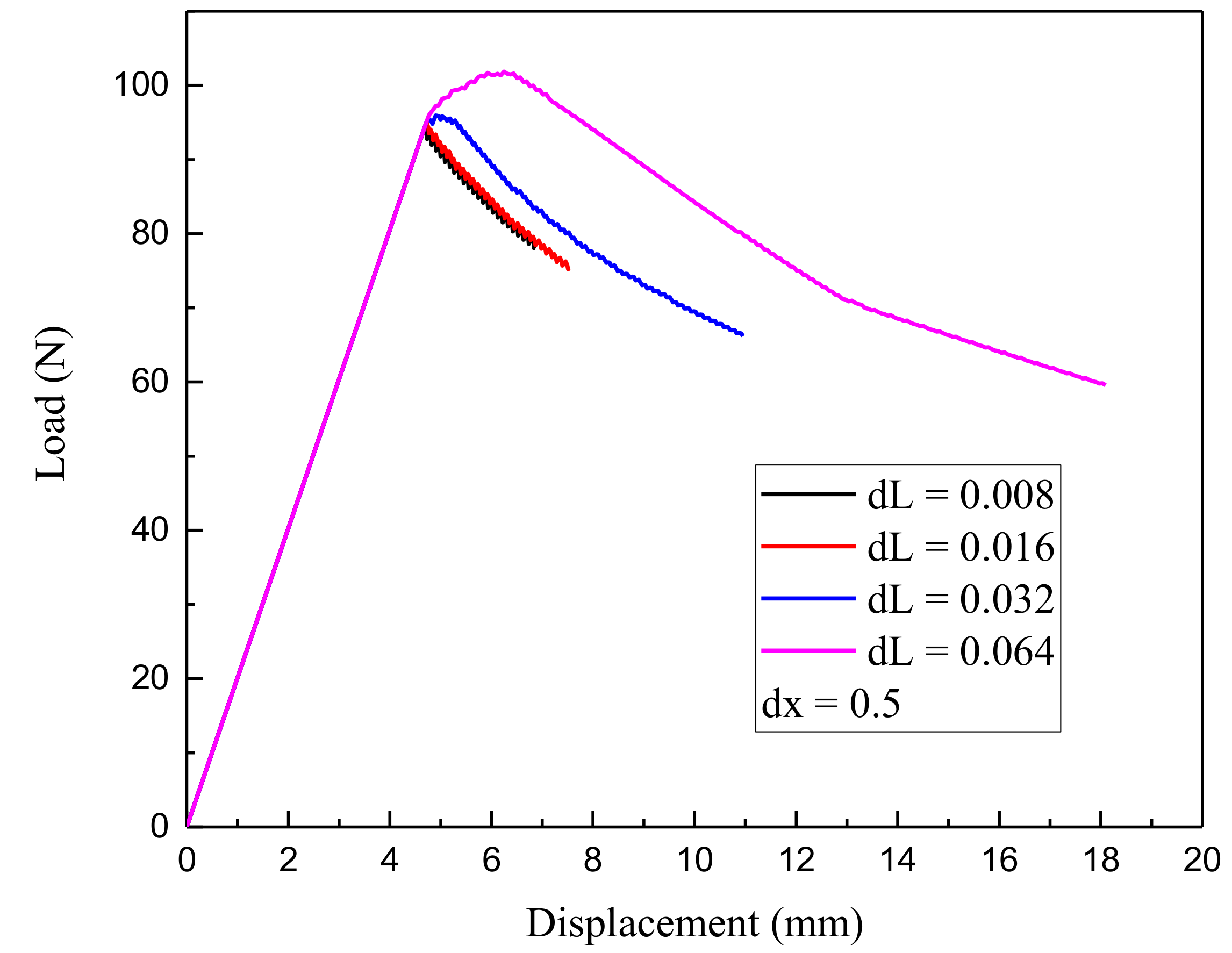
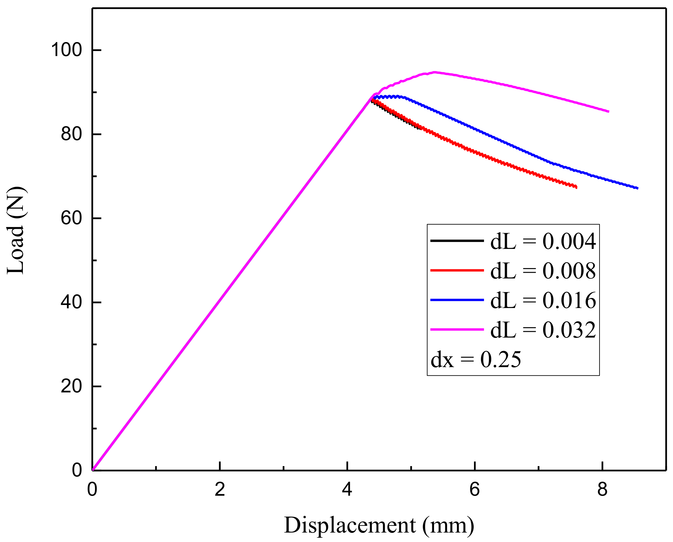
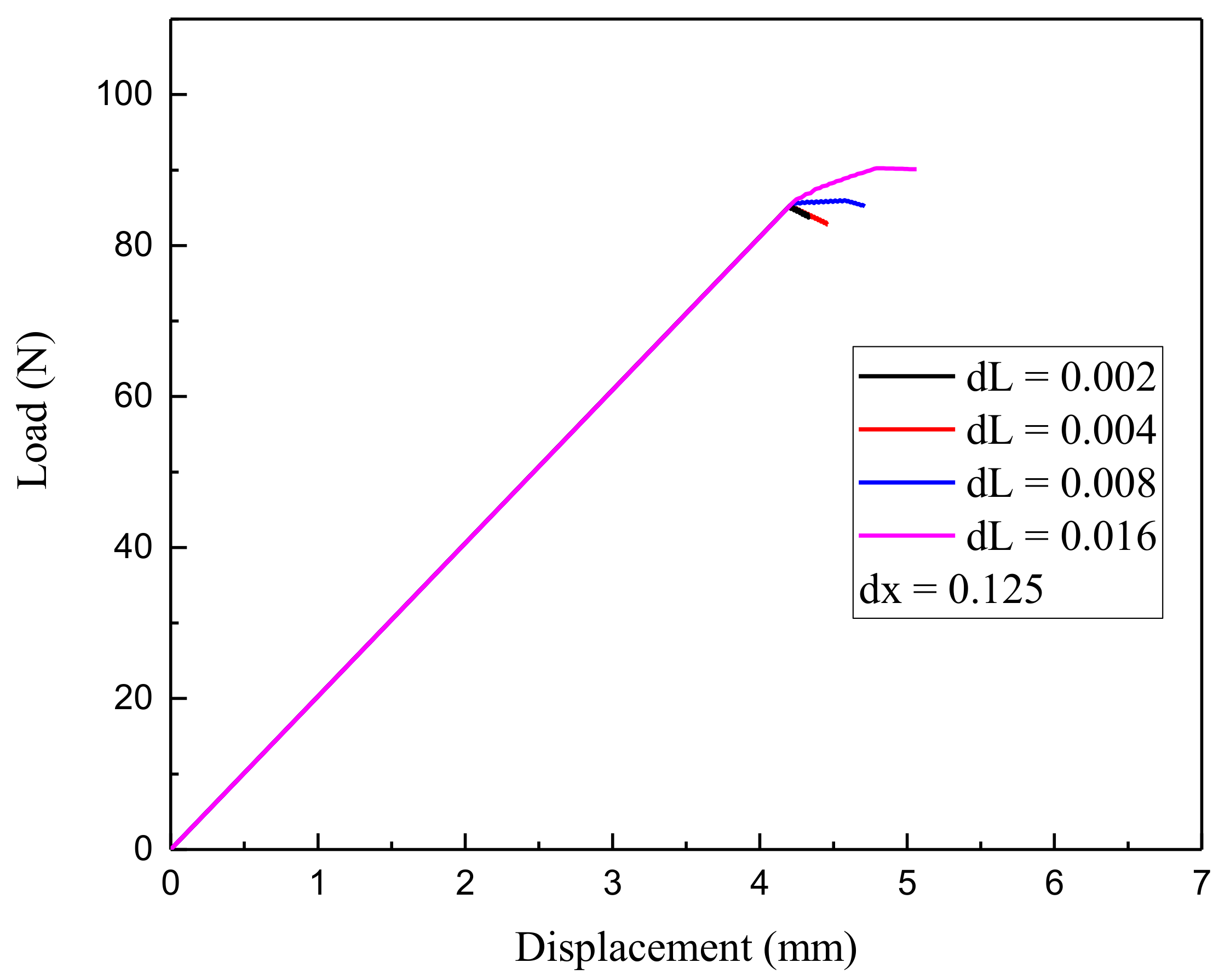
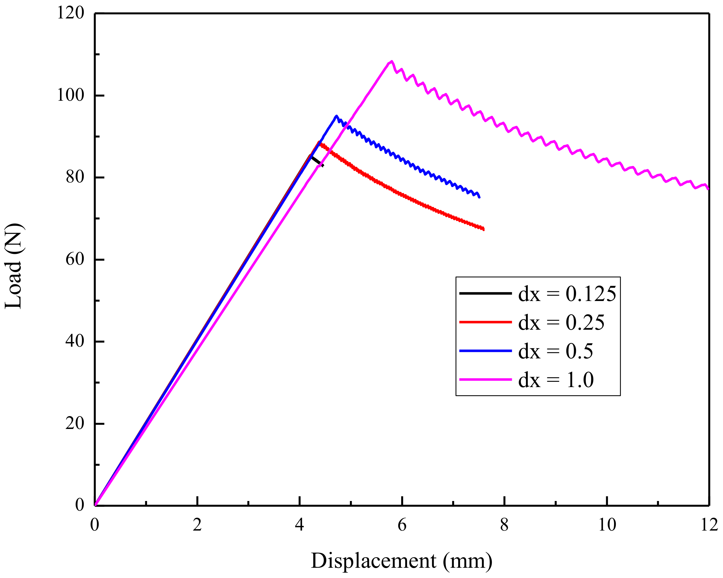
4.1. Loading Increment Convergence Analysis and Grid Spacing Influence Study

In order to investigate the reliability of the present modeling, loading increment convergence analysis and grid spacing influence study are conducted. Four different grid spacing dx are studied: 1.0, 0.5, 0.25, and 0.125 (mm). For each grid spacing, four different loading increments dL are studied:

(1)

For dx = 1.0, dL: 0.128, 0.064, 0.032, 0.016 (mm);

(2)

For dx = 0.5, dL: 0.064, 0.032, 0.016, 0.008 (mm);

(3)

For dx = 0.25, dL: 0.032, 0.016, 0.008, 0.004 (mm);

(4)

For dx = 0.125, dL: 0.016, 0.008, 0.004, 0.002 (mm).

Firstly, loading increment convergence analysis for each grid spacing dx was conducted, as shown in Figure 7, Figure 8, Figure 9 and Figure 10. It can be seen that with the decrease of loading increment dL, the PD modeling load–displacement curve converges for all grid spacing. As expected, the slope of the linear load–displacement part is not influenced by the loading increment, and the loading increment only influences the peak force value for a fixed grid spacing.

Then, the influence of grid spacing was studied in Figure 11. The second least loading increment, dL, was used for each grid spacing. For example, dL = 0.008 mm was used for grid spacing dx = 0.25 mm. It can be seen that with the decrease of grid spacing, the linear loading part of the PD modeling load–displacement curve converges. However, PD modeling delamination growth initial point of load–displacement curve seems sensitive to grid spacing. Similar mesh sensitivity of PD modeling can be found in the work by Beckmann et al. [34], Henke et al. [35], and Steward et al. [36]. In the present study, in order to balance the computation reliability and efficiency, dx = 0.25 mm and dL = 0.008 mm are used in the following discussion.

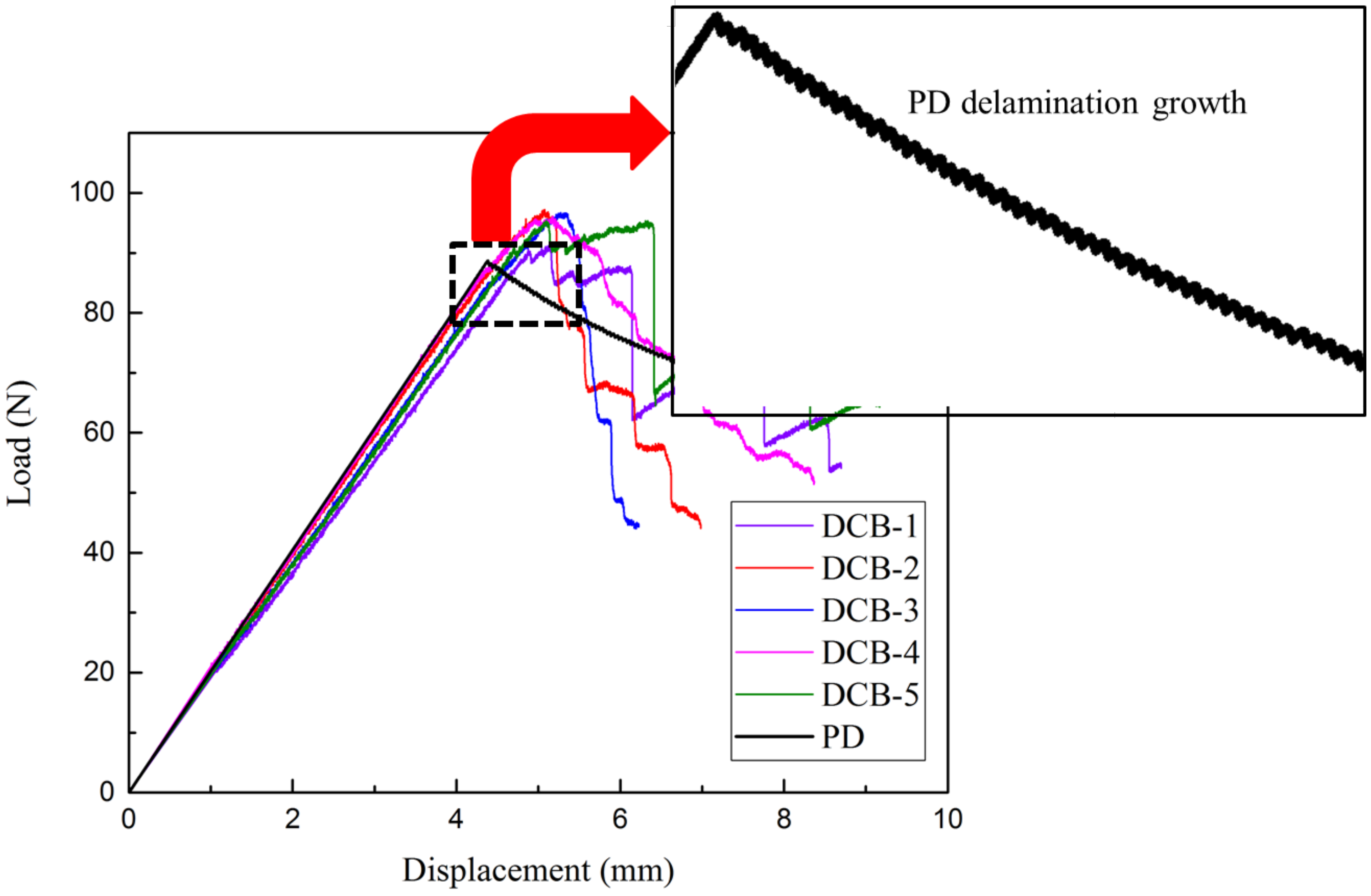
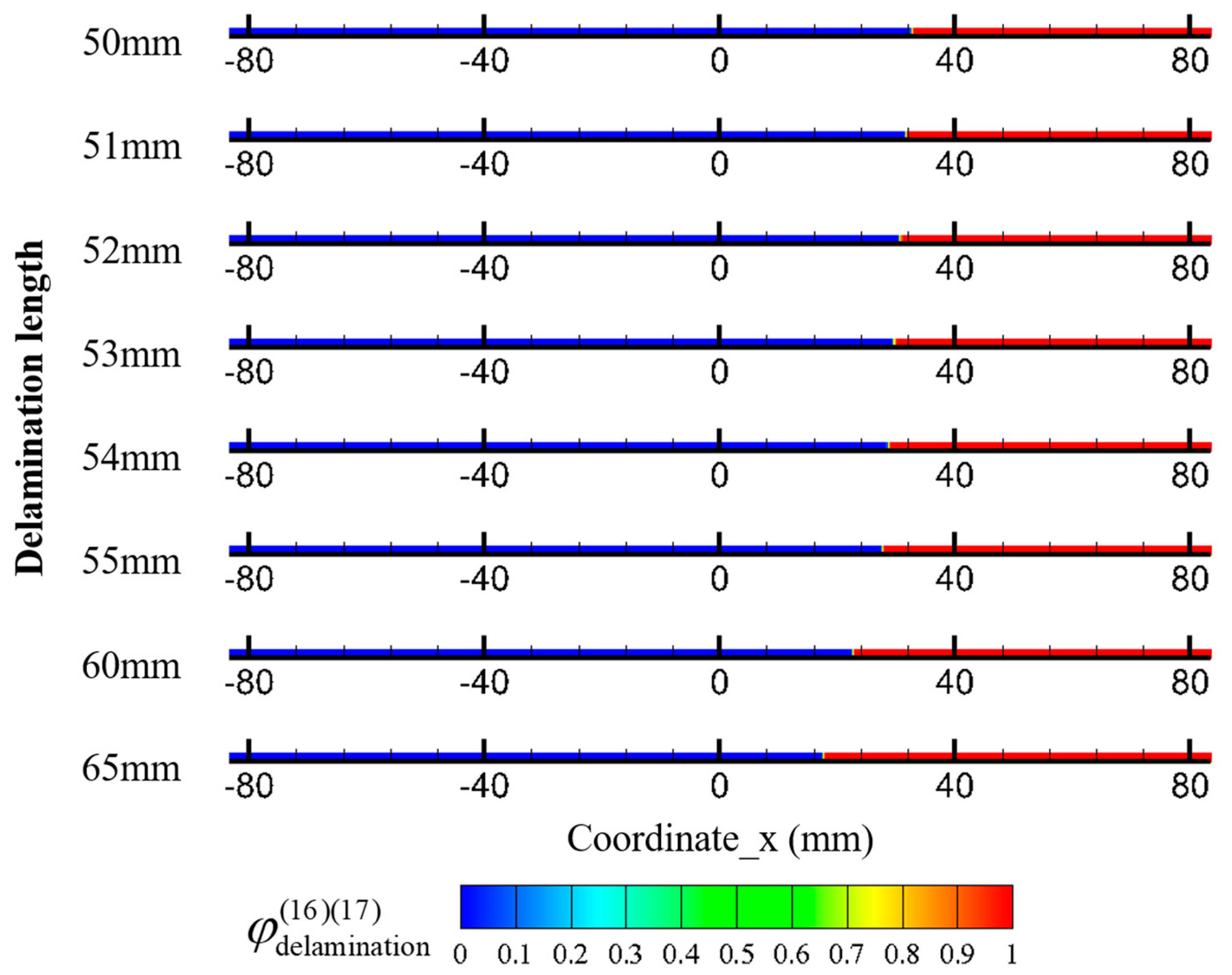
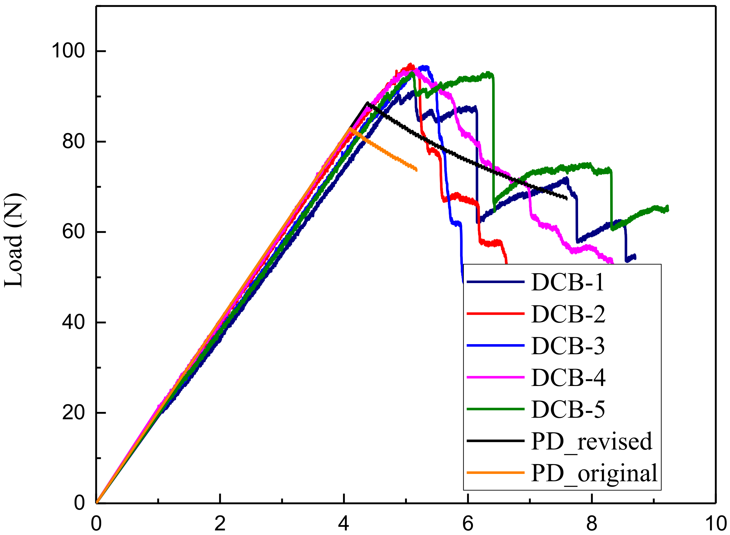
4.2. Comparison of Load–Displacement Curve and Delamination Growth Process

The DCB load–displacement curve of the PD and experimental results are compared as shown in Figure 12. The load–displacement curve of PD delamination growth is shown in Figure 13. The results in Figure 12 show that the PD-based analytical result agrees well with experimental results. It is also noted that the modeling load–displacement curve of PD delamination growth shows a zigzag-shaped curve in Figure 13. This is due to the fact that when the delamination front grows for a grid spacing, the displacement-controlled load will drop. Before the next delamination front growth happens, the load will slightly increase with the increase of displacement. A similar phenomenon is also observed in the load–displacement curves obtained from experiments, as shown in Figure 12. However, due to the complex specimen manufacturing process, preset delamination condition, and experimental setup condition, the load–displacement curve obtained from experiments show significant discrepancy between different specimens.

Quantitative delamination growth process is also compared between PD and experiment as presented in

Table 3. Comparison between PD delamination growth with experimental average results (DELL: delamination length).

DELL (mm)	Experimental Avg.		PD		Difference
	Disp. (mm)	Load (N)	Disp. (mm)	Load (N)	Disp. (mm)	Load (N)
50	5.09	91.35	4.39	88.66	−13.78%	−2.95%
51	5.30	87.66	4.55	87.16	−14.10%	−0.57%
52	5.43	85.07	4.72	85.64	−13.00%	0.67%
53	5.49	85.23	4.89	84.13	−11.00%	−1.30%
54	5.52	84.14	5.06	82.62	−8.29%	−1.81%
55	5.70	81.99	5.23	81.24	−8.26%	−0.91%
60	6.09	67.14	6.16	75.05	1.16%	11.78%
65	6.84	63.64	7.16	69.72	4.66%	9.55%

, and the delamination growth process damage contours are illustrated in Figure 14. In Table 3, the average delamination growth process of the five DCB test samples from 50 (initial delamination) to 65 mm (shown in Table 1) is compared with the modeling results. From the results, it noted that the present PD simulation results for the composite DCB delamination growth process agree well with the experimental results. The maximum difference between PD and experimental average results in displacement is −14.10%, and is 11.78% in load. In Figure 14, the delamination damage coefficient ${\phi }_{\mathrm{delamination}}^{(16)(17)}$ is calculated using Equation (24). The delamination length growing from 50 (initial delamination) to 65 mm is vividly shown. It is worth noting that the PD delamination growth process shown in Figure 14 is “spontaneous”. It does not need presetting of delamination path, nor non-physical stabilization parameters which are required for FEM modeling [26]. Also, it does not require the refinement of delamination front grid spacing.

4.3. Comparison of Numerical Modeling Using Revised and Original Energy-Based Failure Criteria

In order to investigate the influence of the revised energy-based failure criteria proposed in Section 2.2, a comparison study is conducted by modeling the DCB delamination using the revised and original energy-based failure criteria. The revised energy-based failure criteria are illustrated in Equation (22). And the original energy-based failure criteria [15] for two-dimensional modeling are

$$\left|\frac{w_{\mathrm{I}}}{w_{\mathrm{IC}}}\right|\ge 1, w_{\mathrm{IC}}=\frac{G_{\mathrm{IC}}}{\frac{4}{3}{\delta }^3}, w_{\mathrm{I}}=t_z(w^{\prime }-w).$$

(31)

The modeling load–displacement curve using revised and original energy-based failure criteria, as well as the experimental results, are shown in Figure 15. The comparison of maximum load using the revised and original energy-based failure criteria and the average experimental results are presented in

Table 4. Influence of the revised bond energy-based failure criteria on maximum load.

Comparison	Experimental Avg.	PD_original	PD_revised
Max load	95.29	82.97	88.66
Difference	/	−12.93%	−6.96%

.

From Figure 15, it is observed that the modeling load–displacement curve using revised and original energy-based failure criteria overlapped each other before delamination initiation. However, the modeling delamination initiation was delayed using the revised energy-based failure criteria, which agrees more closely with the experimental results. As shown in Table 4, the differences in the maximum load of the modeling load–displacement curve in comparison with the average experimental results was reduced from −12.93% to −6.96% by using the revised energy-based failure criteria. The above results show that the revised energy-based failure criteria can significantly improve the accuracy of the PD delamination modeling of DCB test.

5. Conclusions

In this study, a two-dimensional ordinary state-based peridynamic (OSB PD) modeling of mode-I delamination growth in double cantilever composite beam (DCB) test is conducted. The two-dimensional OSB PD composite model for DCB modeling is obtained by reformulating the previous OSB PD lamina model in x–z direction. Additionally, revised energy-based failure criteria are proposed for modeling delamination initiation and growth.

In order to investigate the reliability of current modeling, loading increment convergence analysis and grid spacing influence study are conducted. It is shown that the PD modeling load–displacement curve converges with the decrease of loading increment. The linear loading part of PD modeling load–displacement curve converges with the decrease of grid spacing. However, the delamination growth initial point of PD modeling load–displacement curve seems sensitive to grid spacing, similar to the previous literature work.

The standard DCB test was performed with five composite DCB specimens to measure the mode-I delamination fracture toughness G_IC. The load–displacement variation and delamination growths were also measured. The modeling load–displacement curve and delamination growth process using the present PD model are then compared with experimental results. The results show that the PD-based load–displacement curve agrees well with experimental results. The zigzag load–displacement curve for delamination growth was observed both in experimental results and the present PD modeling results. Well agreement of the PD modeling delamination growth progress with experimental results is achieved. In particular, the maximum difference between PD and experimental average results in displacement is −14.10%, and in load is 11.78%. Besides, the PD modeling delamination growth process damage contours are illustrated.

To demonstrate the influence of the revised energy-based failure criteria, a comparison study using the revised and original energy-based failure criteria in the PD modeling is conducted. It is shown that the modeling delamination initiation was delayed using the revised energy-based failure criteria, which agrees more closely with the experimental results. In particular, by using the revised energy-based failure criteria, the differences with experimental results in the maximum load of the modeling load–displacement curve was reduced from −12.93% to −6.96%, which show significant improvement in the accuracy of delamination modeling of DCB test.

References

1. Alfano, G.; Crisfield, M.A. Finite element interface models for the delamination analysis of laminated composites: Mechanical and computational issues. Int. J. Numer. Methods Eng. 2001, 50, 1701–1736. [Google Scholar] [CrossRef]
2. Camanho, P.P.; Vila, C.G.D.; Ambur, D.R. Numerical Simulation of Delamination Growth in Composite Materials; NASA Technical Paper 211041; NASA: Washington, DC, USA, 2001; pp. 1–24.
3. Camanho, P.P.; Dávila, C.G.; De Moura, M.F. Numerical simulation of mixed-mode progressive delamination in composite materials. J. Compos. Mater. 2003, 37, 1415–1438. [Google Scholar] [CrossRef]
4. Meo, M.; Thieulot, E. Delamination modelling in a double cantilever beam. Compos. Struct. 2005, 71, 429–434. [Google Scholar] [CrossRef]
5. Zhao, L.; Zhi, J.; Zhang, J.; Liu, Z.; Hu, N. XFEM simulation of delamination in composite laminates. Compos. Part A Appl. Sci. Manuf. 2016, 80, 61–71. [Google Scholar] [CrossRef]
6. Kim, S.H.; Kim, C.G. Optimal design of composite stiffened panel with cohesive elements using micro-genetic algorithm. J. Compos. Mater. 2008, 42, 2259–2273. [Google Scholar] [CrossRef]
7. Orifici, A.C.; Shah, S.A.; Herszberg, I.; Kotler, A.; Weller, T. Failure analysis in postbuckled composite T-sections. Compos. Struct. 2008, 86, 146–153. [Google Scholar] [CrossRef]
8. Riccio, A.; Raimondo, A.; Di Felice, G.; Scaramuzzino, F. A numerical procedure for the simulation of skin-stringer debonding growth in stiffened composite panels. Aerosp. Sci. Technol. 2014, 39, 307–314. [Google Scholar] [CrossRef]
9. Oterkus, E.; Madenci, E. Peridynamic Theory for Damage Initiation and Growth in Composite Laminate. Key Eng. Mater. 2012, 488–489, 355–358. [Google Scholar] [CrossRef]
10. Xu, J.; Askari, A.; Weckner, O.; Silling, S. Peridynamic Analysis of Impact Damage in Composite Laminates. J. Aerosp. Eng. 2008, 21, 187–194. [Google Scholar] [CrossRef]
11. Askari, E.; Xu, J.; Silling, S. Peridynamic Analysis of Damage and Failure in Composites. In Proceedings of the 44th AIAA Aerospace Sciences Meeting and Exhibit, Reno, NV, USA, 9–12 January 2006; American Institute of Aeronautics and Astronautics: Reston, VA, USA, 2006; pp. 1–12. [Google Scholar]
12. Hu, Y.L.; De Carvalho, N.V.; Madenci, E. Peridynamic modeling of delamination growth in composite laminates. Compos. Struct. 2015, 132, 610–620. [Google Scholar] [CrossRef]
13. Silling, S.A.; Epton, M.; Weckner, O.; Xu, J.; Askari, E. Peridynamic states and constitutive modeling. J. Elast. 2007, 88, 151–184. [Google Scholar] [CrossRef]
14. Silling, S.A. Reformulation of elasticity theory for discontinuities and long-range forces. J. Mech. Phys. Solids 2000, 48, 175–209. [Google Scholar] [CrossRef] [Green Version]
15. Silling, S.A.; Lehoucq, R.B. Peridynamic Theory of Solid Mechanics. In Advances in Applied Mechanics; Aref, H., VanDerGiessen, E., Eds.; Elsevier: Amsterdam, The Netherlands, 2010; pp. 73–168. [Google Scholar]
16. Diyaroglu, C.; Oterkus, E.; Madenci, E.; Rabczuk, T.; Siddiq, A. Peridynamic modeling of composite laminates under explosive loading. Compos. Struct. 2016, 144, 14–23. [Google Scholar] [CrossRef] [Green Version]
17. Oterkus, E.; Madenci, E. Peridynamic Analysis of Fiber Reinforced Composite Materials. J. Mech. Mater. Struct. 2012, 7, 45–84. [Google Scholar] [CrossRef]
18. Oterkus, E.; Madenci, E.; Weckner, O.; Silling, S.; Bogert, P.; Tessler, A. Combined finite element and peridynamic analyses for predicting failure in a stiffened composite curved panel with a central slot. Compos. Struct. 2012, 94, 839–850. [Google Scholar] [CrossRef]
19. Oterkus, E.; Barut, A.; Madenci, E. Damage Growth Prediction from Loaded Composite Fastener Holes by Using Peridynamic Theory. In Proceedings of the 51th AIAA/ASME/ASCE/AHS/ASC Structures, Structural Dynamics, and Materials Conference, Orlando, FL, USA, 12–15 April 2010. Paper No.2010-3026. [Google Scholar]
20. Hu, Y.; Yu, Y.; Wang, H. Peridynamic analytical method for progressive damage in notched composite laminates. Compos. Struct. 2014, 108, 801–810. [Google Scholar] [CrossRef]
21. Hu, Y.L.; Madenci, E. Bond-based peridynamic modeling of composite laminates with arbitrary fiber orientation and stacking sequence. Compos. Struct. 2016, 153, 139–175. [Google Scholar] [CrossRef]
22. Hu, Y.; Madenci, E.; Phan, N.D. Peridynamics for Predicting Tensile and Compressive Strength of Notched Composites. In Proceedings of the 57th AIAA/ASCE/AHS/ASC Structures, Structural Dynamics, and Materials Conference, San Diego, CA, USA, 4–8 January 2016; American Institute of Aeronautics and Astronautics: Reston, VA, USA, 2016. [Google Scholar]
23. Hu, Y.L.; Madenci, E. Peridynamics for fatigue life and residual strength prediction of composite laminates. Compos. Struct. 2017, 160, 169–184. [Google Scholar] [CrossRef]
24. Heidari-Rarani, M.; Shokrieh, M.M.; Camanho, P.P. Finite element modeling of mode I delamination growth in laminated DCB specimens with R-curve effects. Compos. Part B Eng. 2013, 45, 897–903. [Google Scholar] [CrossRef]
25. Shanmugam, V.; Penmetsa, R.; Tuegel, E.; Clay, S. Stochastic modeling of delamination growth in unidirectional composite DCB specimens using cohesive zone models. Compos. Struct. 2013, 102, 38–60. [Google Scholar] [CrossRef]
26. Krueger, R. A summary of benchmark examples to assess the performance of quasi-static delamination propagation prediction capabilities in finite element codes. J. Compos. Mater. 2015, 49, 3297–3316. [Google Scholar] [CrossRef]
27. Madenci, E.; Oterkus, E. Peridynamic Theory and Its Applications; Springer: New York, NY, USA, 2014. [Google Scholar]
28. Silling, S.A.; Askari, E. A meshfree method based on the peridynamic model of solid mechanics. Comput. Struct. 2005, 83, 1526–1535. [Google Scholar] [CrossRef]
29. Kilic, B.; Madenci, E. An adaptive dynamic relaxation method for quasi-static simulations using the peridynamic theory. Theor. Appl. Fract. Mech. 2010, 53, 194–204. [Google Scholar] [CrossRef]
30. Breitenfeld, M.S.; Geubelle, P.H.; Weckner, O.; Silling, S.A. Non-ordinary state-based peridynamic analysis of stationary crack problems. Comput. Methods Appl. Mech. Eng. 2014, 272, 233–250. [Google Scholar] [CrossRef]
31. Ni, T.; Zaccariotto, M.; Zhu, Q.-Z.; Galvanetto, U. Static solution of crack propagation problems in Peridynamics. Comput. Methods Appl. Mech. Eng. 2019, 346, 126–151. [Google Scholar] [CrossRef]
32. Fatica, M.; Ruetsch, G. CUDA Fortran for Scientists and Engineers: Best Practices for Efficient CUDA Fortran Programming; Elsevier: Amsterdam, The Netherlands, 2013. [Google Scholar]
33. ASTM: D5528-13: Standard Test Method for Mode I Interlaminar Fracture Toughness of Unidirectional Fiber-Reinforced Polymer Matrix Composites; American Society for Testing and Materials: West Conshohocken, PA, USA, 2013.
34. Beckmann, R.; Mella, R.; Wenman, M.R. Mesh and timestep sensitivity of fracture from thermal strains using peridynamics implemented in Abaqus. Comput. Methods Appl. Mech. Eng. 2013, 263, 71–80. [Google Scholar] [CrossRef]
35. Henke, S.F.; Shanbhag, S. Mesh sensitivity in peridynamic simulations. Comput. Phys. Commun. 2014, 185, 181–193. [Google Scholar] [CrossRef]
36. Steward, R.J.; Jeon, B. Decoupling strength and grid resolution. In Proceedings of the 18th U.S. National Congress for Theoretical and Applied Mechanics, Chicago, IL, USA, 4–9 June 2018. [Google Scholar]
Figure 1. Peridynamic model notations.
Applsci 09 00656 g001
Figure 2. Computation of total energy absorbed by P for delamination front area a.
Applsci 09 00656 g002
Figure 3. Carbon fiber-reinforced polymer (CFRP) double cantilever beam (DCB) test and two-dimensional PD modeling. (a) Double cantilever composite beam (DCB) test setup, (b) peridynamic (PD) modeling deformed displacement field in thickness direction (mm).
Applsci 09 00656 g003
Figure 4. CFRP double cantilever beam (DCB) test specimen.
Applsci 09 00656 g004
Figure 5. Boundary conditions for PD DCB model.
Applsci 09 00656 g005
Figure 6. PD DCB modeling flowchart.
Applsci 09 00656 g006
Figure 7. Convergence analysis of loading increment dL for grid spacing dx = 1.0 mm, PD modeling load–displacement.
Applsci 09 00656 g007
Figure 8. Convergence analysis of loading increment dL for grid spacing dx = 0.5 mm, PD modeling load–displacement.
Applsci 09 00656 g008
Figure 9. Convergence analysis of loading increment dL for grid spacing dx = 0.25 mm, PD modeling load–displacement.
Applsci 09 00656 g009
Figure 10. Convergence analysis of loading increment dL for grid spacing dx = 0.125 mm, PD modeling load–displacement.
Applsci 09 00656 g010
Figure 11. Influence of different grid spacing, PD modeling load–displacement.
Applsci 09 00656 g011
Figure 12. Comparison of load–displacement curve between DCB test and PD (dx = 0.25 mm, dL = 0.008 mm).
Applsci 09 00656 g012
Figure 13. Zigzag-shaped load–displacement curve of DCB test delamination growth process.
Applsci 09 00656 g013
Figure 14. PD modeling delamination growth process damage contours on the mid-plane of DCB specimen, between Layer 16 and 17.
Applsci 09 00656 g014
Figure 15. Comparison of load–displacement curve obtained using revised and original bond energy-based failure criteria.
Applsci 09 00656 g015