Hierarchical Optimization Method for Energy Scheduling of Multiple Microgrids


Abstract
:1. Introduction
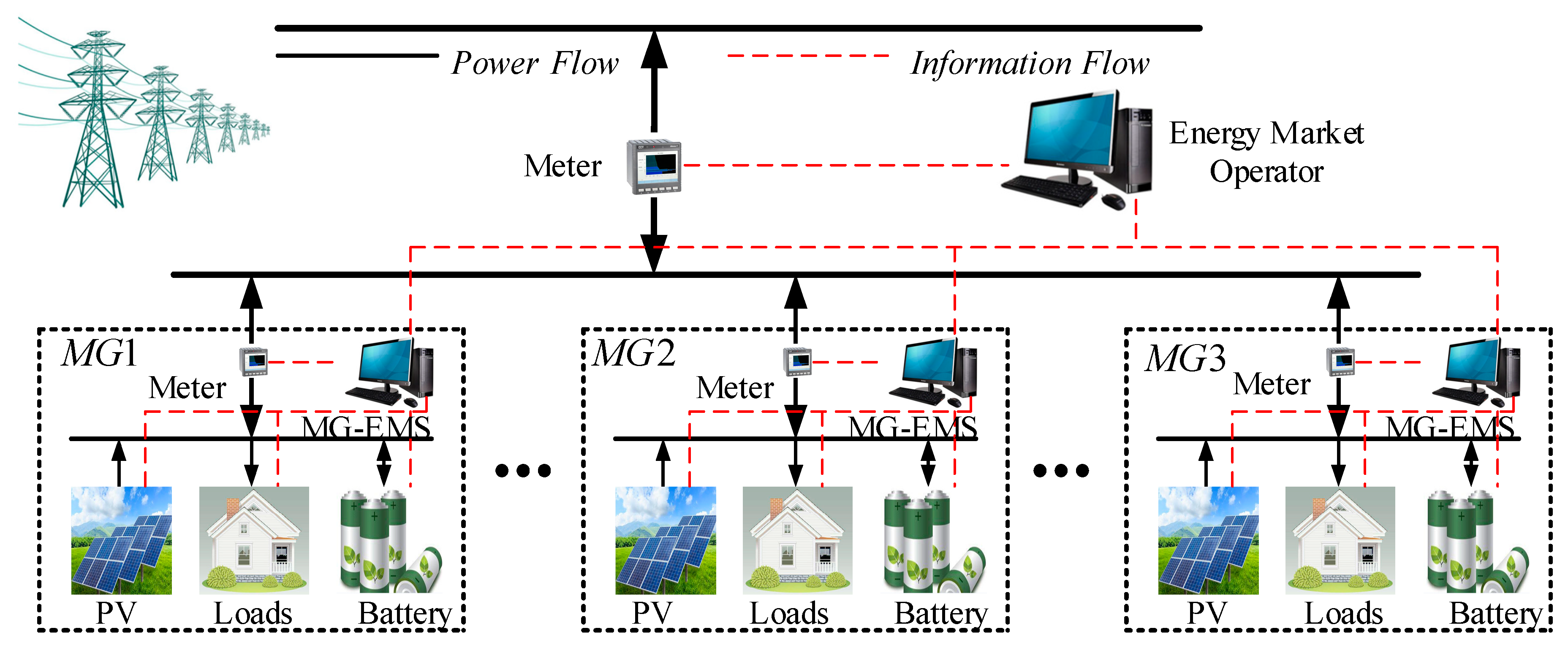
2. Framework
2.1. Structure of an MMG
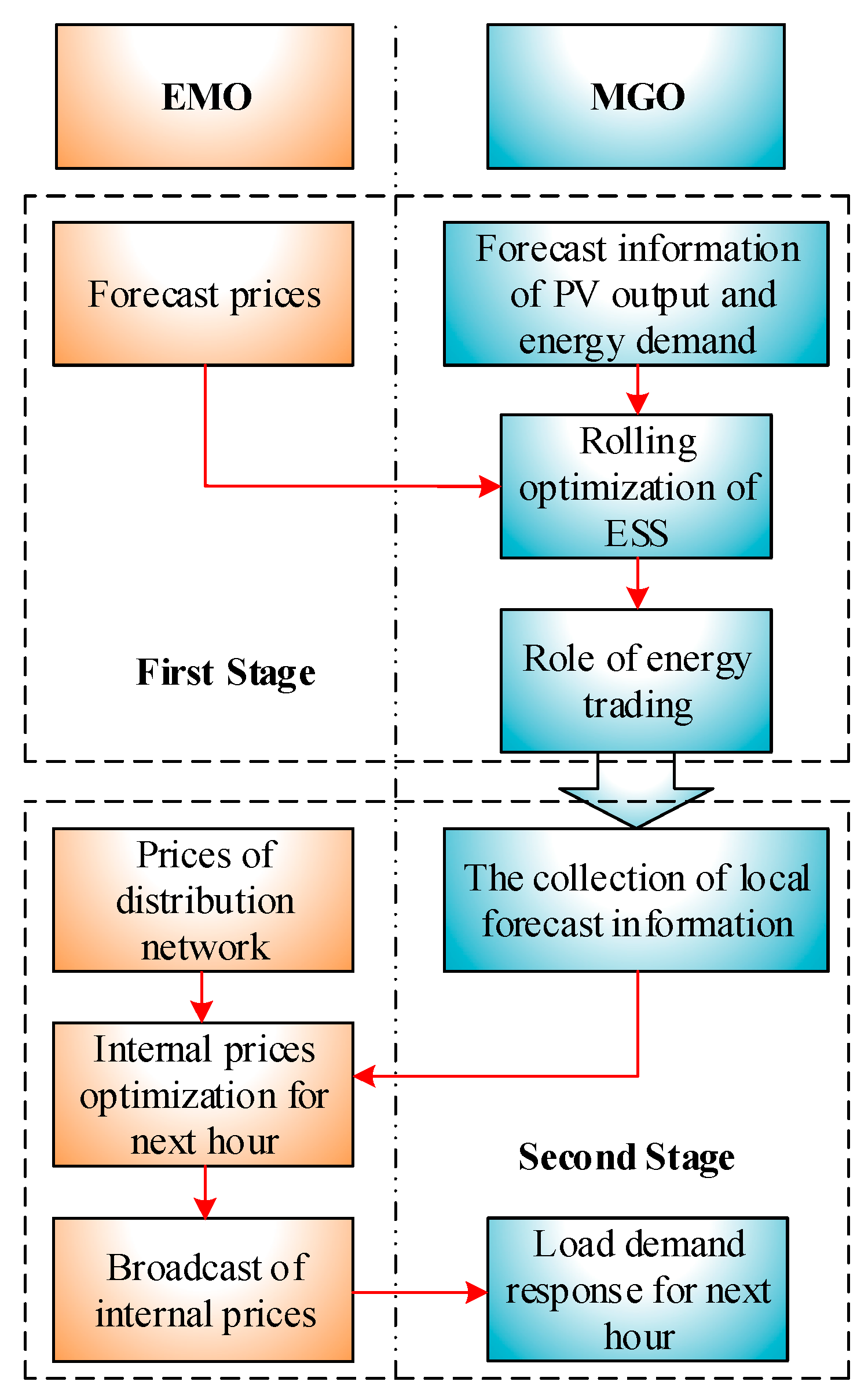
2.2. Operation Strategy
2.2.1. First Stage
2.2.2. Second Stage
3. System Model
3.1. Utility Model of MGs
3.2. Profit Model of EMOs
4. Optimization Scheduling
4.1. Rolling Optimization for Local MGs
4.2. Stackelberg Game for EMOs
4.2.1. Formulation of a Stackelberg Game
4.2.2. Achievement of Game Equilibrium
5. Case Studies
5.1. Basic Data
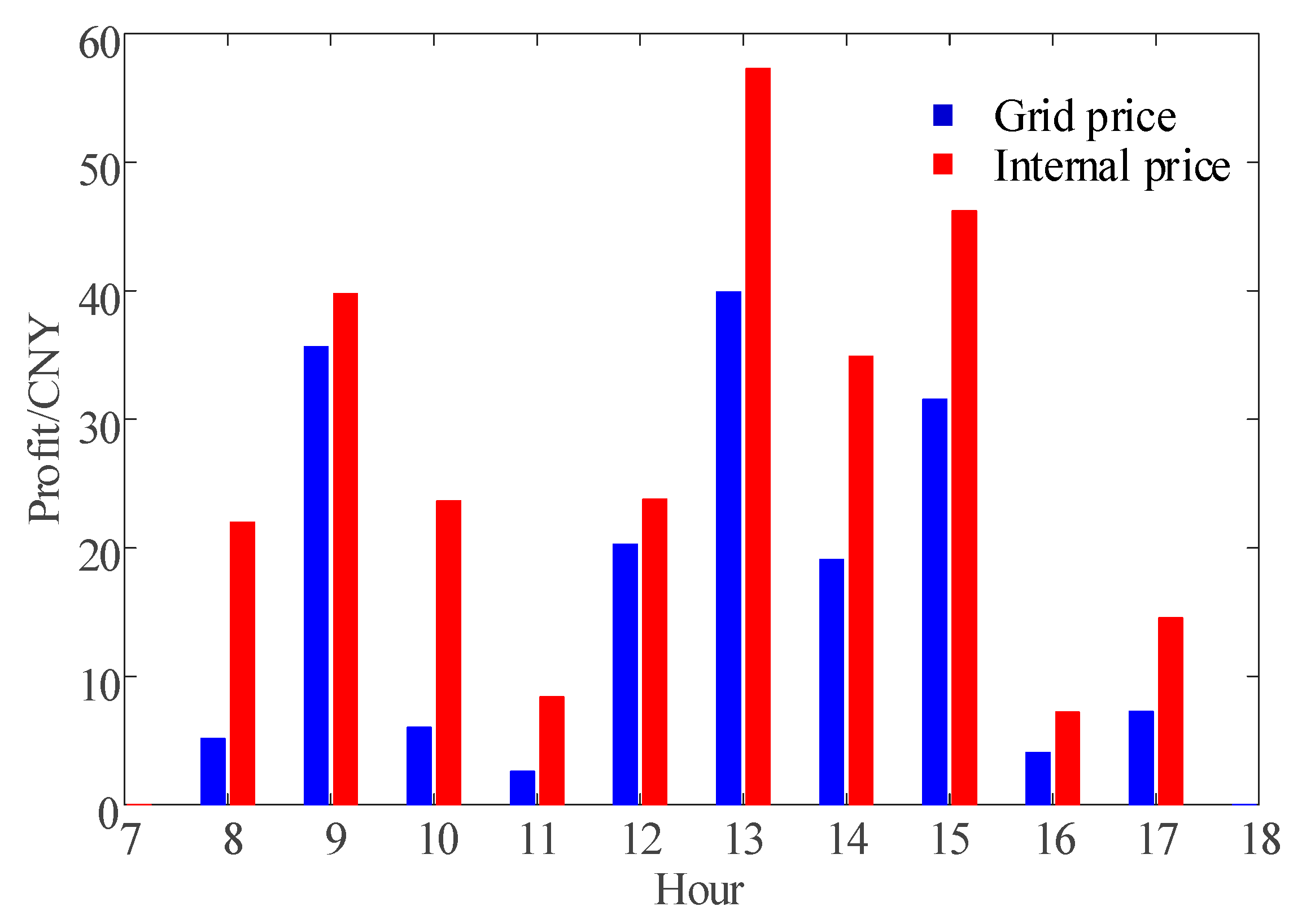
5.2. Internal Prices of the MMG
5.3. Results of Local MGs
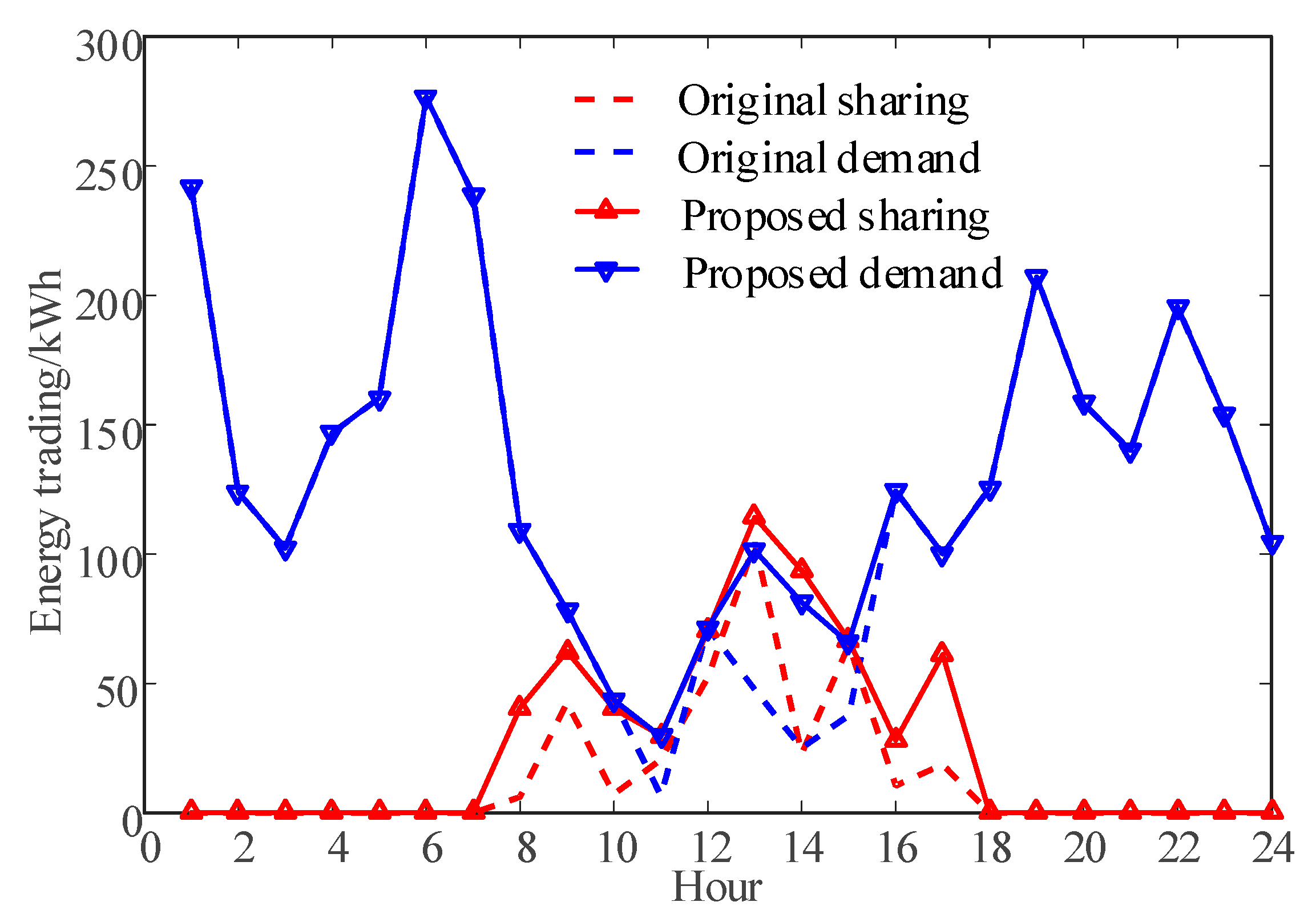
5.3.1. Rolling Optimization of ESSs
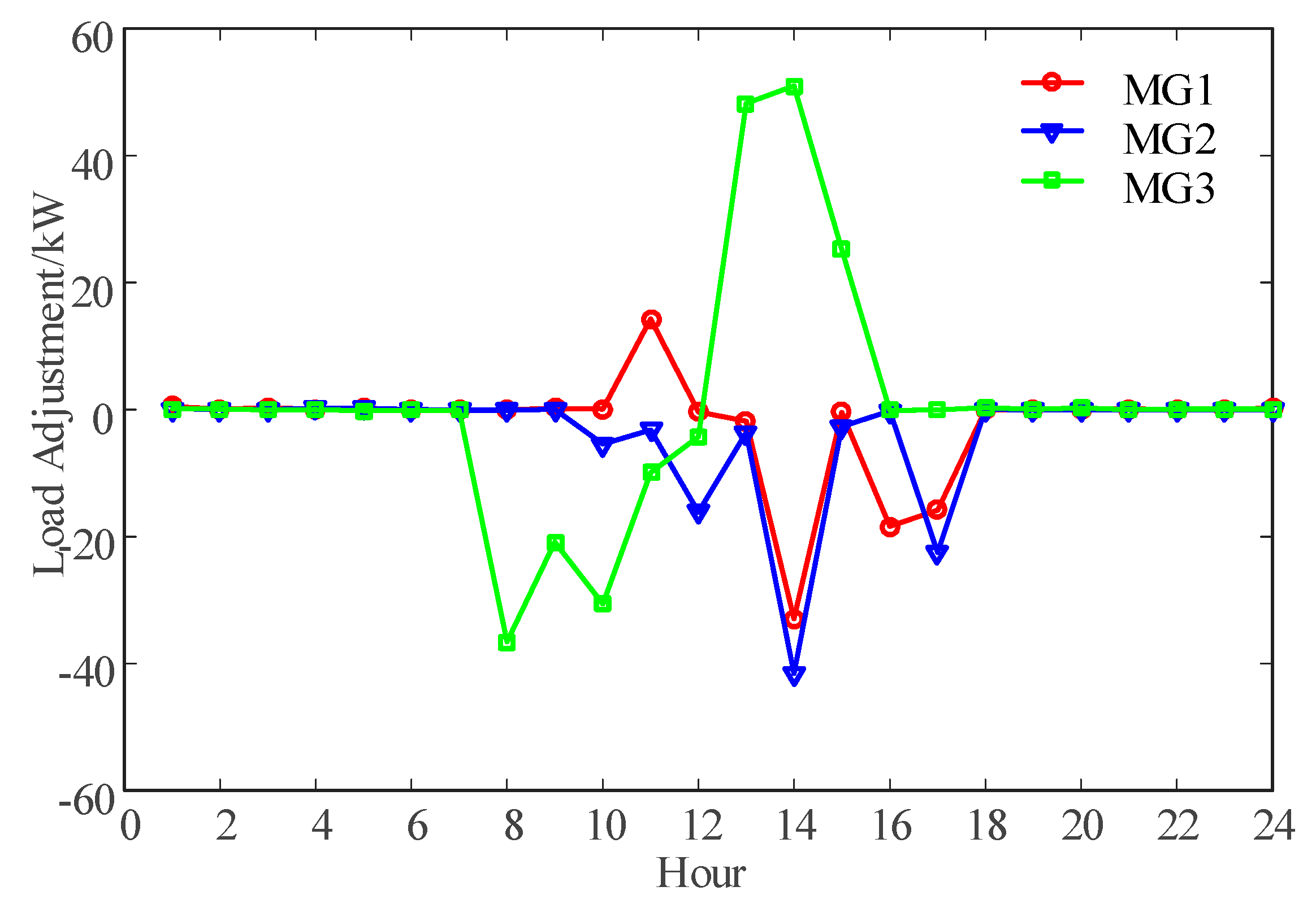
5.3.2. Demand Response of Local MGs
5.4. Results of the EMO
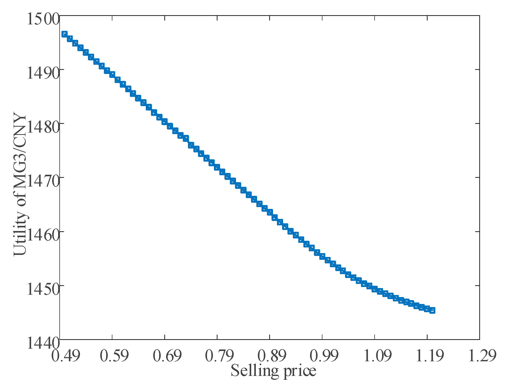
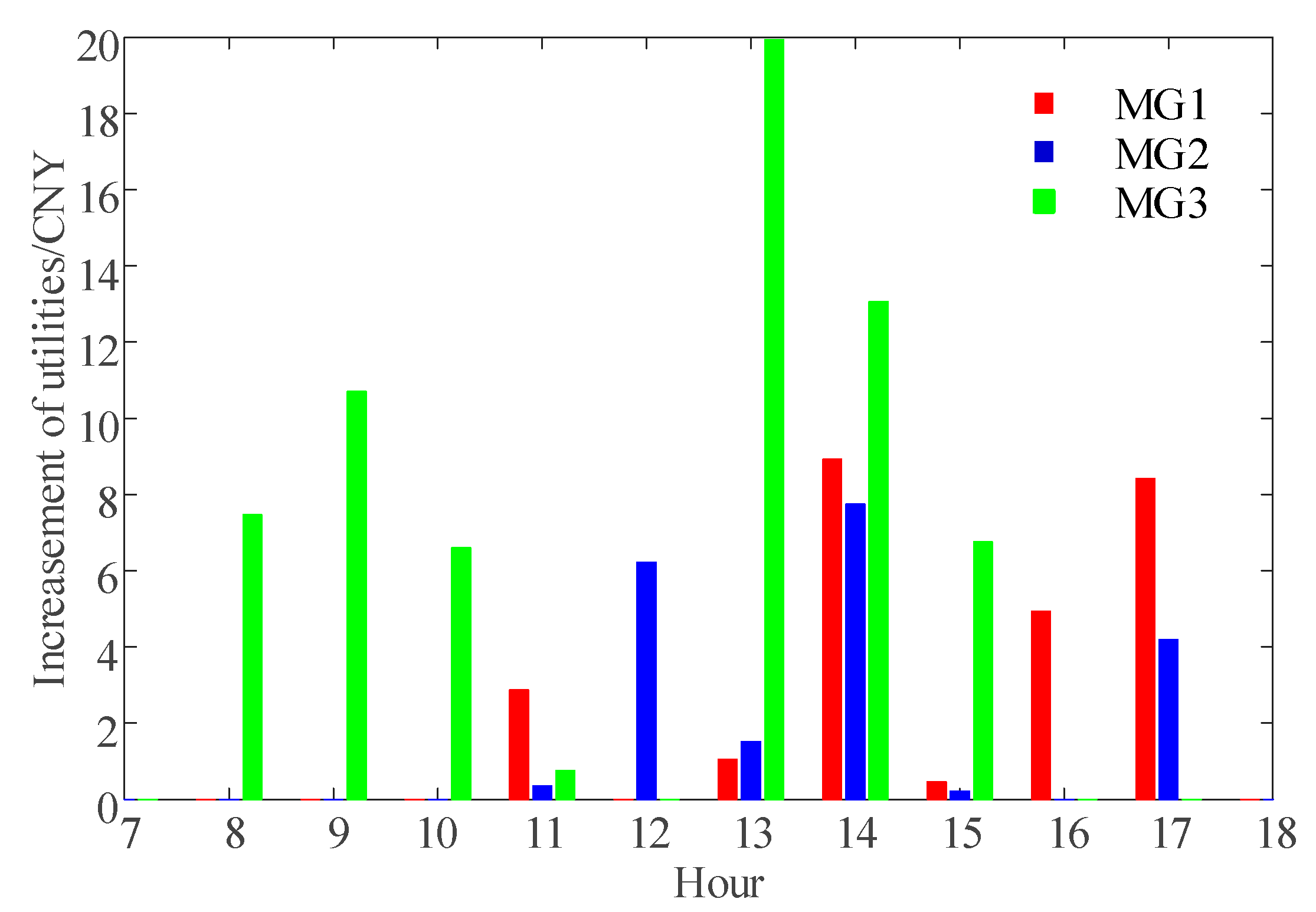
5.5. Utility Comparisons with Other Methods
6. Conclusions
Author Contributions
Funding
Conflicts of Interest
Appendix A
Appendix B


Appendix C

| Period | MG1 | MG2 | >MG3 |
|---|---|---|---|
| 0:00–8:00 | buyer | buyer | buyer |
| 8:00–9:00 | buyer | buyer | seller |
| 9:00–10:00 | buyer | buyer | seller |
| 10:00–11:00 | buyer | buyer | seller |
| 11:00–12:00 | buyer | buyer | seller |
| 12:00–13:00 | buyer | seller | buyer |
| 13:00–14:00 | seller | seller | buyer |
| 14:00–15:00 | seller | seller | buyer |
| 15:00–16:00 | seller | seller | buyer |
| 16:00–17:00 | seller | buyer | buyer |
| 17:00–18:00 | seller | seller | buyer |
| 18:00–24:00 | buyer | buyer | buyer |
References
- Rafique, S.F.; Zhang, J. Energy management system, generation and demand predictors: A review. IET Gener. Transm. Distrib. 2018, 7, 519–530. [Google Scholar] [CrossRef]
- Han, Y.; Zhang, K.; Li, H.; Coelho, E.A.; Guerrero, J.M. MAS-based Distributed Coordinated Control and Optimization in Microgrid and Microgrid Clusters: A Comprehensive Overview. IEEE Trans. Power Electron. 2018, 33, 6488–6508. [Google Scholar] [CrossRef]
- Nguyen, T.A.; Crow, M.L. Stochastic Optimization of Renewable-Based Microgrid Operation Incorporating Battery Operating Cost. IEEE Trans. Power Syst. 2016, 31, 2289–2296. [Google Scholar] [CrossRef]
- Liu, W.; Gu, W.; Sheng, W.; Meng, X.; Wu, Z.; Chen, W. Decentralized Multi-Agent System-Based Cooperative Frequency Control for Autonomous Microgrids With Communication Constraints. IEEE Trans. Sustain. Energy 2014, 5, 446–456. [Google Scholar] [CrossRef]
- Li, Q.; Chen, F.; Chen, M.; Guerrero, J.M.; Abbott, D. Agent-Based Decentralized Control Method for Islanded Microgrids. IEEE Trans. Smart Grid 2016, 7, 637–649. [Google Scholar] [CrossRef]
- Parisio, A.; Wiezorek, C.; Kyntäjä, T.; Elo, J.; Strunz, K.; Johansson, K.H. Cooperative MPC-Based Energy Management for Networked Microgrids. IEEE Trans. Smart Grid 2017, 8, 3066–3074. [Google Scholar] [CrossRef]
- Najmeh, B.; Ahmadreza, T.; Amjad, A.; Josep, M.G. Optimal operation management of a regionalnetwork of microgrids based on chanceconstrained model predictive control. IET Gener. Transm. Distrib. 2018, 12, 3772–3779. [Google Scholar]
- Rafiee Sandgani, M.; Sirouspour, S. Priority-based Microgrid Energy Management in a Network Environment. IEEE Trans. Sustain. Energy 2018, 9, 980–990. [Google Scholar] [CrossRef]
- Jadhav, A.M.; Patne, N.R.; Guerrero, J.M. A Novel Approach to Neighborhood Fair Energy Trading in a Distribution Network of Multiple Microgrid Clusters. IEEE Trans. Ind. Electron. 2018, 66, 1520–1531. [Google Scholar] [CrossRef]
- Zhang, B.; Li, Q.; Wang, L.; Feng, W. Robust optimization for energy transactions in multi-microgrids under uncertainty. Appl. Energy 2018, 217, 346–360. [Google Scholar] [CrossRef]
- Bui, V.H.; Hussain, A.; Kim, H.M. A Multiagent-Based Hierarchical Energy Management Strategy for Multi-Microgrids Considering Adjustable Power and Demand Response. IEEE Trans. Smart Grid 2018, 9, 1323–1333. [Google Scholar] [CrossRef]
- Maryam, M.; Hassan, M.; Amjad, A.; Josep, M.G.; Hamid, L. A decentralized robust model for optimal operation of distribution companies with private microgrids. Electr. Power Energy Syst. 2019, 106, 105–123. [Google Scholar]
- Manshadi, S.D.; Khodayar, M.E. A Hierarchical Electricity Market Structure for the Smart Grid Paradigm. IEEE Trans. Smart Grid 2016, 7, 1866–1875. [Google Scholar] [CrossRef]
- Yue, J.; Hu, Z.; Amjad, A.M.; Josep, M.G. A Multi-Market-Driven Approach to Energy Scheduling of Smart Microgrids in Distribution Networks. Sustainability 2019, 11, 301. [Google Scholar] [CrossRef]
- Fan, S.; Ai, Q.; Piao, L. Bargaining-based cooperative energy trading for distribution company and demand response. Appl. Energy 2018, 226, 469–482. [Google Scholar] [CrossRef]
- Liu, Y.; Guo, L.; Wang, C. A robust operation-based scheduling optimization for smart distribution networks with multi-microgrids. Appl. Energy 2018, 228, 130–140. [Google Scholar] [CrossRef]
- Jalali, M.; Zare, K.; Seyedi, H. Strategic decision-making of distribution network operator with multi-microgrids considering demand response program. Energy 2017, 141, 1059–1071. [Google Scholar] [CrossRef]
- Liu, N.; Cheng, M.; Yu, X.; Zhong, J.; Lei, J. Energy Sharing Provider for PV Prosumer Clusters: A Hybrid Approach using Stochastic Programming and Stackelberg Game. IEEE Trans. Ind. Electron. 2018, 65, 6740–6750. [Google Scholar] [CrossRef]
- Liu, N.; Yu, X.; Wang, C.; Wang, J. Energy Sharing Management for Microgrids with PV Prosumers: A Stackelberg Game Approach. IEEE Trans. Ind. Inform. 2017, 13, 1088–1098. [Google Scholar] [CrossRef]
- Abedinia, O.; Amjady, N.; Zareipour, H. A New Feature Selection Technique for Load and Price Forecast of Electrical Power Systems. IEEE Trans. Power Syst. 2017, 32, 62–74. [Google Scholar] [CrossRef]
- Gigoni, L.; Betti, A.; Crisostomi, E. Day-Ahead Hourly Forecasting of Power Generation from Photovoltaic Plants. IEEE Trans. Sustain. Energy 2018, 9, 831–842. [Google Scholar] [CrossRef]


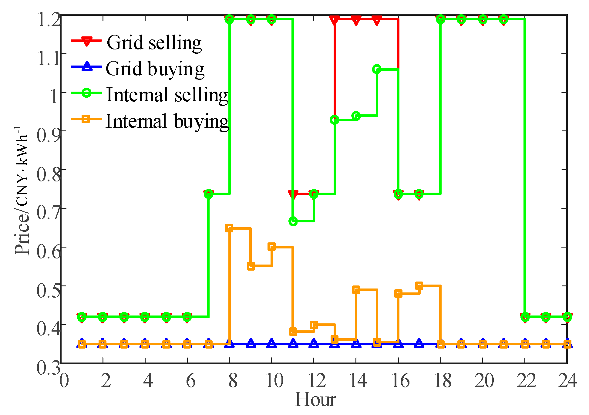
| Distribution Network | Prices (kWh/h) | Hours |
|---|---|---|
| Selling | Peak: 1.189 | 8:00–11:00; 13:00–16:00; 18:00–22:00 |
| Flat: 0.738 | 7:00–8:00; 11:00–13:00; 16:00–18:00 | |
| Valley: 0.423 | 0:00–7:00; 22:00–24:00 | |
| Buying | 0.352 | 0:00–24:00 |
| Method | PAR | PV Utilization Ratio |
|---|---|---|
| Original method | 3.1596 | 85.25% |
| Proposed method | 2.6992 | 98.07% |
© 2019 by the authors. Licensee MDPI, Basel, Switzerland. This article is an open access article distributed under the terms and conditions of the Creative Commons Attribution (CC BY) license (http://creativecommons.org/licenses/by/4.0/).
Share and Cite
Rui, T.; Li, G.; Wang, Q.; Hu, C.; Shen, W.; Xu, B. Hierarchical Optimization Method for Energy Scheduling of Multiple Microgrids. Appl. Sci. 2019, 9, 624. https://doi.org/10.3390/app9040624
Rui T, Li G, Wang Q, Hu C, Shen W, Xu B. Hierarchical Optimization Method for Energy Scheduling of Multiple Microgrids. Applied Sciences. 2019; 9(4):624. https://doi.org/10.3390/app9040624
Chicago/Turabian StyleRui, Tao, Guoli Li, Qunjing Wang, Cungang Hu, Weixiang Shen, and Bin Xu. 2019. "Hierarchical Optimization Method for Energy Scheduling of Multiple Microgrids" Applied Sciences 9, no. 4: 624. https://doi.org/10.3390/app9040624
APA StyleRui, T., Li, G., Wang, Q., Hu, C., Shen, W., & Xu, B. (2019). Hierarchical Optimization Method for Energy Scheduling of Multiple Microgrids. Applied Sciences, 9(4), 624. https://doi.org/10.3390/app9040624