Abstract
This paper discusses the issue of the influence of cartographic Terrestrial Laser Scanning (TLS) data conversion into feature-based automatic registration. Automatic registration of data is a multi-stage process, it is based on original software tools and consists of: (1) Conversion of data to the raster form, (2) register of TLS data in pairs in all possible combinations using the SURF (Speeded Up Robust Features) and FAST (Features from Accelerated Segment Test) algorithms, (3) the quality analysis of relative orientation of processed pairs, and (4) the final bundle adjustment. The following two problems, related to the influence of the spherical image, the orthoimage and the Mercator representation of the point cloud, are discussed: The correctness of the automatic tie points detection and distribution and the influence of the TLS position on the completeness of the registration process and the quality assessment. The majority of popular software applications use manually or semi-automatically determined corresponding points. However, the authors propose an original software tool to address the first issue, which automatically detects and matches corresponding points on each TLS raster representation, utilizing different algorithms (SURF and FAST). To address the second task, the authors present a series of analyses: The time of detection of characteristic points, the percentage of incorrectly detected points and adjusted characteristic points, the number of detected control and check points, the orientation accuracy of control and check points, and the distribution of control and check points. Selection of an appropriate method for the TLS point cloud conversion to the raster form and selection of an appropriate algorithm, considerably influence the completeness of the entire process, and the accuracy of data orientation. The results of the performed experiments show that fully automatic registration of the TLS point clouds in the raster forms is possible; however, it is not possible to propose one, universal form of the point cloud, because a priori knowledge concerning the scanner positions is required. If scanner stations are located close to one another in raster images or in spherical images, Mercator projections are recommended. In the case where fragments of the surface are measured under different angles from different distances and heights of the TLS, orthoimages are suggested.
1. Introduction
Nowadays, two groups of methods for shape recognition are commonly used in photogrammetry, i.e., passive methods based on digital image processing and active methods, which include, among others, Terrestrial Laser Scanning (TLS) [1]. Each of these methods requires appropriate data pipeline processing to be performed, with the use of different algorithms that may be mutually complementary.
Recent research focuses on TLS data registration of raster images generated from scans [1,2,3,4,5,6]. Corresponding points are recognized on these images using point detectors. Corresponding geometric shapes are recognized using blob detectors and these are used to determine elements of scan orientation [7,8,9,10,11,12]. These points are used in the Structure for Motion (SfM) approach, which allows for automatic determination of exterior orientation elements based on raster data [13,14,15,16,17].
The use of spatial TLS data processed into a specified raster form and the use of computer vision (CV) algorithms (such as feature detectors and descriptors) allow for automatically connecting point. Using this approach, it is also possible to detect a greater number of tie points, to shorten the time for tie point detection and matching and to eliminate errors resulting from the 3D matching of point clouds, (e.g., the ICP (Iterative Closest Point) method). Such an approach requires that the detected tie points are processed and analysed in appropriate stages; at the first stage, they are burdened with gross errors.
The key stage that influences the completeness and correctness of TLS data orientation is not only the selection of appropriate detectors and descriptors allowing for correct selection [9] of tie points, but also the method of cartographic transformation of the point cloud to the 2D form [11,12,18]. When the appropriate cartographic transformation of the point cloud is applied, it is possible to decrease the number of incorrectly detected and adjusted tie points. Selection of the appropriate TLS data transformation and 2D detectors allows increased registration accuracy, correctly distributed tie points, and a reduction in the time of detection and matching of points, as well as automation of the data orientation process.
The aim of this project was to test the influence of the selection of the cartographic transformation of the TLS point cloud on the accuracy and completeness of the automatic data orientation process. The novel of this work comprises the use of an unordered and raw TLS dataset of interiors, both objects of smooth walls and ceilings (with the law number of details) and historical surfaces of the decorative structure and design; for such objects, it is not possible to distribute points utilised in the data orientation process using the target-based method. The presented TLS data processing is an original approach; as a result of this process, a decision may be made whether the obtained results meet the assumed accuracy criteria or they are considered as an approximation of the ICP method. For that purpose, the original application, as well as external software tools (LupoScan3D and ArcMap) were applied. In this paper three cartographic transformations-to a spherical image, to a raster image in the Mercator projection and to an orthoimage-were analysed.
At the first stage, the time for searching and matching of points and the number of correctly adjusted points were analysed. During the second stage, the accuracy of the data orientation process for control and check points was analysed and the correctness of the distribution of tie points was checked. At the final stage, the completeness and the accuracy of the orientation process were analysed with consideration of the influence of selection of a method of TLS data conversion using SURF (Speeded Up Robust Features) and FAST (Features from Accelerated Segment Test) algorithms. This allowed defining TLS data conversion to the raster, depending on the analysed object. This allowed an assessment of which method of point cloud representation led to achieving the highest accuracy for TLS data orientation.
In this paper, the state of the art process, which consists of TLS data registration and point cloud conversion is discussed (Section 2). Section 3 contains a full description of the developed approach and the proposed data processing methodology. Results of the assessment of the proposed methodology are discussed in Section 4. Future work is proposed and new trends for using the cartographic representation of TLS point clouds are discussed in Section 5.
2. Related Works
The TLS data orientation process is the first and most important stage of TLS data processing; it involves aligning point clouds in the assumed reference system, which may be the stated coordinate system, a local system, or an internal system related to one of the scans, the so-called reference scan [19].
During measurements performed by means of a terrestrial laser scanner, a horizontal and a vertical angle, the distance between the scanner and the analysed object and the intensity and RGB colour (acquired from an additional external camera) are measured. Each of the terrestrial laser scanners records data in the form of binary, native files. The data are stored in a systematic way as polar coordinates. When TLS data are registered, two main approaches to recording point clouds are considered: A 3D form as an unordered set of points or as a hierarchically ordered dataset and a 2D form as intensity raster images with an additional map of depth allowing for determination of XYZ coordinates. The use of a virtual image or a point cloud, processed by means of cartographic projections with a map of depth, allows for utilization of algorithms applied in photogrammetry, and a computer vision for automatic or semi-automatic TLS data orientation.
2.1. Data Orientation
As a result of the performed data registration process, exterior orientation elements are obtained for each scan, i.e., determination of the location of the scanner system central point in the assumed reference system together with rotation angles, which are successively used to transform the point cloud. For this purpose, the 3D affine transformation is generally applied. In cases where scale differences occur between the scanner system and the external reference system, it is recommended to apply the 3D transformation by similarity, which is performed based on a minimum of three points of matching distributed within the entire analysed area. When the number of these points is increased, surplus observations are created; therefore, the accuracy of data registration is also increased. This also allows for the elimination of gross errors.
The relation between the local instrument system and the global reference system is expressed in Equations (1) and (2) [20,21,22].
where Mext is the vector of the coordinates of points in the global system, Mint is the vector of coordinates of points in the local (scanner) system, T is the translation matrix, is the rotation matrix, is the rotation matrix in relation to the z-axis by an angle k, is the rotation matrix in relation to the -axis by an angle , and is the rotation matrix in relation to the -axis by angle .
In order to determine the elements of point cloud registration, two main methods are applied: The point-based method and the feature-based method. The latter utilizes features detected in a point cloud.
Point-based methods may be divided into two main groups: Target-based methods based on matching point clouds on the basis of signalled control points and ICP (Iterative Closest Point) and SLAM (Simultaneous Localization and Mapping) methods based on matching groups of points to reference planes, point clouds, or shapes [10,21,23,24,25,26]. The feature-based process for matching point clouds utilizes features detected in point clouds, such as curvature, edges, planes, etc.
The feature-based registration methods are based on the SfM approach: (i) Detection of key points using a detector, (ii) key-point description, (iii) matching points, and (iv) triangulation and bundle adjustment [13,14,15,16,17].
2.1.1. Key-Point Detector
Due to the fact that many feature detectors exist, in this section, only SURF (blob detector) and FAST (point detector) algorithms, which are used in this investigation, are presented.
SURF
The SURF blob algorithm was developed in response to SIFT [27,28,29,30,31] in order to allow similar results to be obtained within a shorter time. Like SIFT, it is independent of scale and rotation, due to the use of the Hessian matrix during computation. The use of an integrated image in the SURF algorithm allows simple approximation of the Hessian matrix determinant using a rectangular filter (not DoG as in the case of SIFT). This reduces the computational complexity [28,29].
FAST
The idea of operation of the FAST (Features from Accelerated Segment Test) corner detector is based on the assumption that characteristic points have clearly defined locations and they carry easily recognizable information, allowing for their explicit detection on neighbouring photographs [32]. The advantage of the FAST detector is the image processing speed, since it has been designed for real-time tie point detection. When the values of grey-level changes of 16 pixels close to the possible corner are analysed, it is necessary to check whether a minimum of three of them are brighter or darker than the pixel being analysed. The approach based on the use of so-called decisive photographs definitely accelerates the corner detection process.
2.1.2. Key-Point Descriptor
In order to match the characteristic points on several photographs, their features must be described based on their closest neighbourhood [33]. Such descriptions are produced by means of descriptors, which allow determination of invariant features as the basis for comparing points on different raster images. Detection and description of features for each characteristic point is an important element in the process of detection of corresponding points on raster images. The next stage in considering points as tie points in the data orientation process is relative matching. The Brute-Force Matching method was used in this research [34].
2.2. Point Cloud Representation
Two main methods of transformation of point clouds to the raster form are described in the literature. The first comprises TLS data processing to the central projection [11] and the second method relies upon conversion of the point cloud to the form of a spherical image [7,8,12,35,36,37].
2.2.1. A Spherical Image
Conversion of a point cloud to the form of a spherical image is the most frequently applied method, implemented in many commercial software tools [7,8,12,35,36,37]. Raw data are used for processing, and generation of raster images with the maximum resolution does not require interpolation of the coordinate values for pixels.
A point cloud acquired from terrestrial laser scanning is an arranged set of data. Two angles, the distance between the station and the measured object and the intensity of the laser beam reflectance, are recorded in the course of the measurements. A mathematical method of processing data from the polar form to the spherical image form has been described by Reference [38] (Figure 1).
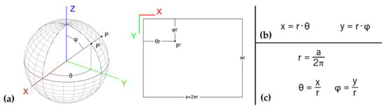
Figure 1.
Relations between spherical coordinates and coordinates on spherical photographs, where is the origin of the polar system, is a point in the 3D space, is the point projection on the sphere, is the horizontal angle, is the vertical angle, and is the radius of the sphere. (a) Graphical representation of the relations between polar coordinates measured by the terrestrial laser scanner and coordinates on the raster image in spherical projection [38], (b) formula which allows for recalculation of polar coordinates onto raster coordinates in spherical projection, and (c) formula that allows for recalculation of x,y raster coordinates in spherical projection onto polar coordinates.
A spherical image for which the raster grey-level value assumes the laser beam reflectance intensity value is used, together with the map of depth (i.e., the distance to the analysed object), for TLS data orientation.
2.2.2. A Virtual Image
Spherical images, as the result of point cloud transformation, are burdened by geometrical deformations. However, it is possible to eliminate existing deformations and to improve the process of searching for tie points, via transformation to a “virtual image” form. For this purpose, the collinearity equation is used [11,17].
In the process of point cloud transformation to the “virtual photograph” form (from 3D to 2D), it is assumed that the projection centre is located at the origin of the instrument coordinate system. The perpendicular to the photographic plane is connected with the assumed scanning angle and the parameter c depends on the focal length of the “virtual image”. The laser beam reflectance intensity value or the colour acquired from an integrated camera is assumed to be the grey-level value. Contrary to the case for spherical images, a map of depth is not generated for the virtual image.
Depending on the assumed constant c of the “virtual camera”, a pixel on an image is defined, which is explicitly connected with the resolution of the utilized images.
2.2.3. An Orthoimage
An orthoimage is generated as a result of photograph processing based on the Digital Surface Model (DSM) in the orthorectification process, when the transformation from the central projection into the orthogonal projection is performed. As a result, deformations caused by distortion, by the influence of the central projection, and by variations in the depth of the analysed object, are limited. The key stage of the generation of orthoimages is a correct interpolation of the DSM [39,40,41].
Thanks to the ordered method of TLS data recording (Section 2), it seems natural to generate the DSM as a regular grid. Moreover, the use of this structure for data recording allows for amendment of blind spots generated as a result of the point cloud filtration. The value of the laser beam reflectance intensity and the distance from the scanner station to the analysed object is assigned to each grid node (recorded in the form of a map of depth).
2.2.4. The TLS Point Cloud in Cartographic Projection
Cartographic transformations are also applied for processing the point cloud to the raster form. In mathematical cartography, the reference surface is assumed to be an ellipsoid or a sphere, as the so-called surface of the original. The term “cartographic projection” is understood as a regular transformation of a flattened rotatable ellipsoid or the transformation of a sphere into a plane [42]. In this paper, only the mathematical notation for projection of a sphere onto a plane is used, which may be described by the following Equations (3) and (4).
Vector equation of a sphere:
The equation of an image of a sphere in a plane:
where are orthogonal coordinates on the sphere surface, are spherical coordinates on the sphere surface, and are orthogonal coordinates on a plane.
Projection regularity condition:
For each point of a sphere the system of inequalities (5) must also be satisfied.
The cylindrical projection relies upon projecting a sphere onto the side of a cylinder, the rotation axis of which corresponds to the straight line, which connects the geographical poles.
Transformation of a sphere onto a plane is expressed by Equation (6).
where is the constant of the cylindrical projection, is the geographical longitude, and is the geographical latitude.
In the cylindrical projections, images of parallels, B = constant, are presented in the form of straight lines parallel to the y-axis of the orthogonal coordinate system. Meridians, L = constant, are projected in the form of straight lines parallel to the x-axis of the coordinate system.
During the terrestrial laser scanning data orientation process, raster images in Mercator cylindrical equal-angle projection were also applied. Conversion of point coordinates to the form of this projection is performed using Equation (7).
where is the radius of a sphere (equal to one unit) and are horizontal and vertical angles, respectively.
In this projection, the grid is an orthogonal network. Images of meridians and parallels are straight lines parallel to respective axes of the planar coordinate system. Poles of the geographic system are projected to infinity. Therefore, this projection is used only within parallel zones, without circumpolar areas [42].
Other cartographic projections have been analysed in detail by Reference [18].
2.2.5. Advantages and Disadvantages of Selected Cartographic Projections
The advantage of using the point cloud in the form of a spherical image is the processing speed for its generation, without the necessity of performing additional interpolation of new pixel values as the process is performed directly on the raw point cloud. However, the disadvantages of this method should be also considered. They include deformations of a generated image, such as the effect of “distortion” and large deformations, which occur for large values of angles, i.e., in the upper and lower parts of the raster. These geometric failures considerably influence the number and the distribution of tie points detected by algorithms applied in digital image processing [12,36,37].
The main advantages of point cloud representation in the form of a “virtual image” include the possibility of applying algorithms that are commonly used for matching images and of eliminating the influence of “distortion”, which occurs in spherical images. The basic disadvantage of this method is caused by the selection of an appropriate constant value for the “virtual camera”. Any change in this parameter directly influences the resolution of the resulting image and makes it necessary to interpolate new pixel values. Additional problems occur when the reference plane is defined, since it requires additional transformations of the XYZ coordinates acquired by the terrestrial laser scanner [11,17].
The advantage of representing the point cloud in the form of an orthoimage is the elimination of the geometric deformations occurring in spherical images. Recording the data in an arranged way simplifies the generation of the DSM in the grid form. Moreover, this method of DSM recording does not require interpolation of new pixel values. The main disadvantage of the method is related to difficulties in detection and interpolation of planes used to generate the DSM. Detailed descriptions and comparisons of different algorithms for detection of planes are presented in publications on computer vision and photogrammetry [43,44,45]
The advantage of using cartographic projections to represent the point cloud is the possibility of considering deformations in the process of raster data generation. The Mercator projection allows for projection of the upper fragments of scans with smaller geometric deformations.
3. Materials and Methods
3.1. Overview of the Approach
The proposed automation of registration is a multi-stage process; it is based on the original software and it consists of (1) data conversion to the raster form, (2) aligning of pairs of raster TLS data for all possible combinations based on SURF and FAST algorithms, (3) the analysis of the quality of relative orientation of processed pairs, and (4) the final bundle adjustment.
The presented TLS data processing is an original approach. As a result of this process decision may be made whether the obtained results meet the assumed accuracy criteria or they are considered as an approximation of the ICP method. For that purpose, the original application, as well as external software tools (LupoScan3D (Pro 2018.2, Lupos3D, Berlin, Germany, 2018), ArcMap 10.2.2 (Esri, Redlands, CA, USA, 2014)) were applied.
In order to perform a complete analysis of the possibilities for applying algorithms for detecting tie points on an intensity raster, the form of the point cloud transformation should be determined to obtain the best results. Verification of the following parameters was required.
- The time of pre-processing of the RAW TLS data.
- The time of detection of characteristic points.
- The percentage of incorrectly detected points and adjusted characteristic points.
- The completeness of data registration
- The number of detected control and check points.
- The orientation accuracy of control and natural and marked check points.
- The distribution of control and check points.
Then, it was possible to assess which method of point cloud representation allowed the highest accuracy to be obtained for TLS data.
The diagram showing research work and experiments performed is presented in Figure 2.
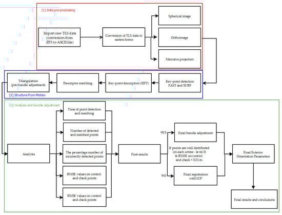
Figure 2.
Diagram of the performed research: Processing and orientation of terrestrial laser scanning data based on the use of raster images in different cartographic projections of the intensity. TLS: Terrestrial Laser Scanning.
Point clouds acquired by Z + F 5003 and Z + F 5006h terrestrial laser scanners were stored in binary form. Binary files, contrary to simple text files, do not have a uniform structure and they cannot be processed directly. Thus, it was decided to use a temporary version of the Software Development Kit (SDK) of the Z + F scanner. Importing and conversion of TLS data were performed by means of the original application based on the SDK tools of the scanner.
The idea of the automatic TLS data registration presented in this paper (according to the diagram presented in Figure 2) consists of the following stages:
- generation of intensity rasters in the spherical projection and orthoimages (with the depth map) using LupoScan and rasters in the Mercator projection and maps of XYZ coordinates in the original application and in ArcMap.
- detection of characteristic points using the SURF (blob) and FAST (point) detectors on point clouds processed to the raster form in the spherical projection, in the Mercator projection and in orthoimages.
- 2.1. generation of pairs of raster using the methods of permutations without repetitions , where: k = 2 (a pair of scans), n - the number of all scans-the spherical projection and the Mercator projection,
- 2.2. generation of pairs of raster using the methods of permutations without repetitions , where: l - the number of planes (the number of walls, the ceiling, and the floor) k = 2 (a pair of scans), n - the number of all scans-orthoimages,
- 2.3. the complete process of calculations was performed for all projections (2.1 and 2.2) using SURF and FAST algorithms.
- description of all detected points by SIFT descriptor,
- matching possible tie points (on pair of rasters) in relation to features with the use of the Brute Force Matching algorithm (Triangulation),
- adjustment of possible characteristic points by means of the pre-bundle adjustment method on the pair of rasters; the iterative process with point filtration (RANSAC method):
- 5.1.
- filtration under the assumptions of three thresholds 0.5m, 0.1 m and 0.01 m.
- 5.2.
- the analysis of the number and distribution of detected tie points,
- 5.3.
- the analysis of values of deviations on points and distributions of points: If points are evenly distributed within the entire scans and the deviation on points <= 0.01 m the detected points are applied during the stage six. Otherwise, the detected points are applied to determine approximate elements of the exterior orientation, considered as the approximation of the ICP method.
- 5.4.
- division of tie points into two groups: Control and check points—the method of division of points considered the division of an image into four parts, ensuring equal distribution of both types of points within the entire object. Their number was analysed in each part; if it was greater than six, every sixth point was considered a check point.
- 5.5.
- determination of approximate elements of the exterior orientation and the analysis of RMSE values on control and check points used in step six.
- Final bundle adjustment for all of the pair of TLS data to defined as the reference scan.
Algorithms for searching and initial matching of tie points were implemented in the original software application, developed in the C++ programming language. For this purpose, the OpenCV library of functions was used, which allowed for reading raster data, searching for characteristic points using the FAST, SURF, etc., algorithms and describing points by means of descriptors of relative matching of features.
The initial filtration of outliers was performed using software tools based on the functions of the Armadillo library [46], utilizing LAPACK algorithms. The analyses of the graphical representations of results were performed using the MATLAB (2016b, MathWorks, Natick, MA, USA, 2016)) application.
Data Pre-Processing
The first stage of raw TLS data processing relies on the import of raw TLS data recorded in the binary form. Thus, it was decided to use a temporary version of the Software Development Kit (SDK) of the Z + F scanner. As a result, it was possible to read TLS data and store it in the ASCII format (a pts file). The number of points was recorded in the Header; the following information was recorded in successive lines: Horizontal and vertical angels, distance, full intensity, and XYZ coordinates of each point. Basing on original (unprocessed) data the full intensity and horizontal and vertical angles (Hz and V) were applied; they were used to generate a spherical image and an orthoimage in the LupoScan application and in the Mercator projection, based on the original application in C++ and ArcMap, applied for generation of raster images.
In order to determine the XYZ coordinates of tie points detected in the intensity raster images in the pixel system, it was necessary to perform data conversion in two ways. In the case of the spherical projection and orthoimages, LupoScan software tools were used, and the process itself relied upon import of a text file containing pixel coordinates to LupoScan and export of the obtained XYZ coordinates to a text file. Raster images in XYZ coordinates were determined using ArcGIS software and its Model Builder functionality (the functional diagram is presented in Figure 3).
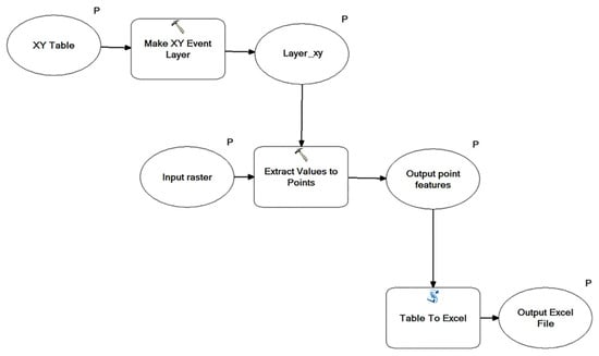
Figure 3.
The functional diagram for the determination of XYZ coordinates based on pixel coordinates for raster images in the Mercator projection.
3.2. Characteristics of Raw Data and Selected Test Sites
In order to verify the assumed idea of selection of the cartographic conversion of TLS data in the automated data orientation process, four test sites were selected (two decorated historical chambers at the Museum of King Jan III’s Palace at Wilanów) and the office room and empty shop at the shopping mall characterized by a not diversified structure and the surface geometry. Selected test sites necessary for verification of the effectiveness of point detection algorithms and an appropriate representation of a point cloud (raster images in the spherical projection, the Mercator projection, and as orthoimages) were characterized by varied dimensions, texture, adornments, and geometric complexity level. TLS data were acquired by two scanners: Z + F 5003 and Z + F 5006h. Additionally, in order to verify the assumed idea of data registration, two scanning variants were selected in each test site: (scenario A) close scanner stations where the same fragments of the surface are measured under similar angles and (scenario B) fragments of the surface measured under different angles from different distances and heights of the TLS positions. A scan located in the centre of and analysed chamber, having the highest coverage with remaining scans, was chosen as a reference scan. The process of manual selection of the reference scan was performed at the first stage of data processing.
In order to perform an independent quality assessment, marked control points were distributed on three (out of four) test sites; they were measured using the tacheometric method.
Test site I: “The Queen’s Bedroom”-Museum of King Jan III’s Palace at Wilanów
Test site I was characterized by geometric complexity in the form of rich ornaments, bas-reliefs and facets. Moreover, there were mirrors in golden frames, and they were decorative fireplaces, and fabrics, etc., hanging on the walls (Figure 4).
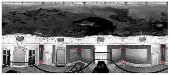
Figure 4.
The point cloud in the spherical projection of test site I: “The Queen’s Bedroom” with marked points (red circles).
Measurements were performed using the phase scanner Z+F 5003 with a scanning resolution of 3.2 mm/10 m. Figure 5a presents the distribution of scanner positions and the scanning distances. Five out of six scans were acquired with the selected fragment of a chamber (the incomplete extent).
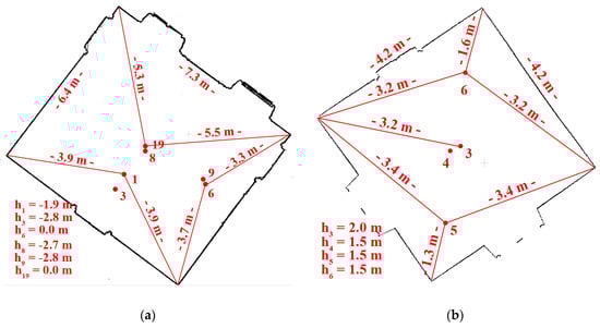
Figure 5.
The floodplain with marked TLS scanner position with distances to the nearest walls for: (a) test site I: “The Queen’s Bedroom” and (b) site II: “The Chamber with a Parrot”. In the figures, the high of of each TLS station, related to the reference scan was presented. The h values are related to the high of the reference scan.
The nineteenth scan (acquired with the full angular resolution) was applied as the reference scan. Sixteen marked points were distributed over the test site (considered as check points in further analyses), which were used for TLS data orientation.
Test site II: “The Chamber with a Parrot”-Museum of King Jan III’s Palace at Wilanów
The characteristic features of test site II were the small number of ornaments and the lack of bas-reliefs, facets or fabrics on the walls. In this case, the walls were painted with patterns, which imitated spatial effects (Figure 6). An inventory of test site II was performed using the Z + F 5006h scanner (the newer generation), which was used to acquire four scans with a horizontal extent of 360˚ and a scanning resolution of 3.2 mm/10 m. Figure 5b presents the distribution of scanner positions and scanning distances, where the first scan was considered as the reference scan. Due to the prohibition to located marked points on historical surfaces, automatically detected points defined as check points, were used for the accuracy analysis.
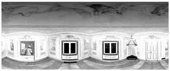
Figure 6.
The point cloud in the spherical projection of test site II: “The Chamber with a Parrot” without marked points.
Test site III: “The office room”
Test site III is an office room, with a narrow lobby, where eight scans were acquired with a horizontal extent of 360° and a scanning resolution of 6.2 mm/10 m. On the analysed test site, walls were smooth, without the texture; lamps and power wires were located on the ceiling and the floor was covered with the dark carpet (Figure 7). Figure 8a presents the distribution of scanner stations and scanning distances.
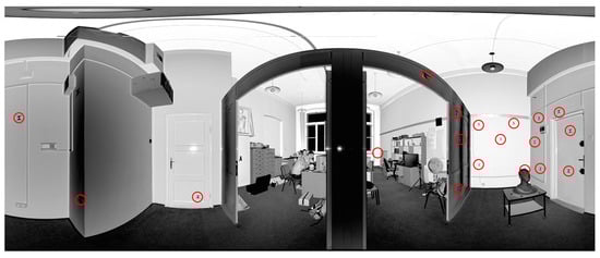
Figure 7.
The example of the point cloud in the spherical projection of test site III: “The office room” with marked check points (red circles).
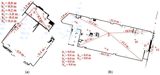
Figure 8.
The floodplain with marked TLS scanner position with distances to the nearest walls for: (a) test site III: “The office room” and (b) test site IV: “Empty shop (shopping mall)”. On figures, the high of each TLS station, related to the reference scan was presented. The h values are related to the high of the reference scan.
Scan six was used as the reference scan and 19 marked points were distributed over the test site (considered as check points in further analyses) which were used for TLS data orientation.
Test site IV: “Empty shop (shopping mall)”
Test site IV is an empty shop room where 7 scans were acquired with a horizontal extent of 360° and a scanning resolution of 12 mm/10 m. The walls of the room were smooth, without texture. Lamps, electric wires and an air-conditioning system were located on the ceiling; the floor was made of concrete (Figure 9). Figure 8b presents the distribution of scanner stations and scanning distances.
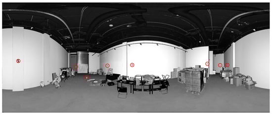
Figure 9.
The example of the point cloud in the spherical projection of test site IV: “Empty shop (shopping mall)” with marked check points (red circles).
Scan eight was used as the reference scan and eight marked points were distributed over the test site (considered as check points in further analyses), which were used for TLS data orientation.
4. Results
4.1. Time of TLS Data Conversion
Table 1 presents the average time of TLS data conversion for particular cartographic projections and test site in minutes and seconds. For planes detection, the Hough 2D method were used [44].

Table 1.
The pre-processing data time.
It can be seen from Table 1 that the shortest time for data conversion into the raster form is obtained in the case of the spherical images and the longest time in the case of the orthoimage (Test site III). The time of processing TLS data to the orthoimages depends on the number of detected planes and it is an influence on the complexity of the process of computations [44].
4.2. Time for Tie Points Detection and Matching
The first test was an analysis of the average time for detection and matching of characteristic points on all pairs of raster images in the various projections for both test sites (Table 2) in minutes and seconds.
Table 2.
Time for detection and matching of characteristic points for particular projections of point clouds, for test sites I and II (both scenarios).
It can be seen from Table 2 that the shortest time for searching and matching of characteristic points for all algorithms is obtained in the case of both test sites for representation of the point cloud in the form of an orthoimage; longer times are obtained for the Mercator projection and the spherical image, respectively. Regarding computation times for all analysed cases, the shortest time is obtained when the FAST detector is used.
4.3. The Number of Points Detected on Raster Images
The following coefficients were verified for the requirements of the assessment of the number of detected points for all pairs of raster images (from all projections): The average, the maximum and the minimum number of detected and matched key points (characteristic points) (Table 3) and the percentage of incorrectly detected and matched key points (characteristic points) (Table 4). Statistical data was developed with the use of the original application in Matlab software. The statistics presented in Table 3 show the detector effectiveness (statistics of numbers of detected points) on the different test sites in each of the three cartographic transformations.
Table 3.
Statistics of number of detected and matched keypoints for particular projections of point clouds for all test sites (both scenarios).
Table 4.
The percentage number of incorrectly detected and matched keypoints for particular projections of point clouds for all test sites (both scenarios).
The analyses performed for test site I show that, on average, the minimum and maximum numbers of points (for all pairs of scans) were detected using FAST and SURF detectors, respectively, for scans in the spherical projection, using FAST and SURF detectors in the case of orthoimages and using SURF and FAST detectors for the Mercator projection. The largest number of corresponding points was obtained for the SURF detector with the use of spherical images.
Based on the analysis of data acquired from test site II, it may be stated that the highest numbers of tie points were detected using the FAST detector for raster images in the Mercator projection, orthoimages and spherical images. Using the SURF detector, the largest maximum numbers of tie points were detected for raster images in the spherical and Mercator projections (about three times more than for orthoimages). Rasters in the Mercator projection were characterized by the largest mean numbers of detected characteristic points, with a value three times larger than for other projections. Due to the lack of texture and characteristic geometrical shapes for test sites III and IV, the algorithms detected and matched a considerably smaller number of tie points. In the case of Test site IV (a long and narrow shop in the shopping mall), the sufficient number of points was obtained only for raster images in the spherical projection and for orthoimages. Resuming, the greatest number of tie points the greatest number of tie points was detected for Test site II. While the analysed object was not geometrically complicated and had the smooth ceiling and oak parquet, due to painting on the walls tie points were best detected and matched by detectors. In the case when the office or industrial objects are analysed (having poor texture and low geometric diversification) it is recommended to use a FAST detector and raster images in spherical projection and orthoimages.
At the first stage of tie point’s detection, the process of tie matching points in pairs consisted of the analysis of the descriptor, which was based on the reflection intensity of the laser beam. Due to the fact that analysed scans were acquired under different angles and from different distances from surfaces being measured, the laser beam reflectance intensity was not uniform and it was characterised by the high diversification of tonal values. For such raster images, the algorithms developed for image matching did not always operate correctly and they required another approach to filtration of possible tie points. Another factor that influenced incorrect detection and matching of tie points included geometric deformations ("distortion"), which occurred in raster images in the spherical projection and in the Mercator projection. Therefore the RANSAC algorithm with parameters presented in Figure 2 was applied for initial detection of corresponding tie points. As a result of filtration, the percentage of incorrectly matched points was determined using the descriptor analysis only and then their percentage in the total number of detected and matched points was also determined (Table 4).
4.4. Evaluation of Correctness of Automatic Matching Pairs of Scans
In order to determine the effectiveness of connection of scans, the correctness and completeness of orientation of all pairs of scans were analysed for investigated test sites. The following assumptions were made for the needs of evaluation: Full-registration, which did not require final registration by means of another method (deviation on points ≤0.01 m and correct distribution of tie points), semi-registration, which is the approximate registration (approximate exterior parameters considered as initial parameters for ICP) and no-registration, which does not allow it to perform the process of orientation. In order to present the extent of performed investigations and the number of combinations of connection of scans in pairs for all test sites and projections, results of connection of scans are presented in Table 5, Table 6, Table 7 and Table 8. The green colour marks correct matching (full-registration), the initial orientation that requires the final registration using the ICP method is marked in orange, and the red colour means lack of matching; the "x" symbol means no connection of scans on pairs due to a lack of mutual overlap.
Table 5.
The correctness of automated connecting of scans for Test Site I (both scenarios): Green, correct matching (full-registration), orange, preliminary orientation requiring the final registration using the ICP method, red, no matching, and “x”-means not connection for scans (no overlap).
Table 6.
The correctness of automated connecting of scans for Test Site II (both scenarios): Green, correct matching (full-registration), orange, preliminary orientation requiring the final registration using the ICP method, red, no matching, and "x", means not connection for scans (no overlap).
Table 7.
The correctness of automated connecting of scans for Test Site III (both scenarios): Green, correct matching (full-registration), orange-preliminary orientation requiring the final registration using the ICP method, red, no matching, and "x", means no connection for scans (no overlap).
Table 8.
The correctness of automated connecting of scans for Test Site IV (both scenarios): Green, correct matching (full-registration), orange, preliminary orientation requiring the final registration using the ICP method, red, no matching, and "x", means not a connection for scans (no overlap).
Basing on results listed in Table 5 it may be stated that most of pairs were correctly matched.
All pairs of scans were correctly matched and oriented using the FAST and SURF detectors.
In the case of Test site III (and office space with a narrow lobby) higher diversification of correct matching of particular pairs of scans may be observed. All pairs of scans were correctly matched with an orthoimage using the FAST detector. When the connection of pairs of scans in the spherical projection is analysed, it is recommended to commonly apply two detectors (FAST and SURF). In the case of the Mercator projection, it is not recommended to apply the FAST detector.
Performed tests proved that the worst results were obtained for Test site IV (an empty shop in the shopping mall) with smooth walls and dark surfaces of the air-conditioning system. In the case of such rooms, an individual approach to scanning and the use of raster images is required. Performed tests proved incorrect operation of applied algorithms although the scans were acquired with the high overlap. The registered intensity and the point cloud density did not allow detection of the sufficient number of correctly distributed tie points. Therefore, it may be concluded that the processing of such a point cloud to the raster form in proposed cartographic projections does not guarantee the correctness and completeness of the data orientation process with the use of the SURF and FAST algorithms. The authors plan to perform the analysis of a selection of other detectors for such objects.
4.5. Accuracy Analysis on Natural Control Points
Table 9 presents statistics of the linear RMSE error values on control points detected in pairs of raster images for both scenarios by means of the SURF and FAST detectors in the spherical projection, in the Mercator projection and in orthoimages. In Table 9, only the maximum, minimum, and average values of RMSE for all pair of scans were presented. The accuracy analysis was separately presented for X, Y, and Z components in Table S1.
Table 9.
The statistics of the RMSE values on natural control points for all test sites (both scenarios).
Based on the results presented in Table 9, it may be noticed that the orientation accuracy on natural control points is similar for Test site I (3.5–4.0 mm); for Test site II it is considerably better for raster images in the spherical projection, it is about two times better. For Test site III, which is characterised by the poorer texture the lower orientation accuracy was obtained, in the range of 5–6 mm; it is similar for all cartographic projections. In the case of Test site IV, where the scanning resolution equalled to 1.2 mm/10 m and the orientation process has not been successfully completed for particular pairs, it was possible to estimate the orientation accuracy only for the spherical projection for which the orientation error equalled to 9.0 mm for the SURF algorithm and 34.2 mm for the FAST algorithm.
4.6. Accuracy Analysis on Natural and Marked Check Points
For the needs of an independent evaluation of the accuracy of the TLS data orientation process the accuracy analysis was performed on (natural and marked) check points, which were not participating in the data adjustment, and therefore, reliable analysis results could be obtained. Table 10 and Table 11 present the statistical values of linear RMSE for two scenarios: (scenario A) close scanner stations where the same fragments of the surface are measured under similar angles and (scenario B) fragments of the surface measured under different angles from different distances and heights of the TLS positions. The accuracy analysis was separately presented for X, Y, and Z components in Table S2. Any marked points were distributed in Test site II and there was no scenario A for Test site IV.
Table 10.
The statistics of the RMSE values on natural and marked check points for all test sites (scenario A).
Table 11.
The statistics of the RMSE values on natural and marked check points for all test sites (scenario B).
When results from Table 10 are analysed, it turns out that better accuracy was obtained for natural check points. This results from the fact that it is the Root Mean Square Error, and the number of natural detected points was considerably higher and this influenced the averaging of results.
In scenario B (Table 11) the error values are comparable with results presented in Table 10, this proves the methodological correctness of the TLS data registration process in cartographical projections. Another issue is connected with Test site IV, which was scanned with the lower resolution and worse geometry of scanner stations. This influenced the entire process of data processing and orientation.
5. Discussion
The proposed automatic TLS data registration approach based on three main steps: (1) TLS data conversion into the raster form based on the cartographical transformation (spherical image, orthoimage, and Mercator projection); (2) detect tie points with SUIRF and FAST algorithm, and (3) exterior orientation parameters estimation in iterative bundle adjustment process.
The conventional, target-based, method of TLS point cloud registration consists of measurements of marked points, which are evenly distributed on an analysed object. Dedicated software applications are usually applied which allow measuring points in raster images in the spherical projection. In the proposed method the authors utilise functions of the SDK library allowing the acquisition of RAW data without the necessity to use external software. Comparing the time of raster generation using the proposed method and the original software it may be noticed that the proposed method is time-consuming, but it allows for preparation of RAW data, to generate raster images in the selected cartographic projection in order to automatically detect tie points, using detectors, such as FAST and SURF. Selection of those detectors resulted from preliminary tests, performed by the authors for other objects, such an open landscape [12] or historical interiors [37]. Differences in the approach relied upon the use of TLS data directly processed with the Z + F LaserControl application (they were not the RAW data), the scanner positions were similar to scenario A, and the castle ruins were the measured object. Tests performed in Reference [37] proved the correctness of operations of the SIFT detector. Due to time-consuming automatic searching for planes for orthoimages, it was decided to apply the Mercator projection. Earlier tests proved that, using spherical raster images, it is not possible to detect tie points on the ceiling.
Due to the fact that the intensity of laser beam reflectance differs and it depends on the distance and the scanning angle, the same areas are characterised by the different intensity in different raster images. This influences the correctness and the number of initial tie points. Therefore, it is also necessary to perform the proposed initial filtration and orientation of tie points with the use of the RANSAC algorithm in the TLS registration process.
When results presented in Table 3 and Table 4 are analysed, it may be noticed that in the case of test sites of historical objects (Site I and II), the FAST, as well as the SURF algorithms detected the high number of possible tie points which quality turned to be low. Thus, the great number of tie points does not always prove the better process of point matching. This was also proved by the number of rejected points. In general, it may be stated that the best results were obtained for point clouds acquired with the limited angular resolution in the Mercator projection (Test site I). In the case of the full angular resolution, the best results were obtained for orthoimages (Test site II). In the case of Test sites III and IV, which were walls were smooth without architectural decorations, the number of detected tie points were considerably smaller. Paradoxically, despite the smaller number of points, the majority of them were not rejected in the data filtration process; this proves the correct matching of descriptors. For such room, it is recommended to use the spherical projection. The SURF and FAST detectors allow detecting the similar number of correct tie points.
To perform the TLS data registration methodology based on raster images, the orientation of the same scans was performed using the target-based registration method in Z + F LaserControl software. It was performed on the same test sites where marked checked points were located (Table 12).
Table 12.
Comparison of results of TLS reatser images orientation and the target-based registration method.
When results presented in Table 12 are analysed, it may be noticed that the proposed method allow obtaining better accuracy for all cartographic projections for historical objects which are characterised by the high number of architectural details and diversified texture. In the case of Test site III (office room) the results are worse than in the case of utilisation of the target-based method, however, the error values allow to obtain the correct orientation when more points are used. In the case of Test site IV, the results obtained by means of the proposed method should be considered as an approximation of the orientation performed using the ICP method.
Two different test sites were selected for the analysis of the distribution of natural control and check points. Appendix Figure A1, Figure A2, Figure A3 and Figure A4 presents the best and the worst distribution of natural check and control points for particular scanner stations on test sites I and III.
When the distribution of points presented in Figure A1 (Test site I) is analysed, it may be noticed that the highest number of control and check points was detected for the orthoimage and the FAST detector. For remaining cartographic projections the number and distribution of control and check points also guarantee the correct implementation of the orientation process. When results presented in Figure A2 are analysed, it may be noticed that the worst distribution and the smallest number of points were obtained for the Mercator projection and for the SURF detector. In the case of Test site III (Figure A3), which is an office room, the best distribution and the best number of points were obtained for spherical projections and for the Mercator projection for both detectors (FAST and SURF). However, when the distribution of points from the orthoimage is analysed, they may also be considered correct. When results presented in Figure A4 are analysed, the smallest number of points and the worst distribution were obtained for points detected in raster images in the Mercator projection. To summarize, an important aspect related to data orientation is not only the number of tie points but also the distribution of points which influences on the quality of TLS data registration.
It is not possible to propose one, universal form of point cloud representation allowing the above requirements to be met. Therefore, a priori knowledge concerning the positions of the scanner stations is required, allowing for selection of the optimum representation of a point cloud. It is necessary to separately consider two cases, i.e., closely located scanner stations where the same fragments of an object are measured under similar angles (a situation which does not result in a high influence of “distortion” in spherical images) and scanner stations from which fragments of an object are measured under different angles and from different distances.
When the registration of point clouds acquired from close scanner stations is performed, it is recommended to use raster images in the spherical or the Mercator projections. Selection of a particular projection is directly connected with the position of the scanner station. If the instrument is placed lower, (i.e., closer to the floor) it is reasonable to use raster images in the Mercator projection, though not when the scanner is located closer to the ceiling, since data from fragments of a cloud projected from the ceiling are not lost. The analysis of the distribution of tie points shows that for close scanner stations, the best and most even distribution of control and check points was obtained for raster images in the Mercator projection, for orthoimages and for spherical images, respectively.
In the case where point clouds are acquired from stations for which fragments of an analysed object are measured under considerably different angles and from a different distance, it is recommended to use orthoimages. The use of other forms of point cloud representation influences the presence of “distortion”, which is directly connected with difficulties in explicit identification of tie points when using any algorithm for detecting characteristic points. When RMSE error values are analysed for points detected both on fragments and on entire scanned areas, it may be noticed that the difference between them is twice as high. Therefore, it is recommended to acquire scans at the maximum angular resolution.
In the summary, it should be stressed that the proposed method is recommended for historical rooms where it is not possible to place marked points on the object surface. In the case of complex objects, it is possible to process RAW data in such a way that the automatic and more accurate orientation of scans could be obtained. It also allows for selecting the determined cartographic projection that influences the better detection of evenly distributed tie points. Compared to the conventional, target-based approach, the number of detected control and check points is considerably bigger; this influences the registration accuracy. The authors have utilized the proposed method for measurements performed at the Museum of King Jan III’s Palace at Wilanów and in the Royal Castle in Warszawa.
6. Conclusions
The analyses show that the first two stages, i.e., selection of an appropriate method of TLS point cloud conversion to the raster form and selection of an appropriate algorithm, considerably influence the completeness of the entire process and the accuracy of data orientation.
In the case of the orientation of scans processed into the raster forms, angles under which analysed surfaces are measured should be considered; this is reflected in the quality and accuracy of finding tie points. If scanner stations are located close to one another, similar deformations in the form of “distortion” appear in raster images in the spherical and Mercator projections. When the blob and the corner detection algorithms are used, detection of characteristic points should not highly influence their number and distribution. If scans from highly diversified positions of the scanner stations are oriented, the issue concerning the unequal influence of “distortion” in raster images in the spherical and Mercator projection appears. This influences the explicit identification of the same characteristic points and their correct distribution. Therefore, it is recommended to convert the point cloud to the orthoimage form. As a result of the elimination of the discussed deformations, it is possible to achieve high accuracies of data orientation and correct locations of tie points, since detectors have no problems with their explicit identification.
Before the TLS data orientation process starts, it is recommended to divide point clouds according to the method of conversion (to the raster form in the spherical/Mercator projection or to orthoimages) and the use of point detectors or blob algorithms to detect points.
Supplementary Materials
The following are available online at http://www.mdpi.com/2076-3417/9/3/509/s1, Table S1: Quality assessment on natural control points, Table S2. Quality assessment on natural and check points.
Author Contributions
J.M. designed the main idea and manuscript, designed the proposed methods and algorithms, wrote the manuscript and performed experiments, D.Z. discussed the main idea; co-wrote the Results and Discussion.
Acknowledgments
The authors would like to thank the Museum of King Jan III’s Palace in Wilanów for cooperation.
Conflicts of Interest
The authors declare no conflict of interest.
Appendix A Analysis of the Distribution of Tie Control and Check Points
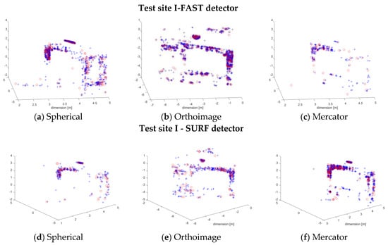
Figure A1.
Distribution of points used in the TLS data orientation process for the pair of scans for the scanner stations for test sites I: “The Queen’s Bedroom”-the best distribution of the control (blue) and check points (red). Points detected by FAST (a–c) and SURF (d–f) detectors on raster images: (a/d) in the spherical projections, (b/e) in the orthoimage and (c/f) in the Mercator projection.
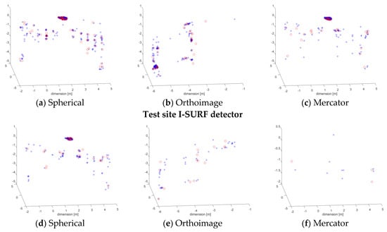
Figure A2.
Distribution of points used in the TLS data orientation process for the pair of scans for the scanner stations for test sites I: “The Queen’s Bedroom”-the worst distribution of the control (blue) and check points (red). Points detected by FAST (a–c) and SURF (d–f) detectors on raster images: (a/d) in the spherical projections, (b/e) in the orthoimage and (c/f) in the Mercator projection.
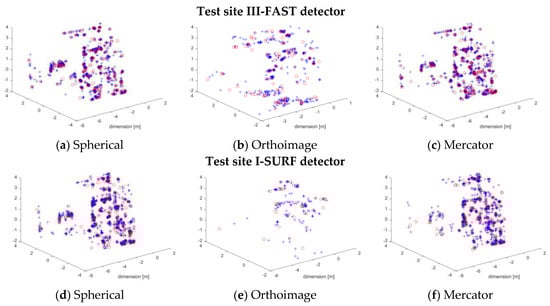
Figure A3.
Distribution of points used in the TLS data orientation process for the pair of scans for the scanner stations for test sites III: “The office room”-the best distribution of the control (blue) and check points (red). Points detected by FAST (a–c) and SURF (d–f) detectors on raster images: (a/d) in the spherical projections, (b/e) in the orthoimage and (c/f) in the Mercator projection.
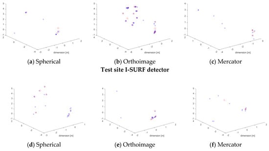
Figure A4.
Distribution of points used in the TLS data orientation process for the pair of scans for the scanner stations for test sites III: “The office room”-the worst distribution of the control (blue) and check points (red). Points detected by FAST (a–c) and SURF (d–f) detectors on raster images: (a/d) in the spherical projections, (b/e) in the orthoimage and (c/f) in the Mercator projection.
References
- Remondino, F.; El-Hakim, S. Image-based 3D Modelling: A Review. Photogramm. Rec. 2006, 21, 269–291. [Google Scholar] [CrossRef]
- Balzani, M.; Pellegrinelli, A.; Perfetti, N.; Uccelli, F. A terrestrial 3D laser scanner: Accuracy tests. In Proceedings of the 18th Int. Symp. CIPA 2001- Surveying and Documentation of Historic Buildings, Monuments, Sites - Traditional and Modern Methods, Potsdam, Germany, 18–21 September 2001. [Google Scholar]
- Byrne, D. ContextCapture ® Software to Automaticly Generated Detailed 3D Models from Photographss. Product Data Sheet, 2016.
- Markiewicz, J.; Podlasiak, P.; Kowalczyk, M.; Zawieska, D. The new approach to camera calibration-GCPs or TLS Data? In International Archives of the Photogrammetry, Remote Sensing and Spatial Information Sciences - ISPRS Archives; 2016; Volume 41. [Google Scholar]
- Paris, C.; Kelbe, D.; Van Aardt, J.; Bruzzone, L. A Novel Automatic Method for the Fusion of ALS and TLS LiDAR Data for Robust Assessment of Tree Crown Structure. IEEE Trans. Geosci. Remote Sens. 2017, 55, 3679–3693. [Google Scholar] [CrossRef]
- Zhang, R.; Li, H.; Liu, L.; Wu, M. A G-Super4PCS Registration Method for Photogrammetric and TLS Data in Geology. ISPRS Int. J. Geo-Inf. 2017, 6, 129. [Google Scholar] [CrossRef]
- Alba, M.; Barazzetti, L.; Scaioni, M.; Remondino, F. Automatic Registration of Multiple Laser Scans Using Panoramic Rgb and Intensity Images. ISPRS Int. Arch. Photogramm. Remote Sens. Spat. Inf. Sci. 2012, 49–54. [Google Scholar] [CrossRef]
- Wang, Z.; Claus, B. Point based registration of terrestrial laser data using intensity and geometry features. IAPRS SIS 2008, 583–589. [Google Scholar]
- Urban, S.; Weinmann, M. Finding a Good Feature Detector-Descriptor Combination for the 2D Keypoint-Based Registration of Tls Point Clouds. ISPRS Ann. Photogramm. Remote Sens. Spat. Inf. Sci. 2015, II-3/W5, 121–128. [Google Scholar] [CrossRef]
- Theiler, P.W.; Schindler, K. Automatic Registration of Terrestrial Laser Scanner Point Clouds Using Natural Planar Surfaces. In Proceedings of the XII ISPRS Congress, Melbourne, Australia, 25 September–1 October 2005. [Google Scholar]
- Moussa, W.; Abdel-Wahab, M.; Fritsch, D. an Automatic Procedure for Combining Digital Images and Laser Scanner Data. ISPRS Int. Arch. Photogramm. Remote Sens. Spat. Inf. Sci. 2012, XXXIX-B5, 229–234. [Google Scholar] [CrossRef]
- Markiewicz, J. The use of computer vision algorithms for automatic orientation of terrestrial laser scanning data. ISPRS Int. Arch. Photogramm. Remote Sens. Spat. Inf. Sci. 2016. [Google Scholar] [CrossRef]
- Forssén, P.E. Maximally stable colour regions for recognition and matching. Proc. IEEE Comput. Soc. Conf. Comput. Vis. Pattern Recognit. 2007. [Google Scholar] [CrossRef]
- Agisoft PhotoScan. Available online: http://www.agisoft.com/ (accessed on 31 January 2019).
- Pix4D. Available online: https://pix4d.com/ (accessed on 31 January 2019).
- VFleat. Available online: http://www.vlfeat.org/ (accessed on 31 January 2019).
- Moussa, W. Integration of Digital Photogrammetry and Laser Scanning for Heritage Documentation. Dotctoral Thesis, University of Stuttgart, Stuttgart, Germany, 28 February 2014. [Google Scholar]
- Houshiar, H.; Borrmann, D.; Elseberg, J.; Nüchter, A. Panorama based point cloud reduction and registration. In Proceedings of the 2013 16th International Conference on Advanced Robotics (ICAR), Montevideo, Uruguay, 25–29 November 2013. [Google Scholar] [CrossRef]
- Cheng, L.; Chen, S.; Liu, X.; Xu, H.; Wu, Y.; Li, M.; Chen, Y. Registration of laser scanning point clouds: A review. Sensors 2018, 18. [Google Scholar] [CrossRef]
- Lichti, D.; Pfeifer, N. Introduction to Terrestrial Laser Scanning. 2008, 12219. [Google Scholar]
- Vosselman, G.; Maas, H.-G. Airborne and Terrestrial Laser Scanning. Whittles Publshing: Scotland, UK, 2010; ISBN 978190445876. [Google Scholar]
- Luhmann, T.; Robson, S.; Kyle, S.; Boehm, J. Close-Range Photogrammetry and 3D Imaging, 2nd ed.; Walter De Gruyter: Boston, MA, USA, 2013; ISBN 9783110302783. [Google Scholar]
- Liu, Y. Automatic registration of overlapping 3D point clouds using closest points. Image Vis. Comput. 2006, 24, 762–781. [Google Scholar] [CrossRef]
- Nuchter, A.; Lingemann, K.; Hertzberg, J. 6D SLAM-3D Mapping Outdoor Environments. J. Field Robot. 2007, 24, 699–722. [Google Scholar] [CrossRef]
- Durrant-Whyte, H.; Bailey, T. Simultaneous localization and mapping: Part I. IEEE Robot. Autom. Mag. 2006, 13, 99–108. [Google Scholar] [CrossRef]
- Sprickerhof, J.; Nüchter, A.; Lingemann, K.; Hertzberg, J. An Explicit Loop Closing Technique for 6D SLAM. In Proceedings of the 4th European Conference on Mobile Robots, Mlini/Dubrovnik, Croatia, 23–25 September 2009; pp. 229–234. [Google Scholar]
- Morgan, J.A.; Brogan, D.J. How to VisualSFM 2016. Available online: https://d32ogoqmya1dw8.cloudfront.net/files/getsi/teaching_materials/high-rez-topo/visual_sfm_tutorial.pdf (accessed on 31 January 2019).
- Bay, H.; Ess, A. Speeded-Up Robust Features (SURF). Comput. Vis. Image Underst. 2008, 110, 346–359. [Google Scholar] [CrossRef]
- Bay, H.; Tuytelaars, T.; Van Gool, L. SURF: Speeded up robust features. Lect. Notes Comput. Sci. 2006, 404–417. [Google Scholar] [CrossRef]
- Lowe, D.G. Object recognition from local scale-invariant features. In Proceedings of the Seventh IEEE International Conference on Computer Vision, Kerkyra, Greece, 20–27 September 1999; Volume 2, pp. 1150–1157. [Google Scholar] [CrossRef]
- Lowe, D.G. Distinctive image features from scale-invariant keypoints. Int. J. Comput. Vis. 2004, 60, 91–110. [Google Scholar] [CrossRef]
- Rosten, E.; Drummond, T. Machine Learning for High Speed Corner Detection. In Computer Vision—ECCV 2006; Springer: Berlin/Heidelberg, Germany, 2006; Volume 1, pp. 430–443. [Google Scholar] [CrossRef]
- Brown, M.; Lowe, D.G. Invariant Features from Interest Point Groups. Br. Mach. Vis. Conf. 2002, 656–665. [Google Scholar]
- OpenCV. Available online: http://opencv.org/ (accessed on 31 January 2019).
- Barnea, S.; Filin, S. Extraction of objects from terrestrial laser scans by integrating geometry image and intensity data with demonstration on trees. Remote Sens. 2012, 4, 88–110. [Google Scholar] [CrossRef]
- Markiewicz, J.; Kajdewicz, I.; Zawieska, D. The analysis of selected orientation methods of architectural objects’ scans. Proc. SPIE 2015, 9528, 952805. [Google Scholar] [CrossRef]
- Markiewicz, J.S. The example of using intensity orthoimages in tls data registration—A case study. ISPRS Int. Arch. Photogramm. Remote Sens. Spat. Inf. Sci. 2017. [Google Scholar] [CrossRef]
- Fangi, G. The Multi-image spherical Panoramas as a tool for Architectural Survey. In Proceedings of the XXI International CIPA Symposium, Atene, Greece, 1–6 October 2007; ISBN 0256--1840. [Google Scholar]
- Georgopoulos, A.; Tsakiri, M. Large scale orthophotography using DTM from terrestrial laser scanning. Int. Arch. Photogramm. Remote Sens. 2004, 35, 467–472. [Google Scholar]
- Prouff, E.; Rivain, M. Theoretical and practical aspects of mutual. Appl. Cryptogr. Netw. Secur. 2009, 2, 145–154. [Google Scholar]
- Chiabrando, F.; Donadio, E.; Rinaudo, F. SfM for orthophoto generation: Awinning approach for cultural heritage knowledge. ISPRS Int. Arch. Photogramm. Remote Sens. Spat. Inf. Sci. 2015, 40, 91–98. [Google Scholar] [CrossRef]
- Pędzich, P. Podstawy odwzorowań kartograficznych z aplikacjami komputerowymi; Oficyna Wydawnicza Politechniki Warszawskiej: Warsaw, Poland, 2014. [Google Scholar]
- Deschaud, J.; Goulette, F. A Fast and Accurate Plane Detection Algorithm for Large Noisy Point Clouds Using Filtered Normals and Voxel Growing. In Proceedings of the 3Dpvt, Paris, France, 17–20 May 2010; pp. 1–9. [Google Scholar]
- Markiewicz, J.S.; Podlasiak, P.; Zawieska, D. A new approach to the generation of orthoimages of cultural heritage objects-integrating TLS and image data. Remote Sens. 2015, 7. [Google Scholar] [CrossRef]
- Holz, D.; Behnke, S. Approximate triangulation and region growing for efficient segmentation and smoothing of range images. Robot. Auton. Syst. 2014, 62, 1282–1293. [Google Scholar] [CrossRef]
- Library, A. Available online: http://arma.sourceforge.net/ (accessed on 31 January 2019).
© 2019 by the authors. Licensee MDPI, Basel, Switzerland. This article is an open access article distributed under the terms and conditions of the Creative Commons Attribution (CC BY) license (http://creativecommons.org/licenses/by/4.0/).