Evaluation of Clustering Methods in Compression of Topological Models and Visual Place Recognition Using Global Appearance Descriptors

Abstract

This paper presents an extended study about the compression of topological models of indoor environments. The performance of two clustering methods is tested in order to know their utility both to build a model of the environment and to solve the localization task. Omnidirectional images are used to create the compact model, as well as to estimate the robot position within the environment. These images are characterized through global appearance descriptors, since they constitute a straightforward mechanism to build a compact model and estimate the robot position. To evaluate the goodness of the proposed clustering algorithms, several datasets are considered. They are composed of either panoramic or omnidirectional images captured in several environments, under real operating conditions. The results confirm that compression of visual information contributes to a more efficient localization process through saving computation time and keeping a relatively good accuracy.

1. Introduction

The presence of mobile robots in many kinds of environments has increased substantially during the past few years. Robots need a high degree of autonomy to develop their tasks. In the case of autonomous mobile robots, this means that they must be able to localize themselves and to navigate through environments that are a priori unknown. Hence, the robot will have to carry out the mapping task, which consists of obtaining information from the environment and creating a model. Once this task is done, the robot will be able to address the localization task, i.e., estimating its position within the environment with respect to a specific reference system.

Vision sensors have been widely used for mapping, navigation, and localization purposes. According to the number of cameras and the field of view, different configurations have been proposed. Some authors (such as Okuyama et al. [1]) have used monocular configurations. Others proposed stereo cameras by using binocular (such as Yong-Guo et al. [2] or Gwinner et al. [3]) or even trinocular systems (such as Jia et al. [4]).

Despite stereo cameras permitting measuring depth from the images, these systems present a limitation related to their field of view. In order to obtain complete information from the environment, several images must be captured. In this respect, omnidirectional cameras constitute a good alternative. They can provide a big amount of information with a field of view of 360 deg. around them, and their cost is relatively low in comparison with other kinds of sensors. Furthermore, omnidirectional vision systems present further advantages. For instance, the features in the images are more stable (because they stay longer as the robot moves), and they permit estimating both the position and the orientation of the robot. Omnidirectional cameras have been successfully used by different authors for mapping and localization [5,6,7,8,9]. A wide study was carried out by Payá et al. [10], who introduced a state-of-the-art of the most relevant mapping and localization algorithms developed with omnidirectional visual information. An example of a mobile robot that has an omnidirectional camera mounted on it is shown in Figure 1a, and an example of an omnidirectional image is shown in Figure 1b.

In the related literature, two main frameworks have been proposed in order to carry out the mapping task: the metric maps, which represent the environment with geometric accuracy; and the topological maps, which describe the environment as a graph containing a set of locations with the related links among them. Regarding the second option, some authors have proposed to arrange the information in the map hierarchically, into a set of layers. The way a robot solves the localization task efficiently in hierarchical maps is as follows: first, a rough, but fast localization is carried out using the high-level layers; second, a fine localization is tackled in a local area using the low-level layers. Therefore, in order to address the mapping and localization issue, hierarchical maps constitute an efficient alternative (like the works [11,12,13] show).

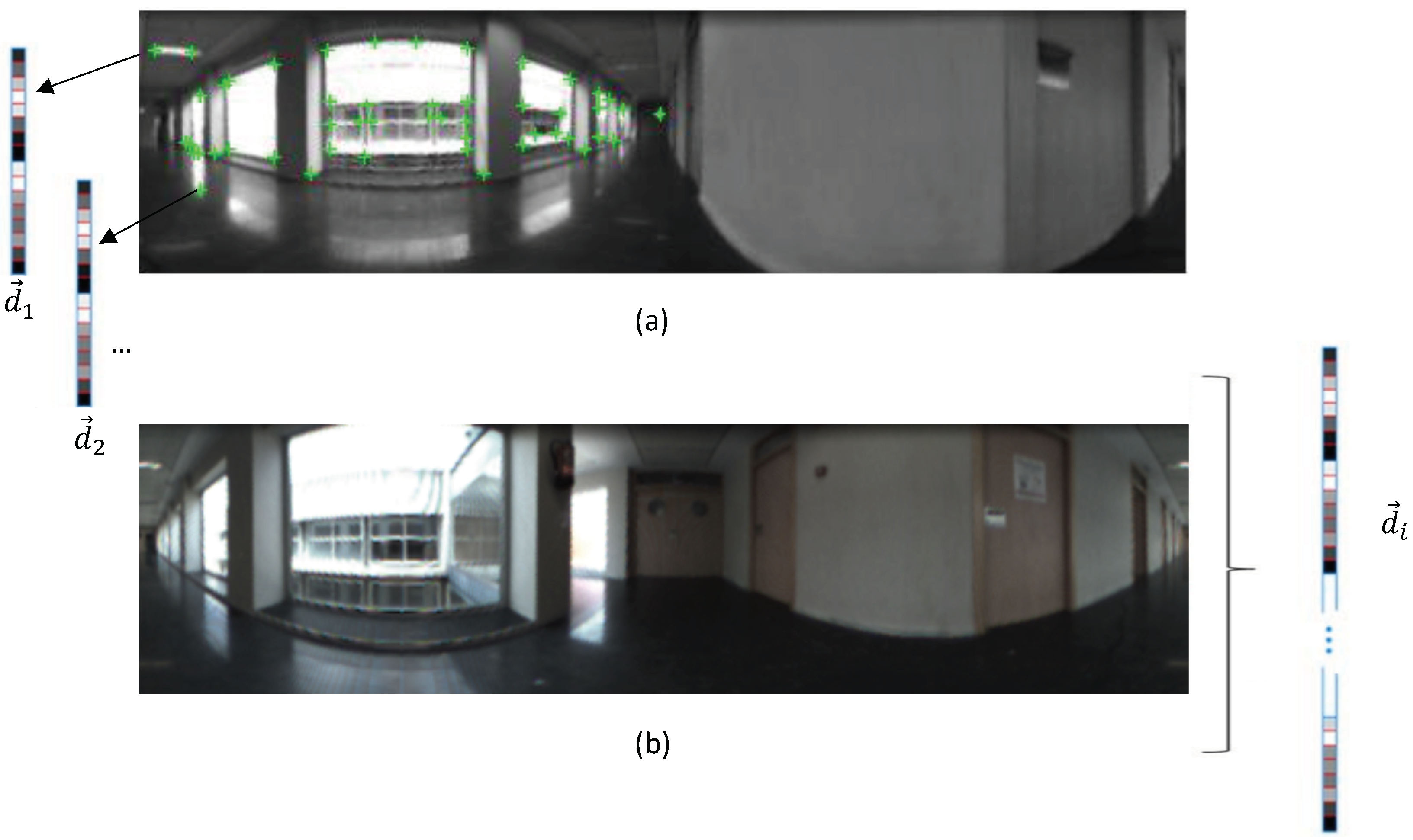
Visual mapping and localization have been solved mainly by using two main approaches to extract the most relevant information from scenes; either by detection, description, and tracking of some relevant landmarks or working with global appearance algorithms, i.e., building a unique descriptor per image. On the one hand, the methods based on local features consist of extracting some outstanding points from each scene and creating a descriptor for each point, using the information around it (Figure 2a). The most popular description methods used for this purpose are SIFT (Scale-Invariant Feature Transform) [14] and SURF (Speeded-Up Robust Features) [15]. More recently, descriptors such as BRIEF (Binary Robust Independent Elementary Features) [16] or ORB (Oriented FAST and Rotated BRIEF) [17] have been proposed, trying to overcome some drawbacks such as the computational time and invariance against rotation. These descriptors have become very popular in visual mapping and localization, and many authors have proposed methods that use them, such as Angeli et al., who employed SIFT [18], or Murillo et al., who used SURF [8]. Nonetheless, these methods present some disadvantages. For instance, to obtain reliable landmarks, the environments must be rich in details. Furthermore, keypoints’ detection is not always robust against changes in the environments (e.g., changes of lighting conditions), and sometimes, the description is not totally invariant to changes in the robot position. Moreover, these approaches might be computationally complex; hence, in those cases, it would not be possible to build models in real time. On the other hand, the methods based on the global appearance of scenes consist of treating each image as a whole. Each image is represented by a unique descriptor, which contains information about its global appearance (Figure 2b). These methods lead to simpler mapping and localization algorithms, due to the fact that each scene is described by only one descriptor. Hence, mapping and localization can be carried out by just storing and comparing the descriptors pairwise. Besides, they could be more robust in dynamic and unstructured environments. However, as drawbacks, these methods present a lack of metric information (they are commonly employed to build topological maps). Visual aliasing also might have a negative impact on the mapping and localization tasks, due to the fact that indoor environments are prone to present repetitive visual structures. Additionally, modelling large environments would require a big amount of images, and this can introduce serious issues when these techniques have to be used in real-time applications. Therefore, global appearance is an intuitive alternative to solve the mapping and localization problem, but its robustness against these issues must be tested. Many authors have addressed mapping and localization using global appearance descriptors (Figure 2b). For instance, Menegatti et al. [19] used the Fourier signature in order to build a visual memory of a relatively small environment from a set of panoramic images. Liu et al. [20] proposed a descriptor based on colour features and geometric information. Through this descriptor, a topological map can be built. Payá et al. [21] proposed a mapping method from global appearance and solved the localization in a probabilistic fashion, using a Monte Carlo approach. Furthermore, they developed a comparative analysis of some description methods. Rituerto et al. [22] proposed the use of the descriptor gist [23,24] to create topological maps from omnidirectional images. More recently, Berenguer et al. [6] proposed the Radon transform [25] as the global appearance descriptor of omnidirectional images and a hierarchical localization method. Through this method, first, a rough localization is obtained; after that, a local topological map of a region is created and used to refine the localization of the robot.

In light of the previous information, in the present paper, the use of hierarchical models is proposed to solve the localization task efficiently. In this sense, compression methods are used as a solution to generate the high-level layers of the hierarchical model. Some authors have used clustering algorithms to carry out the compression task. For instance, Zivkovic et al. [26] used spectral clustering to obtain higher level models, which improved the efficiency of the path-planning. Grudic and Mulligan [27] built topological maps through the use of an unsupervised learning algorithm, which worked with spectral clustering. Valgren et al. [28] tackled an on-line topological mapping through the use of incremental spectral clustering. Štimec et al. [29] used an unsupervised clustering based on the multiple eigenspaces algorithm to carry out topological mapping hierarchically using omnidirectional images. More recently, Shi et al. [30] proposed the use of a differential clustering method to improve the compression of telemetry data.

We propose a method to build hierarchical maps through a combination of clustering methods and global appearance descriptors. We compare the performance of spectral and self-organizing maps’ clustering. In addition, an exhaustive experimental evaluation is carried out to assess the performance of the method in mapping and localization tasks, and we evaluate the influence of the most relevant parameters in the results. This is an interesting problem in the field of mobile robotics because, as pointed out before, global appearance descriptors are a straightforward way of describing visual information, but they contain no metric information, comparing to local-features’ descriptors. Additionally, no deep study to assess the performance of global-appearance descriptors in hierarchical mapping can be found in the literature. The experiments show that the proposal that we present is a feasible alternative to build robust compact maps, despite the phenomenon of visual aliasing, which is present in the sets of images that we have used in the experiments.

The present paper continues and extends the study presented in [31], which is a comparative evaluation in which the performance of some descriptors was assessed to create compact models and estimate the position of the robot. The contributions of the present paper are the following: (a) a new method to compact the visual model is proposed; (b) the trade-off compactness-accuracy-computational cost is addressed, and the performance of the compact models is compared to raw models (with no compaction); (c) a comparison between compression through direct methods and compression through clustering methods to solve the localization task is evaluated; and (d) new indoor environments with different topologies are included in the experimental section.

The remainder of the paper is structured as follows: Section 2 outlines the global appearance descriptors that will be tested throughout the paper. After that, Section 3 shows the clustering approaches used to compress the models. Next, Section 4 presents the method to obtain the localization within the compact models. Section 5 presents the experimental results of clustering and localization and also the discussions about the results. Finally, Section 6 outlines the conclusions and future research lines.

2. Global Appearance Descriptors

As mentioned in the previous section, global appearance descriptors constitute an interesting alternative for mapping and localization. In this work, the robot moves along the floor plane, and it captures images using a hyperbolic mirror, which is mounted over a camera along the vertical axis. This section details three methods to describe the global appearance of a set of panoramic scenes $IM=\{i{m}_1,i{m}_2,\dots ,i{m}_N\}$ where $i{m}_j\in {\mathbb{R}}^{M_x\times M_y}$. After using each description method, a descriptor for each image is calculated; thus, the database is composed of a set of descriptors, $D=\{\overrightarrow{d_1},\overrightarrow{d_2},\dots ,\overrightarrow{d_N}\}$ where each descriptor is $\overrightarrow{d_j}\in {\mathbb{C}}^{l\times 1}$ and corresponds to the image $i{m}_j$.

The remainder of the section presents the global appearance techniques used throughout the paper and the homomorphic filter, which is used as a pre-treatment for the images.

2.1. Fourier Signature Descriptor

The Fourier signature descriptor was firstly used by Menegatti et al. [19] to create an image-based memory for robot navigation. Payá et al. [21] studied the computational cost and the error in localization by using Fourier Signature (FS) and proposed a Monte Carlo approach to solve the localization problem in indoor environments.

This description method is based on the use of the Discrete Fourier Transform (DFT). After calculating the FS of a panoramic image, a new complex matrix is obtained $IM(u,v)$. It can be decomposed into two real matrices, one containing the magnitudes and the other the arguments. The steps to obtain a global appearance descriptor from a panoramic image through the Fourier Signature (FS) are: First, departing from the intensity matrix of the original image, the DFT of each row is calculated. The result is a complex matrix with the same size as the original image ($IM(u,v)\in {\mathbb{C}}^{N_x\times N_y}$). Second, only the $k_1$ first columns of this matrix are retained since the main information is in the low frequency components. Third, the resultant matrix ($IM(u,v)\in {\mathbb{C}}^{N_x\times k_1}$) is decomposed into the magnitudes and arguments matrices. The matrix of magnitudes ($A(u,y)\in {\mathbb{R}}^{N_x\times k_1}$) is invariant against changes of the robot orientation in the movement plane if the image is panoramic. In the last step, the global appearance descriptor is obtained by arranging the $k_1$ columns of the magnitudes matrix in one single column ($\overrightarrow{d}\in {\mathbb{R}}^{N_x·k_1\times 1}$).

2.2. Histogram of Oriented Gradients Descriptor

The Histogram of Oriented Gradients (HOG) is a description method used in computer vision to detect objects. This descriptor is remarkable due to the fact that it is easy to build, leads to successful results in detection tasks, and also requires a low computational cost. It is built from the orientation of the gradient in localized parts of the panoramic image. The development consists of dividing the image into small regions ($k_2$ horizontal cells in this work) and compiling a histogram with b bins for the pixels, which are included inside each cell using their gradient orientation. The combination of this information provides the desired descriptor ($\overrightarrow{d}\in {\mathbb{R}}^{b·k_2\times 1}$). This method has been used by some authors such as Mekonnen et al. [32] to develop a person detection tool, or Dong et al. [33], who proposed an HOG-based multi-stage approach for object detection and pose recognition in the field of service robots. This method was firstly used in mobile robotics by Dalal and Triggs [34] to solve people detection task. Zhu et al. [35] presented an improved version with respect to computational time and efficiency to detect people.

The HOG version proposed in this work is described in detail in [36].

2.3. Gist Descriptor

The gist description was introduced by Oliva et al. [37], and it has been commonly used to recognize scenes. Since then, several versions can be found, which work with different features from the images, such as colour, texture, orientation, etc. [38]. Some researchers have used gist in mobile robotics. For instance, Chang et al. [39] used this global appearance descriptor for localization and navigation. Murillo et al. [40] also used the gist descriptor to solve the localization problem, but in this case, the gist descriptor was a reduced version obtained with Principal Components Analysis (PCA).

The version we use throughout this paper is described in [36] and works with the orientation information obtained through a set of Gabor filters. From the panoramic image, m different resolution levels are obtained. Then, $n_{masks}$ orientation filters are applied over each level. Finally, the pixels of every image are grouped into $k_3$ horizontal blocks, and the information is arranged in a vector ($\overrightarrow{d}\in {\mathbb{R}}^{n_{masks}·m·k_3\times 1}$).

2.4. Homomorphic Filter

In order to solve the localization task, typical situations may happen such as lighting variations and changes in the position of some objects (chairs, tables, open doors, etc.). Hence, descriptors must be robust against these circumstances.

Fernandez et al. [41] showed that some pre-treatments could improve the localization accuracy in indoor environments with different lighting levels. Among the studied techniques, the use of the homomorphic filter [42] can be highlighted. The homomorphic filter permits filtering the luminance and reflectance components from an image separately.

The use of this filter has proven to provide especially good results when it is used in combination with the HOG descriptor [31], whereas in the FS and gist cases, the results were similar to or worse than without this pre-treatment filter. Hence, in the present paper, the following configurations will be used throughout the experiments: FS without filter, HOG with filter, and gist without filter.

3. Clustering Methods to Compact the Visual Information

In this section, the creation of topological models and how to compact them will be addressed. Subsequently, these models will be utilized to solve the localization problem. Only visual information and global appearance descriptors will be used in both tasks. This way, the problem will be addressed through the next two steps.

• Learning: creating a map of the environment and compacting it. A set of omnidirectional images is captured from different positions, and a global appearance descriptor for each image is calculated. After that, a clustering method is used to determine the structure and compact the model.
• Validation: Once the map is built, the robot obtains a new image from an unknown position, calculates the descriptor, and compares it with the set of descriptors obtained in the learning step. Through this comparison, the robot must be able to estimate its position.

Focusing on the learning step, the robot moves around the environment and captures some images from different positions to cover the whole environment. This way, a set of omnidirectional images is collected $I=\{i{m}_1,i{m}_2,\dots ,i{m}_N\}$ where $i{m}_j\in {\mathbb{R}}^{N_x\times N_y}$. After that, a global appearance descriptor is calculated for each image; hence, a set of descriptors is obtained $D=\{\overrightarrow{d_1},\overrightarrow{d_2},\dots ,\overrightarrow{d_N}\}$ where $\overrightarrow{d_j}\in {\mathbb{C}}^{l\times 1}$.

This set of descriptors can be considered as a straightforward model of the environments [43,44], as some previous works do. However, in this mapping strategy, important problems appear when the environment has considerable dimensions. The larger the environment is, the more images have to be captured to model it completely. This leads to the requirement of more computational time and also more memory space in order to process and collect the information related to each captured image and to solve the subsequent localization problem. This way, the model should be compacted in such a way that it retains most of the visual information and permits solving the localization problem efficiently.

In this work, we propose a clustering approach to compact the model, with the objective of creating a two-layer hierarchical structure. The low-level layer is composed of a set of descriptors and, to obtain the high-level layer, this set will be compacted via clustering. Each cluster is characterized by the common attributes of the instances that form that group. This way, the dataset $D=\{\overrightarrow{d_1},\overrightarrow{d_2},\dots ,\overrightarrow{d_N}\}$ is divided into $n_c$ clusters $C=\{C_1,C_2,\dots ,C_{n_c}\}$ under the conditions:

$$\begin{array}{c}\hfill C_i\ne \varnothing ,i=1,\dots ,n_c\\ \hfill \bigcup _{i=0}^m{C}_i=D\\ \hfill C_i\bigcap C_j=\varnothing ,i\ne j,i,j=1,\dots ,n_c.\end{array}$$

(1)

After this, each cluster is reduced to a unique representative descriptor, which is obtained in this work as the average of all the descriptors that compose that cluster. A set of representatives is obtained $R=\{\overrightarrow{r_1},\overrightarrow{r_2},\dots ,\overrightarrow{r_{n_c}}\}$, and therefore, the model is compacted. This set of representatives composes the high-level layer.

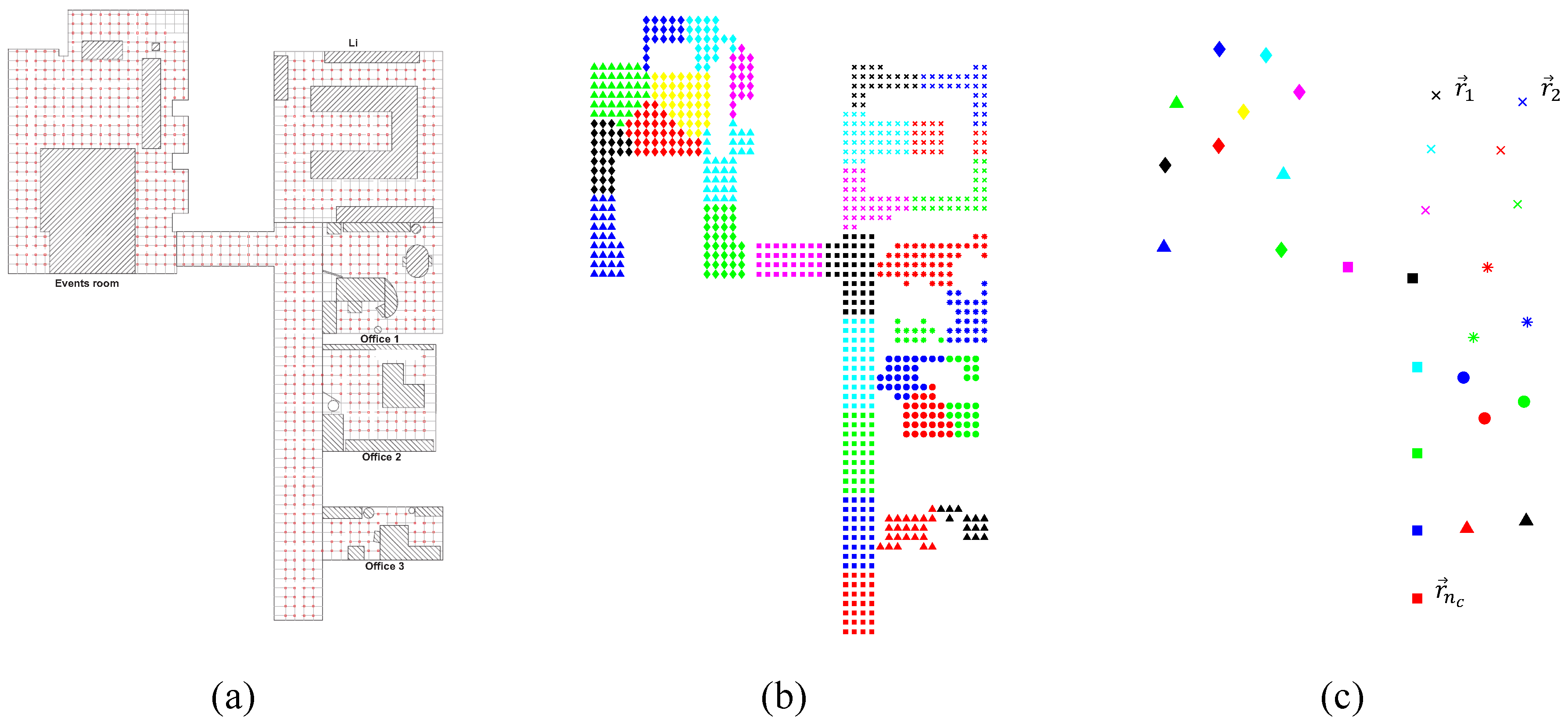
Figure 3 shows how a sample map is compacted. Figure 3a shows the positions where panoramic images were captured to cover the whole environment. The result of the clustering process is presented in Figure 3b, and then, one representative per cluster is obtained (Figure 3c). The representative descriptor is obtained as the average descriptor among those grouped in the same cluster. Additionally, the position of this representative descriptor is calculated as the average position of the capture points of the images included in the same cluster. These positions are calculated just as a ground truth to test the performance of the compact map in a localization process, but they are not used either to build the map, nor to localize the robot. Only visual information is used with these aims. Different clustering methods will be analysed. These methods will only use visual information, and ideally, the objective is to group images captured from near positions despite visual aliasing. To evaluate the correctness of the approach, the geometrical compactness of the clusters and their utility to solve the localization task will be tested in Section 5.

Regarding the clustering process to compact the visual models, two methods are studied: spectral clustering and self-organizing maps.

3.1. Spectral Clustering Algorithm

Spectral clustering algorithms [45] have proven to be suitable to process highly-dimensional data. In this work, a spectral normalized clustering algorithm is used as was introduced by Ng et al. [46]. This algorithm has been already used for mapping along with local features extracted from the scenes [29,47].

In our work, the algorithm departs from the set of global appearance descriptors $D=\{\overrightarrow{d_1},\overrightarrow{d_2},\dots \overrightarrow{d_N}\}$ obtained from the images collected in the environment, and the parameter $n_c$ is the desired number of clusters. Initially, the similitude between descriptors is calculated. This parameter is calculated for each pair of descriptors; hence, a matrix of similitudes S is obtained as $S_{ij}=e^{-\frac{|\overrightarrow{d_i}-\overrightarrow{d_j}{|}^2}{2{\sigma }^2}}$ where $\sigma$ is a parameter that controls the rapidity of the reduction of the similitude when the distance between $\overrightarrow{d_i}$ and $\overrightarrow{d_j}$ increases. The steps to carry out the clustering are the following:

• Calculation of the normalized Laplacian matrix:

  $$L=I-D^{-1/2}S{D}^{1/2}$$

  (2)

  where Dis a diagonal matrix $D_i={\sum }_{j=1}^N{S}_{ij}$.
• Calculation of the $n_c$ main eigenvectors of L, $\{\overrightarrow{u_1},\overrightarrow{u_2},\dots ,\overrightarrow{u_{n_c}}\}$. Arranging these vectors by columns, the matrix $U\in {\mathbb{R}}^{N\times n_c}$ is obtained.
• Normalization of the matrix U to obtain the matrix $T\in {\mathbb{R}}^{N\times n_c}$.
• Extraction of vector ${\overrightarrow{y}}_i\in {\mathbb{R}}^{n_c}$ from the i^th row of the matrix T. $i=1,\dots ,N$.
• Clustering of the ${\overrightarrow{y}}_i$ vectors by using a simple clustering algorithm (such as k-means or hierarchical clustering). Through this, the clusters $A_1,A_2,\dots ,A_{n_c}$ are obtained.
• Obtaining the clusters with the original data as $C_1,C_2,\dots ,C_{n_c}$ where $C_i=\overrightarrow{d_j}$ | $\overrightarrow{y_j}\in A_i$.

If the number of instances N or the dimension l is high, the computation of the $n_c$ eigenvectors (third step) will be computationally expensive. To solve this issue, Luxburg [45] proposed cancelling some components of the similitude matrix. This way, in the matrix S, only the components $S_{ij}$ so that j is among the t nearest neighbours of i are retained. After this, the $n_c$ first eigenvectors of the Laplacian matrix L are calculated by using the Lanczos/Arnoldi factorization [48].

Finally, for each cluster, a representative is obtained as the average visual descriptor of the set of descriptors that compose that cluster.

Spectral clustering may result in being more efficient than traditional methods such as k-means or hierarchical clustering in large environments due to the fact that spectral clustering considers the mutual similitude between the instances.

3.2. Cluster with a Self-Organizing Map Neural Network

As a second alternative, Self-Organizing Maps (SOM) have been chosen to carry out the clustering evaluation in this work. This algorithm was introduced by Kohonen [49], and it is an effective option to carry out a mapping distribution when the data present a high dimensionality [50]. This algorithm has been commonly used for clustering or reducing the dimensionality of data. Therefore, in this work, the input data are the set of global appearance descriptors calculated with one of the methods described in Section 2. The size of the neural network map ($W_{SOM}\times H_{SOM}=n_c$) is chosen. After the training step, the data will be grouped into $n_c$ different clusters.

Self-organizing maps automatically learn to classify input vectors according to their similarity and topology in the input space. They differ from competitive layers in that neighbouring neurons in the SOM learn to recognize neighbouring sections of the input space. Thus, self-organizing maps learn both the distribution (as the competitive layers do) and topology of the input vectors with which they are trained. The neurons can be arranged in a grid, hexagonal, or random topology. The self-organizing map network identifies a wining neuron $i^{\ast }$ using the same procedure as employed by the competitive layer, but instead of updating only the winning neuron, all neurons within a certain neighbourhood $N_{i^{\ast }}\left(d\right)$ of the winning neuron are updated.

4. Using the Compact Topological Maps to Localize the Robot

At this point, the robot is provided with a model of the environment, which, in this case, is a hierarchical map. From it, the robot firstly uses the high-level layer to carry out a rough localization, and secondly, a fine localization is tackled through the use of the low-level layer. The visual localization problem has been solved by many authors through local features by using probabilistic approaches such as particle filters or Monte Carlo localization [51,52]. Nevertheless, the works developed with global appearance descriptors are scarce. Hence, this paper presents a comparison of this kind of descriptor to estimate hierarchically the position of the robot within a hierarchical map in a specific time instant. In order to test the accuracy of the localization method proposed in this work, the coordinates where the images were captured within the environment are known (ground truth). Nevertheless, they are not used to estimate the position of the robot since, as mentioned before, the presented method only considers visual information. This decision permits studying the feasibility of visual sensors as the only source of information to create a compact topological map and, more concisely, of global appearance descriptors. Therefore, not using the position information in the mapping and localization algorithms permits isolating the effect of the main parameters of these descriptors and knowing the performance of this kind of information. The remainder of this section is structured as follows: Section 4.1 outlines the types of distances that have been used to calculate how different the global appearance descriptors are. Section 4.2 explains the localization step within maps that have not been compacted previously, i.e., no clustering has been carried out (the full information about the environment is provided). Finally, Section 4.3 explains the localization task within hierarchical topological maps.

4.1. Distance Measures between Descriptors

In order to know how similar two panoramic images are through their global appearance descriptors, some distance measurements have been used. This way, a comparison can be carried out by calculating the distance between the descriptors of two images captured from different positions of the environment. The lower the distance between those images is, the more similar they are. This kind of distance is used in the localization step. We consider two descriptors $\overrightarrow{a}\in {\mathbb{R}}^{l\times 1}$ and $\overrightarrow{b}\in {\mathbb{R}}^{l\times 1}$, where $a_i$ and $b_i$ are the $i^{\mathrm{th}}$ components of $\overrightarrow{a}$ and $\overrightarrow{b}$ with $i=1,\dots ,l$. The distances used in this work are:

• Euclidean distance: This a particular case of the the weighted metric distance and is defined as:

  $$dis{t}_{euclidean}(\overrightarrow{a},\overrightarrow{b})=\sqrt[]{\sum _{i=1}^l{(a_i-b_i)}^2}$$

  (3)
• Cosine distance: Departing from a similitude metric, which is defined as the scalar product between two vectors, the distance is defined as:

  $$\begin{array}{c}\hfill dis{t}_{cosine}(\overrightarrow{a},\overrightarrow{b})=1-si{m}_{cosine}(\overrightarrow{a},\overrightarrow{b})\\ \hfill si{m}_{cosine}(\overrightarrow{a},\overrightarrow{b})=\frac{{\overrightarrow{a}}^T·\overrightarrow{b}}{|\overrightarrow{a}||\overrightarrow{b}|}\end{array}$$

  (4)
• Correlation distance: Again, departing from a similitude metric, which is defined as a normalized version of the scalar product between two vectors, the distance is defined as:

  $$\begin{array}{c}\hfill dis{t}_{correlation}(\overrightarrow{a},\overrightarrow{b})=1-si{m}_{correlation}(\overrightarrow{a},\overrightarrow{b})\\ \hfill si{m}_{correlation}(\overrightarrow{a},\overrightarrow{b})=\frac{{(\overrightarrow{a}-\overline{a})}^T(\overrightarrow{b}-\overline{b})}{\sqrt[]{{(\overrightarrow{a}-\overline{a})}^T(\overrightarrow{a}-\overline{a})}\sqrt[]{{(\overrightarrow{b}-\overline{b})}^T(\overrightarrow{b}-\overline{b})}}\end{array}$$

  (5)

  where:

  $$\begin{array}{c}\hfill \overline{a}=\frac{1}{l}\sum _{i=1}^l{a}_i;\overline{b}=\frac{1}{l}\sum _{i=1}^l{b}_i\end{array}$$

  (6)

Previous research works [21,36] have evaluated the relation between the distance between the global appearance descriptors and the geometrical distance between capture points. These works show that even if the robot moves a short distance, the descriptor changes. Therefore, global appearance descriptors can be used to detect even small movements.

4.2. Resolution of the Localization Problem in a Model That Has Not Been Compacted

In this case, the map is composed of a straightforward set of descriptors (i.e., this set has not been treated to create a hierarchical map through any clustering process). Once this straightforward map is available, the localization process starts:

• The robot captures a new image at time instant t from an unknown position ($i{m}_t$).
• It calculates the global appearance descriptor of the captured image $\overrightarrow{d_t}$.
• The distances between this new descriptor and the set of descriptors in the map are obtained. The comparison between descriptors is carried out through one of the distance metrics presented in Section 4.1.
• A distance vector $l_t=\{l_{t1},\dots ,l_{tN}\}$ is obtained where $l_{tj}=dist\{\overrightarrow{d_t},\overrightarrow{d_j}\}$ according to any distance measure.
• Considering the position of the robot as the position of the closest neighbour within the map (the problem known as image retrieval [53]), the corresponding position of the robot is the position in the map that minimizes the distance $arg{min}_j{l}_{tj}$. This way, the position $(x,y)$ of the robot in the instant t is estimated.

4.3. Resolution of the Localization Problem in a Compact Model

Image retrieval is an inefficient process due to the fact that the maps are usually composed by a huge number of images and the descriptors have a high dimensionality. Therefore, the computational cost could be a problem. In this case, clustering is used to compact the map. Additionally, indoor environments may present visual aliasing. As explained in Section 3, after clustering, the map $\mathfrak{M}$ will be formed only by a set of clusters $C=\{C_1,\dots ,C_{n_c}\}$, where $n_c$ is the number of clusters. For each cluster, a representative descriptor was calculated as the average of the descriptors in it and the coordinates of those representatives as the average coordinates of the descriptors that compose that cluster. Thus, a set of cluster representatives $\{\overrightarrow{r_1},\dots ,\overrightarrow{r_{n_c}}\}$ and the coordinates of each representative $\{{(x,y)}_{r_1},\dots ,{(x,y)}_{r_{n_c}}\}$ are known (ground truth).

The localization in this hierarchical map is carried out as follows. (1) The robot captures a new image $i{m}_t$ from an unknown position $(x_t,y_t)$, which must be estimated, and (2) the descriptor corresponding to the new captured image is obtained ($\overrightarrow{d_t}$) by using any of the description algorithms explained in Section 2 (FS, HOG, or gist). (3) The distance vector is obtained $l_t=\{l_{t1},\dots ,l_{t{n}_c}\}$ where $l_{tj}=dist\{\overrightarrow{d_t},\overrightarrow{r_j}\}$ is the distance (one of the three types explained in Section 4.1) between the descriptor $\overrightarrow{d_t}$ and each representative $\overrightarrow{r_j}$. Finally, (4) the estimated position of the robot $(x_e,y_e)$ is the position associated with the nearest neighbour $d_t^{nn}|t=arg{min}_j{l}_{tj}$.

The coordinates of the representatives are not used in the localization step. However, to measure the goodness of the estimation, the geometric distance between $(x_t,y_t)$ and the centre of the corresponding cluster (obtained as the average position among the positions of the images that belong to that cluster) is calculated: $error=\sqrt[]{{(x_e-x_t)}^2+{(y_e-y_t)}^2}$. Furthermore, the required computational cost to estimate the localization is calculated.

5. Experiments

5.1. Datasets

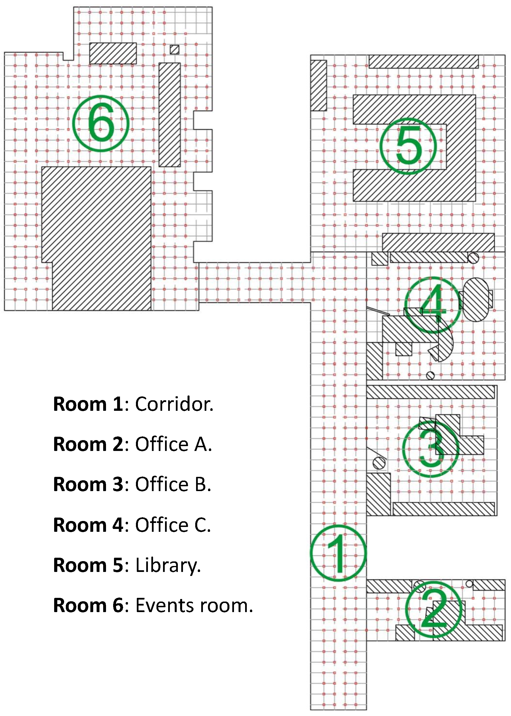
Two different types of datasets were used to develop the experiments; QuorumV, which contains grid-distributed visual data, and the COsy Localization Database (COLD), which contains visual information along a trajectory. On the one hand, Quorum V is a publicly-available dataset [54], which consists of a set of omnidirectional images that have been captured in an indoor environment at Miguel Hernandez University (Spain). The database includes 3 offices, a library, a meeting room, and a corridor. It is composed by two datasets; the first one is a training dataset, and it is composed of 872 images, which were captured on a dense $40\times 40$ cm grid of points. As for the second dataset, the test dataset, it is composed of 77 images, which were captured in different parts of the environment, in half-way positions among the points of the training dataset, and including changes in the environment (e.g., people walking, position of furniture, etc.). 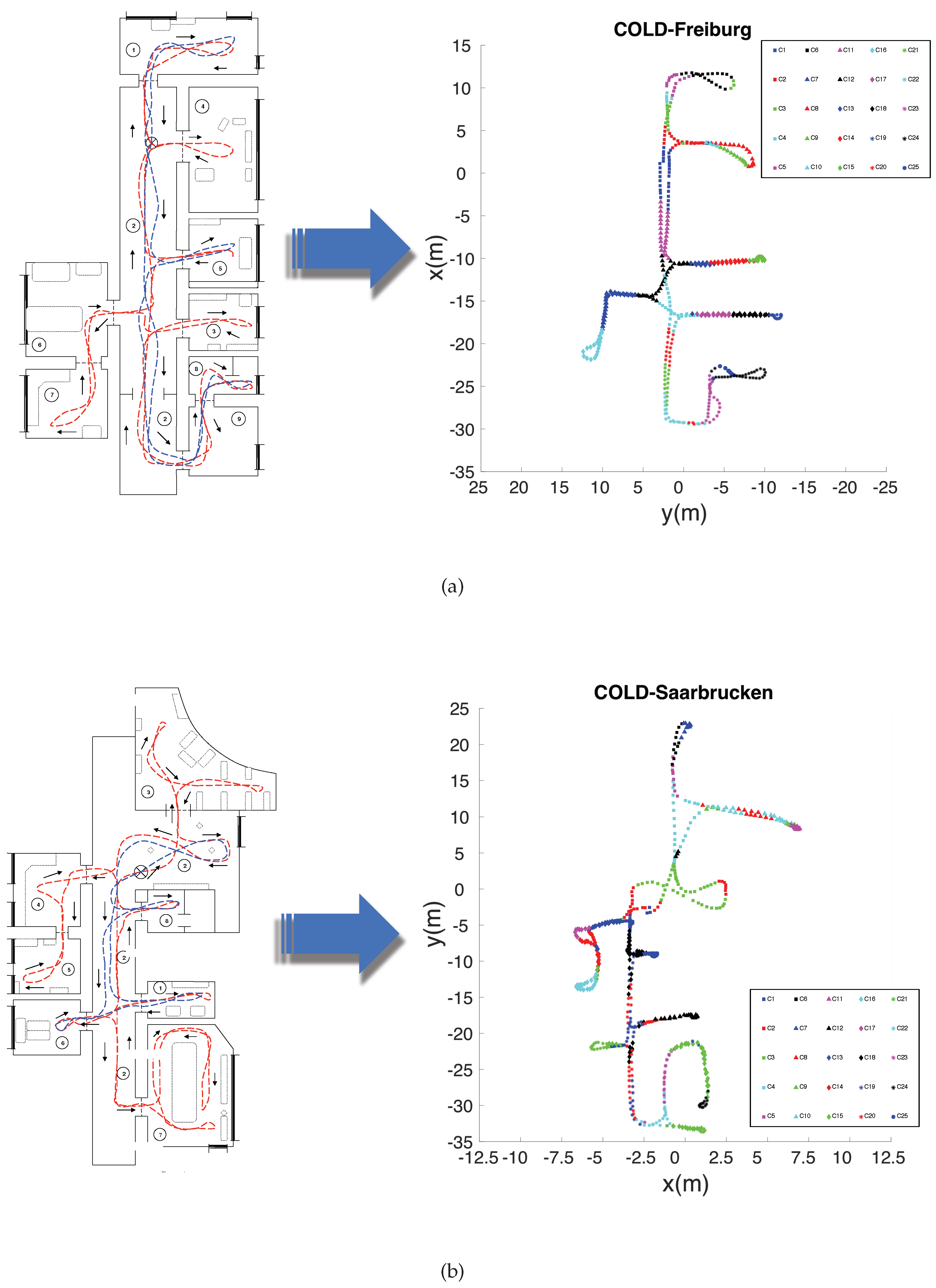Figure 4 shows the bird’s eye view of theQuorum V database and the grid points captured by the robot for the training dataset.

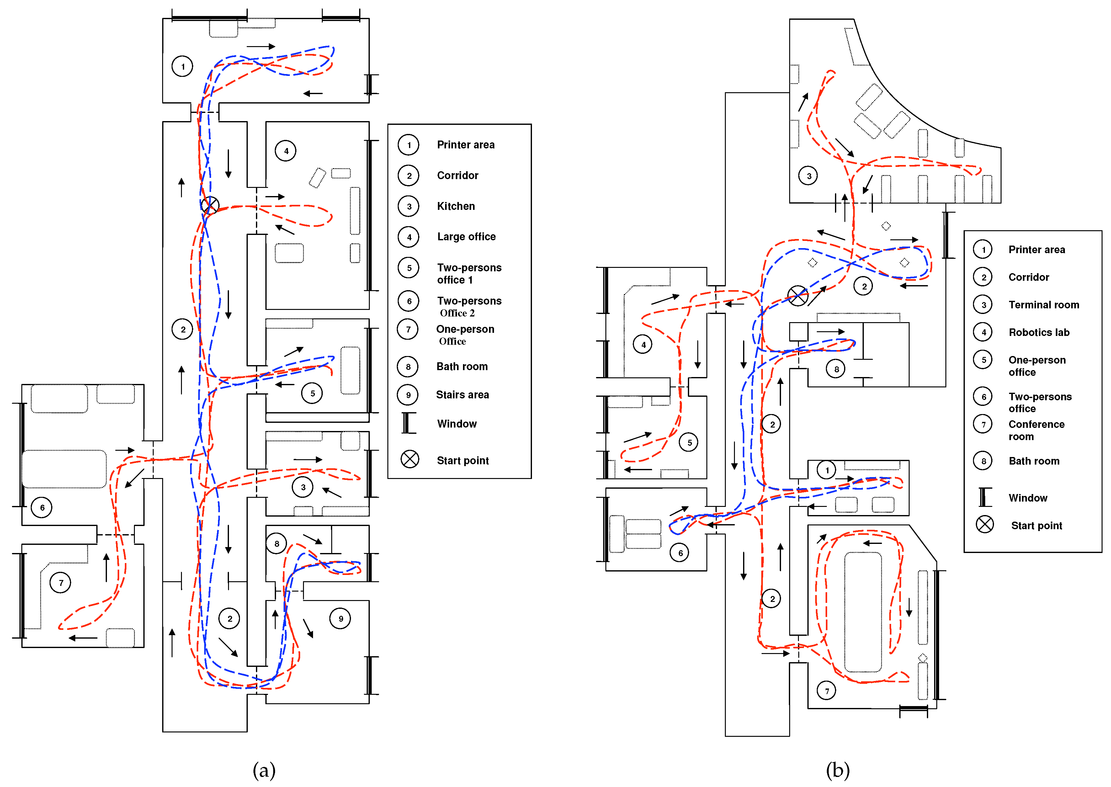
On the other hand, COLD (COsy Localization Database) [55] (also publicly available) contains several sets of images captured in three different indoor environments, which are located in three different cities: Ljubliana (Slovenia), Saarbrücken, and Freiburg (Germany). This database contains omnidirectional images captured while the robot traversed several paths within the environments under real operating conditions (with people that appear and disappear from scenes, changes in the furniture, etc.). In the present work, we use the two longest paths: Saarbrücken and Freiburg. Both datasets include several rooms such as corridors, personal offices, printer areas, kitchens, bathrooms, etc. In order to represent the same distance between images as the distance presented in the Quorum V database, a downsampling is carried out to obtain an acquisition distance between images of 40 cm approximately. Therefore, two training datasets are generated: $Freibur{g}_{training}$ and $Saarbrucke{n}_{training}$, with 519 and 566 images, respectively. Moreover, from the remaining images, test datasets were created. Figure 5 shows the bird’s eye view of the environments and the path that the robot traversed to obtain the images. To summarize,

Table 1. Datasets used to carry out the experiments.

Dataset Name	Number of Images	Number of Rooms
QuorumV_training	872	6
QuorumV_test	77
Freiburg_training	519	9
Freiburg_test	52
Saarbrucken_training	566	8
Saarbrucken_test	57

shows the datasets used for this work and the number of images that each of them contains.

Through evaluating these two types of datasets, an analysis of the localization in maps which are completely different is tackled: the first kind of map (Quorum V) is a grid-based map, and the second dataset (COLD) is a trajectory-based map. The Quorum V database presents a distance between images of 40 cm approximately. This distance is considered reasonable for indoor applications. In this case, the expected maximum error (when all the images are used for mapping) is around 28 cm (a case in which the test image is in the middle of four images of the map, which compose a square of a side of 40 cm). This is a reasonable accuracy to solve localization tasks, and additionally, the requirements of memory to store the images of the map are not excessively high in large environments. Regarding the downsampling that is carried out in COLD, this was done with the purpose of obtaining results that can be directly compared with the ones obtained through the Quorum V database (whose minimum available distance is 40 cm). Previous works [6] have shown that the distance between images has a direct relation with the accuracy of localization when global appearance descriptors are used. Lower distances tend to provide more accurate results. Therefore, if a specific application requires a lower error, a more dense initial dataset of images should be used to obtain the map.

5.2. Creating Compact Maps through Clustering

This section focuses on the evaluation of clustering methods to compact the information contained in a set of global appearance descriptors. To carry out the experiments, two clustering methods were studied for each environment, and three global appearance descriptors were considered. The first method (Method 1) consists of spectral clustering along with k-means as was explained in Section 3.1. Other configurations were tested, such as to use of SOM instead of k-means to solve Step 5 of the spectral clustering, but the results were quite similar; thus, only the spectral clustering along with k-means to cluster the normalized matrix of the $n_c$ eigenvectors is shown. The second method (Method 2) consists of the use of SOM, which was explained in Section 3.2. Therefore, for the two proposed methods, several experiments were carried out to study the influence of the parameters of the three global appearance descriptors.

Table 2. Summary of the parameters that have been varied to carry out the clustering experiments. FS, Fourier Signature.

Parameter	Values
Environment	Quorum V
	Freiburg (COLD)
	Saarbrücken (COLD)
Descriptor	FS
	HOG
	gist
Descriptor parameters	FS: $k_1$ = 4, 8, 16, 32, 64, 128, 256
	HOG: $k_2$ = 2, 4, 16, 32, 64, 128
	gist: $k_3$ = 2, 4, 8, 16, 32, 64
	gist: $n_{masks}$ = 2, 4, 8, 16, 32, 64
Number of clusters	Quorum V: $n_c$ = 15, 25, 40, 60, 80, 100
	Freiburg: $n_c$ = 10, 20, 30, 40, 50, 60, 70
	Saarbrücken: $n_c$ = 10, 20, 30, 40, 50, 60, 70

summarizes the experiments developed.

The values $k_1$, $k_2$, and $k_3$ define the length of each descriptor, but their meaning is not the same (equal values of $k_1$, $k_2$, and $k_3$ would not lead to the same descriptor size). Therefore, as our aim is to study the correct tuning of these values to use each descriptor as efficiently as possible, we do not apply the same values for all the descriptors in the experiments.

Once the compact map has been produced, it may be interesting to provide some measures that permit quantifying the compactness of the map. In this context, the concept of the silhouette is commonly used. Silhouette values point out the degree of similarity between the instances within the same cluster and at the same time the dissimilarity with the instances that belong to other clusters. The silhouette takes values in the range [$-1,1$], and it provides information about how compact the clusters are. Therefore, in order to quantify the goodness of each method, three parameters are considered:

a

The average moment of inertia of the cluster.

b

The average silhouette of the points.

c

The average silhouette of the descriptors.

These values are collected after the clustering process. As for the moment of inertia, it measures the compactness of the clusters (if the clusters group images captured from geometrically-close points) and is calculated as:

$$M=\sum _{i=1}^{n_c}\frac{{\sum }_{j=1}^{n_i}{dist({(x,y)}_{r_i},(x_j,y_j))}^2}{n_i}$$

(7)

where $dist({(x,y)}_{r_i},(x_j,y_j))$ is the Euclidean distance between the coordinates of the representative $r_i$ and the position of the j^th image that belongs to the cluster $C_i$, and $n_i$ is the number of images within this cluster.

As for the silhouettes values, two types of silhouette are used: the average silhouette of points is defined as:

$$S_{points}=\frac{{\sum }_{w=1}^N{s}_w}{N}$$

(8)

N is the number of instances (images), and $s_w$ is the silhouette of each instance; it is calculated as:

$$s_w=\frac{b_w-a_w}{max(a_w,b_w)}$$

(9)

where $a_w$ is the average distance between the capture point of the instance ${\overrightarrow{d}}_w$ and the capture points of the other instances in the same cluster, and $b_w$ is the minimum average distance between the capture point of the instance ${\overrightarrow{d}}_w$ and the capture point of the instances in the other clusters.

Differently, the average silhouette of descriptors is traditionally obtained through:

$$S_{descr}=\frac{{\sum }_{k=1}^N{s}_k}{N}$$

(10)

where N is the total number of instances and $s_k$ is the silhouette of each instance. This value is calculated as:

$$s_k=\frac{b_k-a_k}{max(a_k,b_k)}$$

(11)

where $a_k$ is the average distance between the descriptor ${\overrightarrow{d}}_k$ and the descriptor of the rest of the entities contained in the same cluster, and $b_k$ is the minimum average distance between ${\overrightarrow{d}}_k$ and the instances contained in the other clusters.

The silhouette of descriptors has been traditionally used to measure the compactness of the clusters. However, it does not measure the geometrical compactness. This is why we introduce the silhouette of points, which can provide more proper information since we are interested in knowing whether the clusters have grouped images captured nearby.

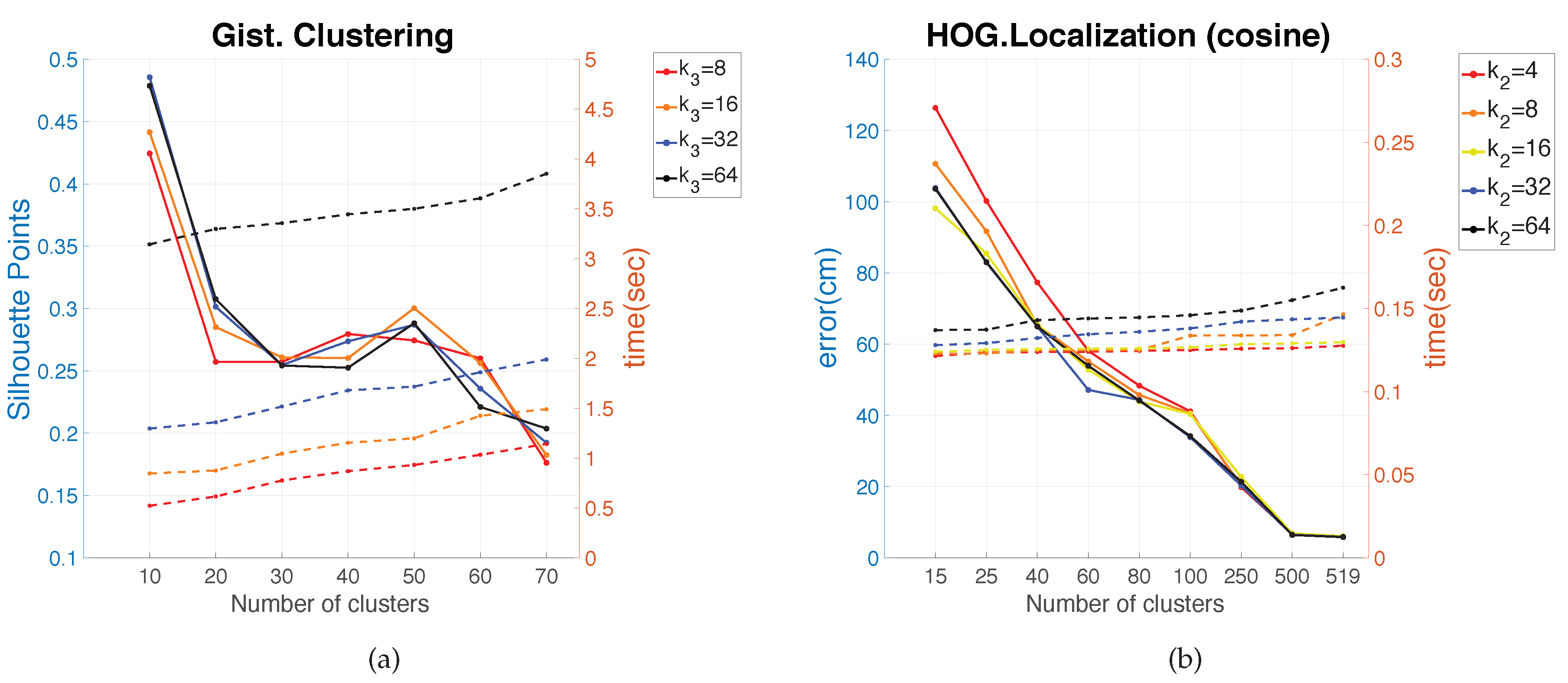
5.2.1. Clustering in the Quorum V Environment

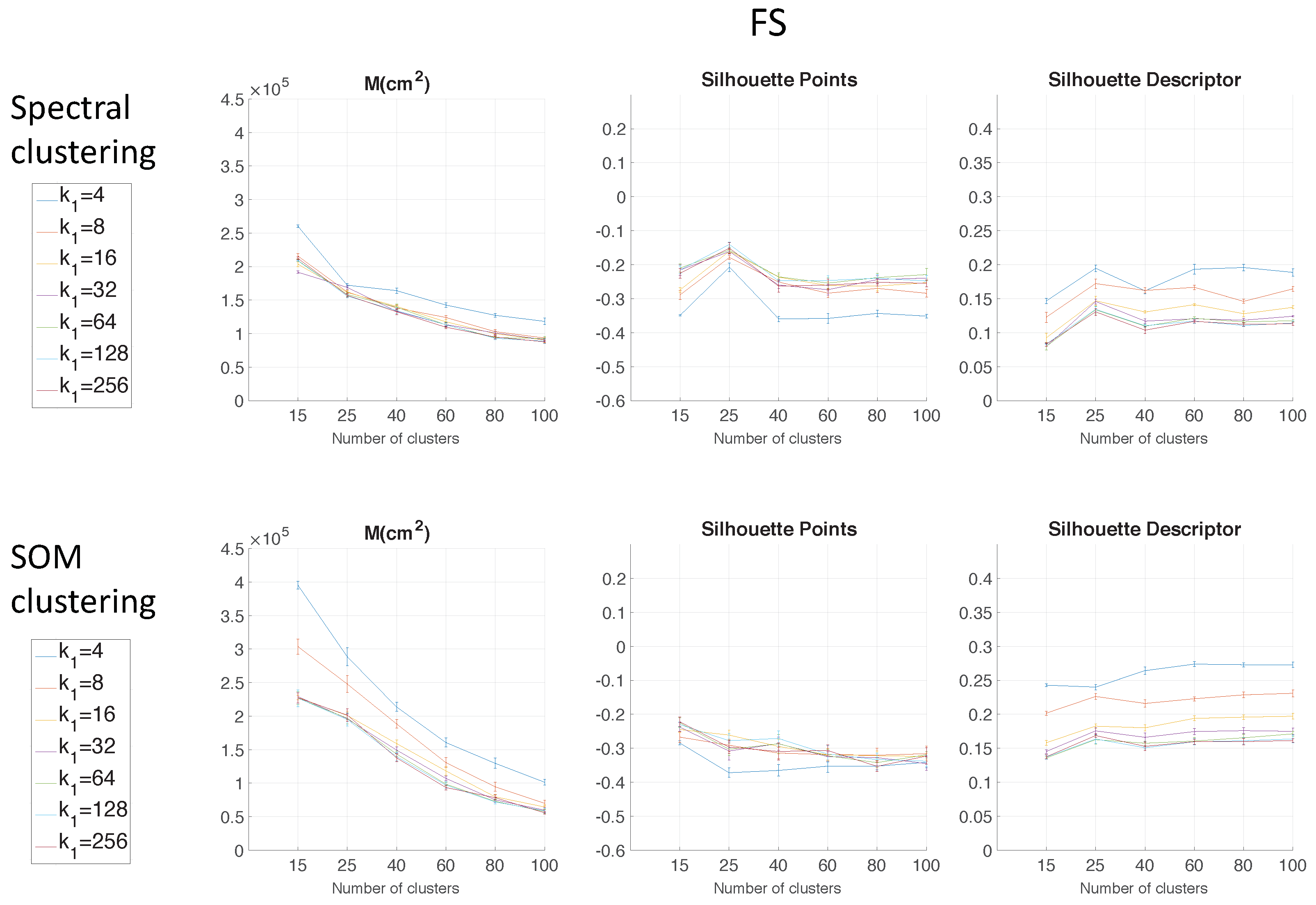
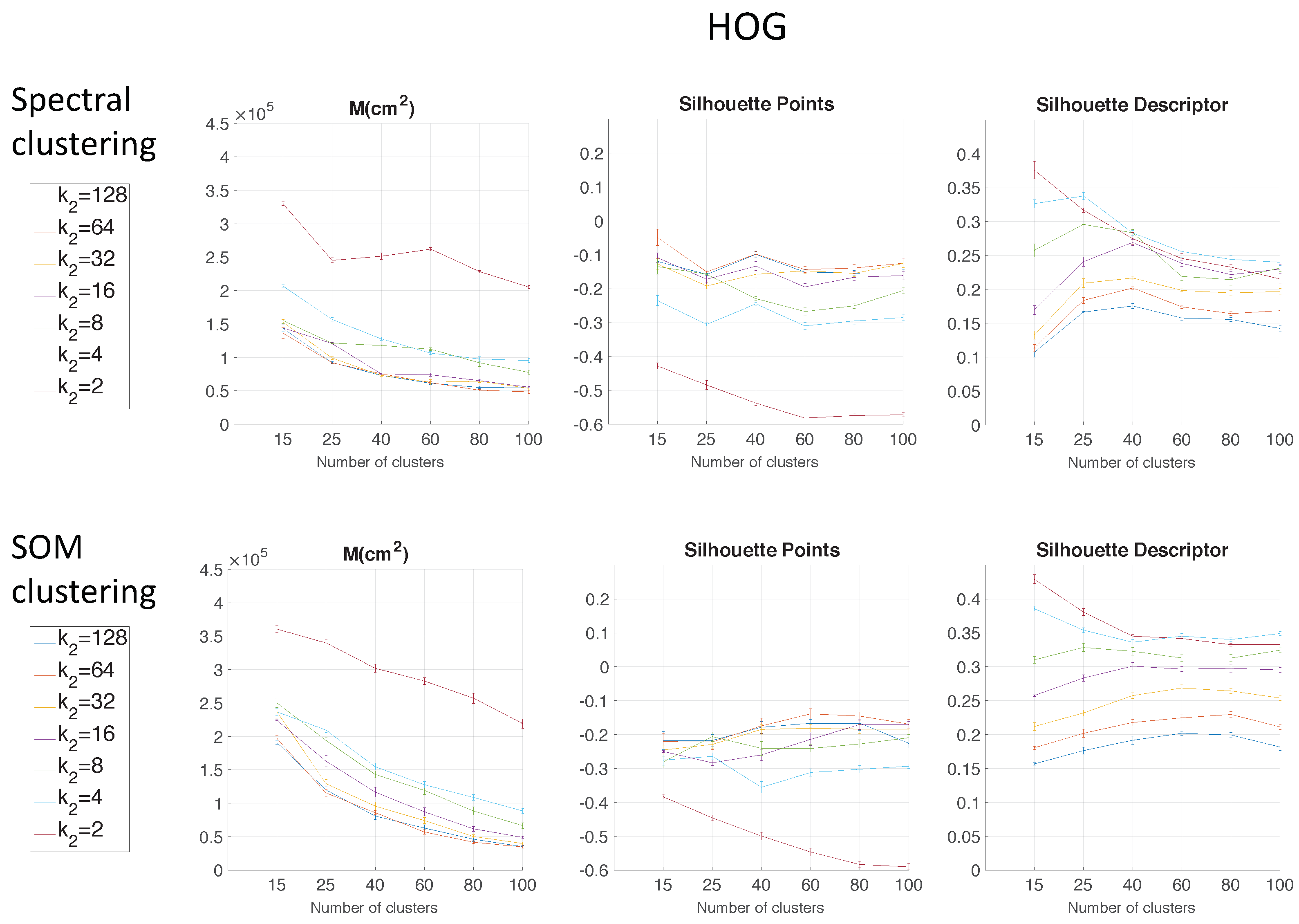
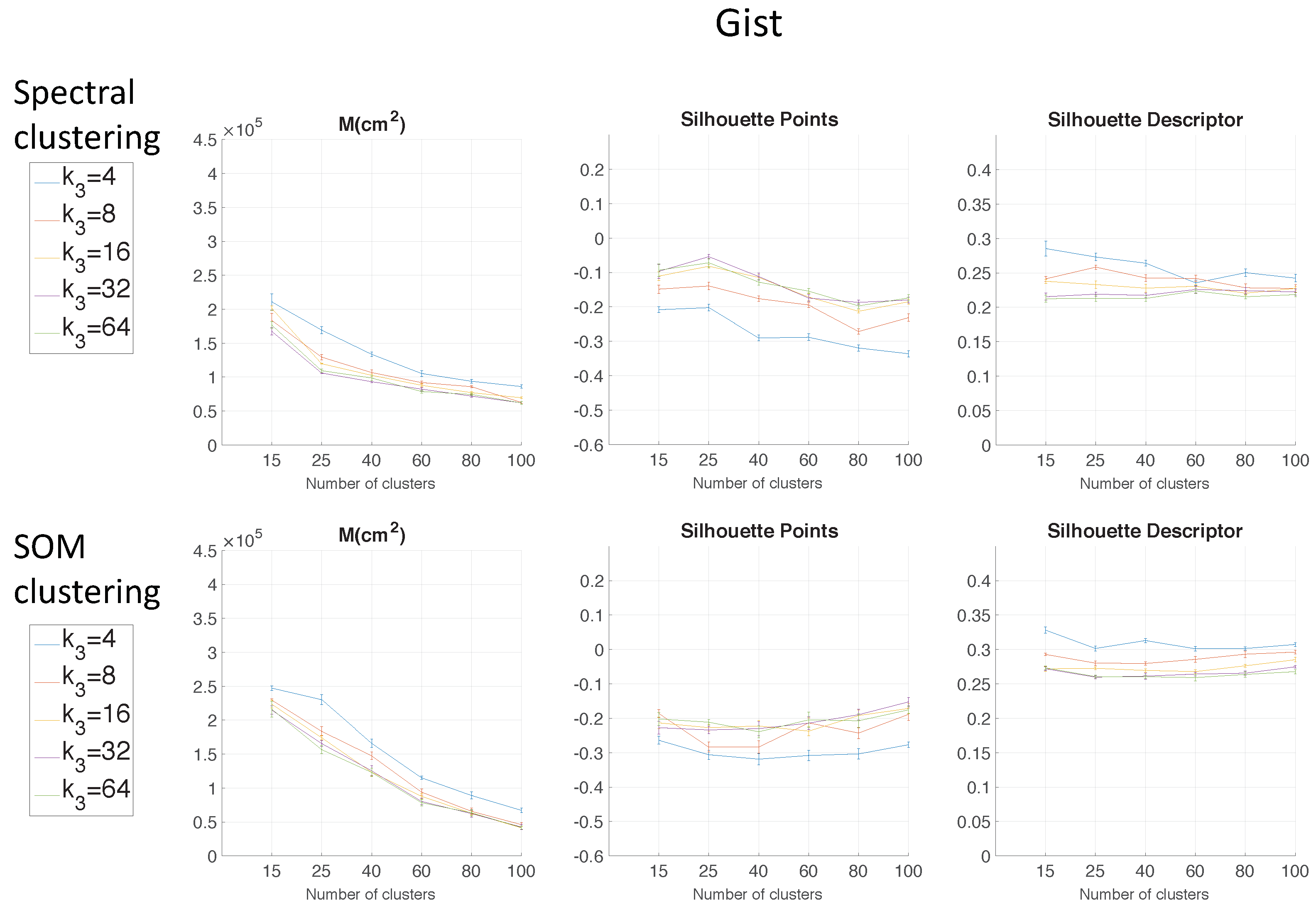
Figure 6 shows the results of the two clustering methods using FS as the descriptor depending on the parameter $k_1$. Figure 7 shows the results using HOG depending on the parameter $k_2$. Figure 8 shows the results using gist depending on the parameter $k_3$ and with $n_{masks}$ = 16. These figures present the graphs that determine the goodness of each configuration to carry out the mapping task through clustering. The three figures show the moment of inertia and average silhouettes vs. the number of clusters. In all cases, the range of the vertical axis is the same, for comparison purposes. 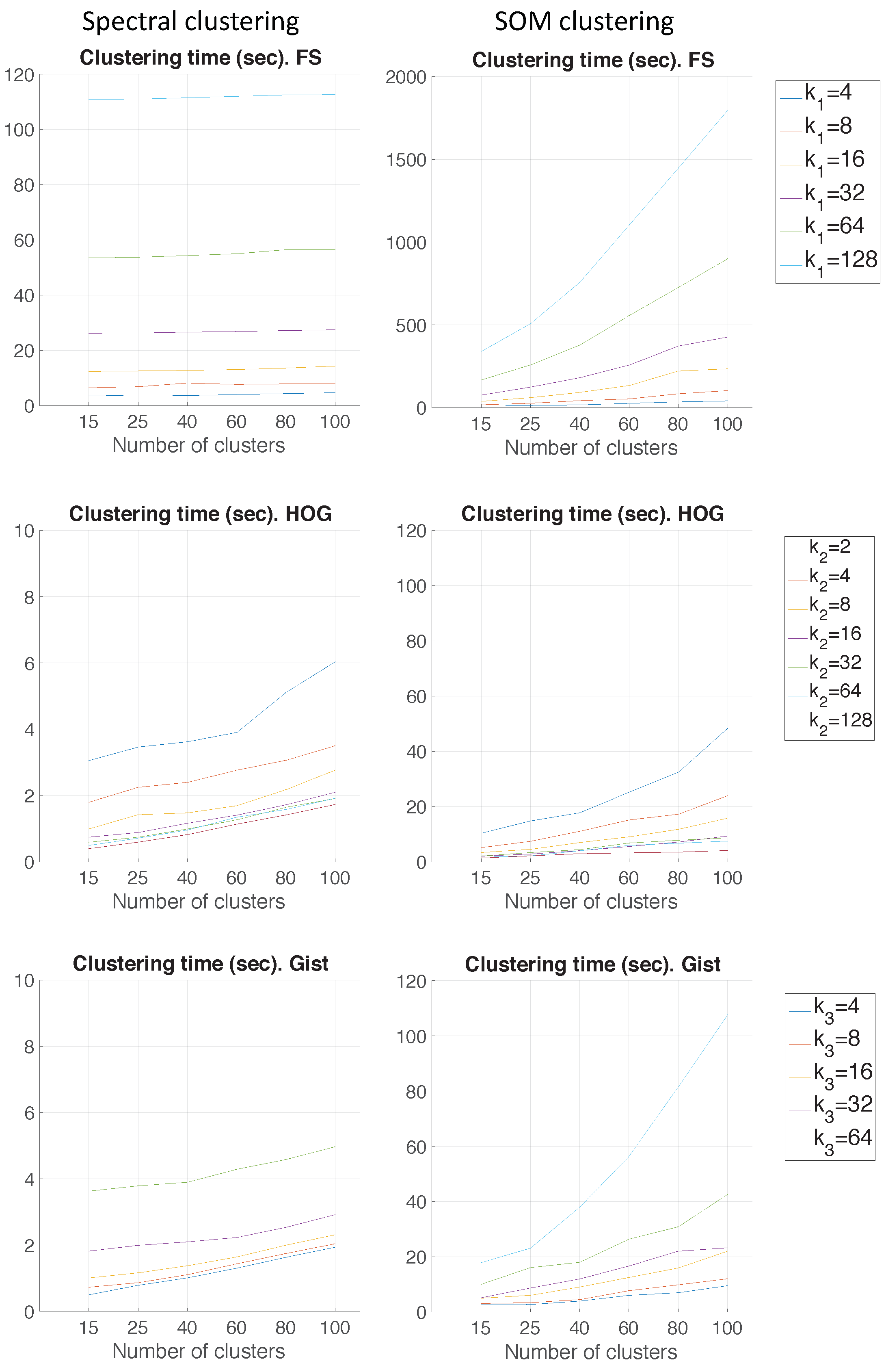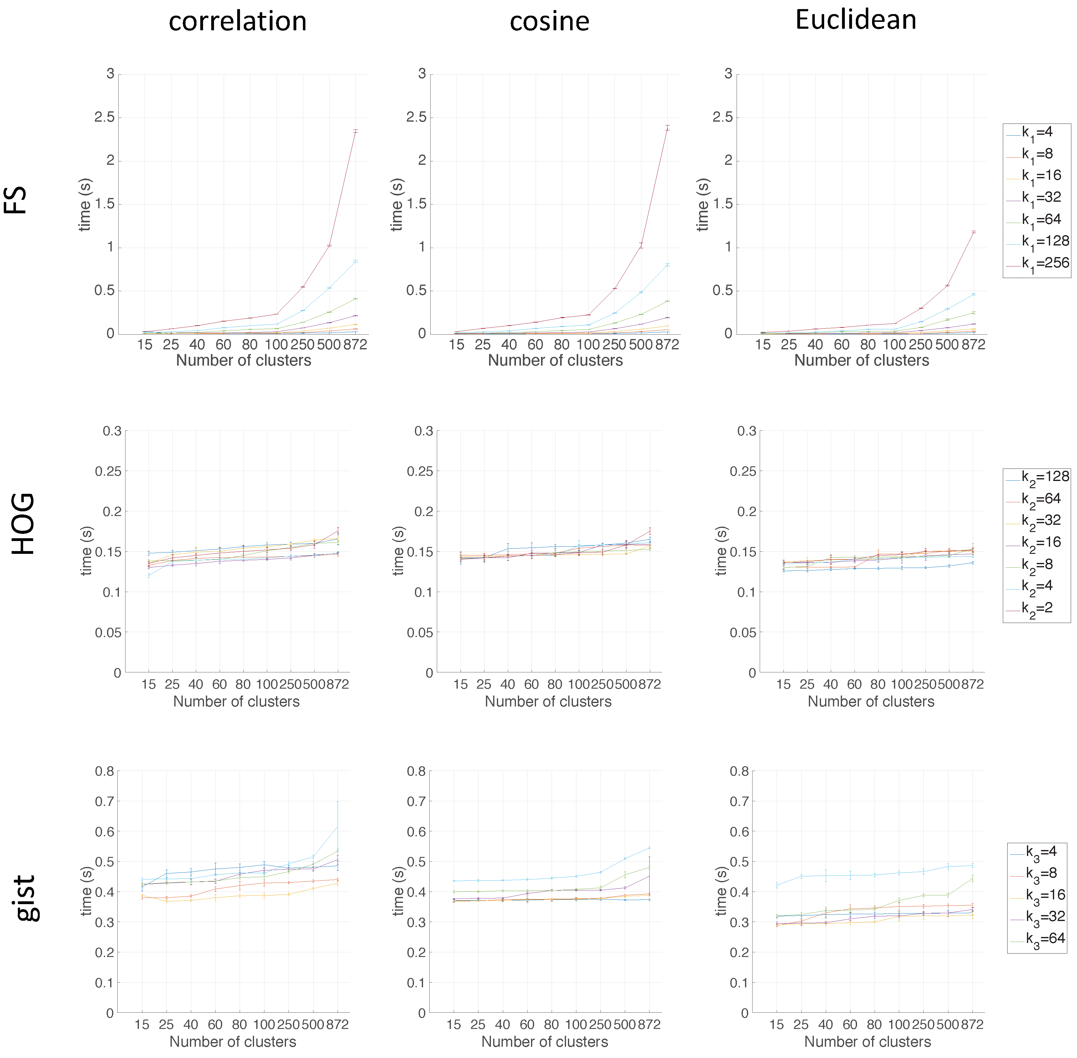Furthermore, Figure 9 shows the computing time necessary to cluster the environment through the two clustering methods.

Regarding the parameters used to measure the compactness of the maps, the lower the moment of inertia and the higher the silhouettes are, the more compact the map is. Generally, Method 1 (spectral clustering) produces the best results. Method 2 (SOM) does not improve these results. As for the use of the global appearance descriptor with the spectral clustering method, FS is not capable of creating reliable clusters. As for HOG, the moment of inertia and silhouettes depend considerably on the value of $k_2$. When $k_2$ is low, the results are poor, but when $k_2>8$, the moment of inertia, as well as the silhouettes improve significantly. At last, regarding the gist descriptor, low values of $k_3$ produce low silhouettes and high moments of inertia, and high values of this parameter imply better results.

As for the computation time required to carry out the clustering through the two methods, the SOM method presents the highest values. The computing time required for the clustering process through the FS descriptor is the highest, whereas the time through HOG or gist is lower, and the fastest one would be determined by the value of either $k_2$ or $k_3$.

As expected, the more components the descriptor has, the more time is required. In Section 5.3, the trade-off descriptor size-localization accuracy will be studied.

Therefore, in the case of HOG, a value of $k_2=32$ or $k_2=64$ could be a good choice to achieve a compromise between compactness and computing time, and in the case of gist, an intermediate value of $k_3$ could be also a good choice for the same purpose. The FS descriptor presents, in general, the worst results: the moment of inertia is higher, and the silhouettes are lower, in general. Hence, the best clustering results are obtained through the use of the spectral clustering method and the use of HOG (for a configuration of $k_2=[32,64]$) or gist (for a configuration of $k_3=[16,32]$ and $n_{masks}=16$) as the global appearance descriptor. Figure 10 shows a bird’s eye view of the clusters obtained with spectral clustering and gistwith $k_3=32$ and $n_{masks}=16$.

5.2.2. Clustering in COLD Environments

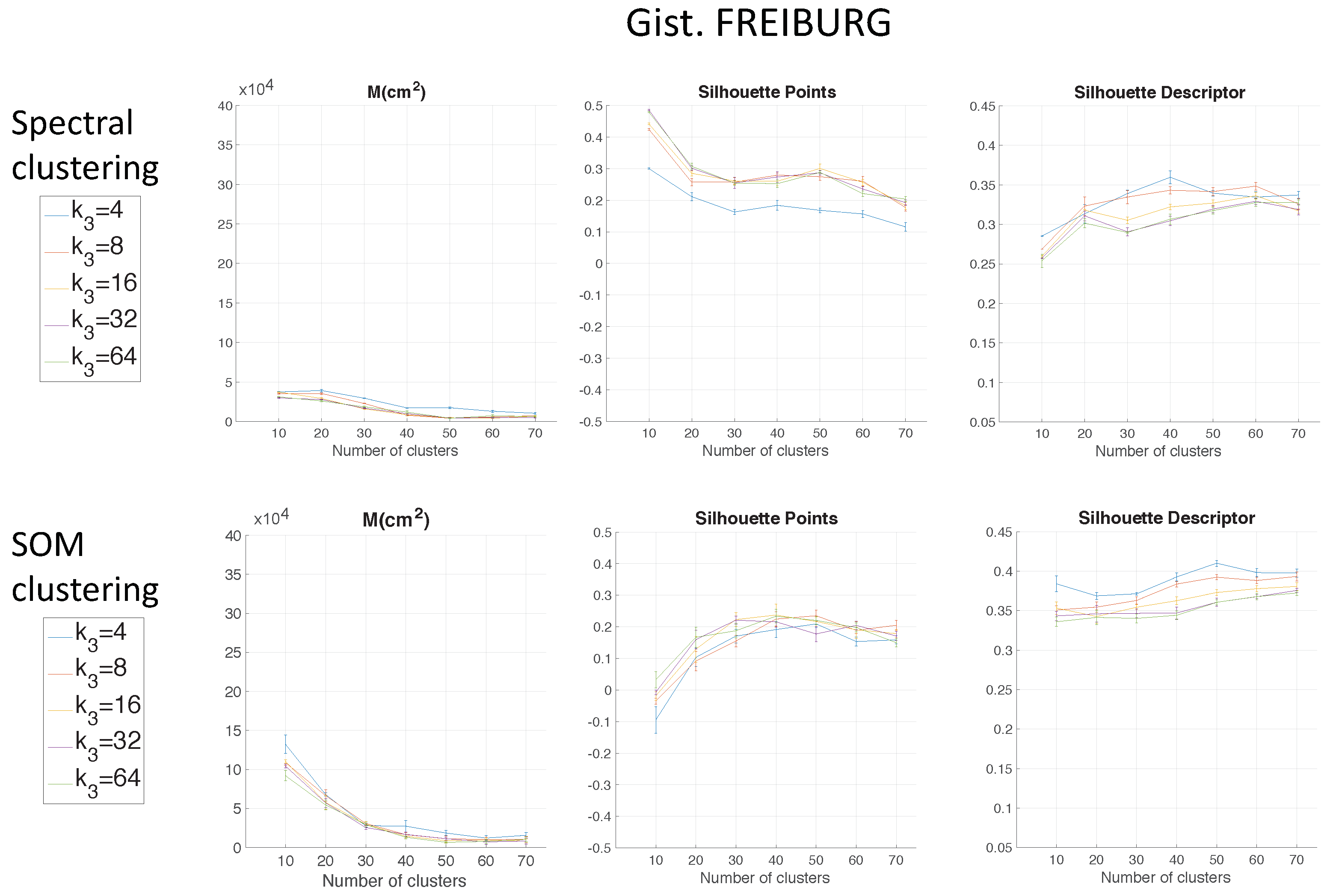
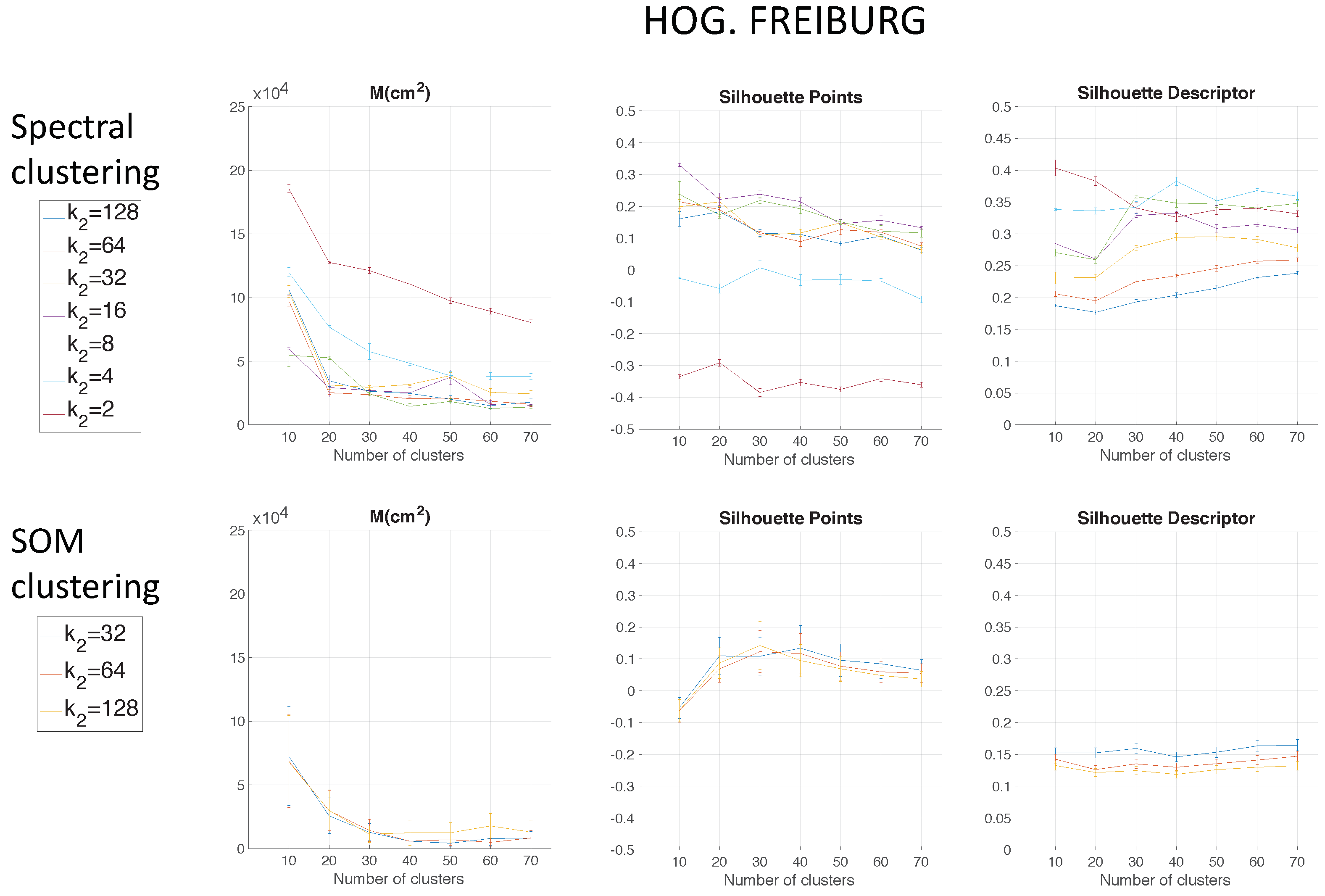
The previous results have shown that the use of FS for clustering is less suitable. Considering this, only HOG and gist descriptors are analysed in the experiments with the COLD environment. Figure 11 shows the results using HOG depending on the parameter $k_2$ in the Freiburg environment. Figure 12 shows the results of the clustering methods using gist depending on the parameter $k_3$ and with $n_{masks}$ = 16 in the Freiburg environment. 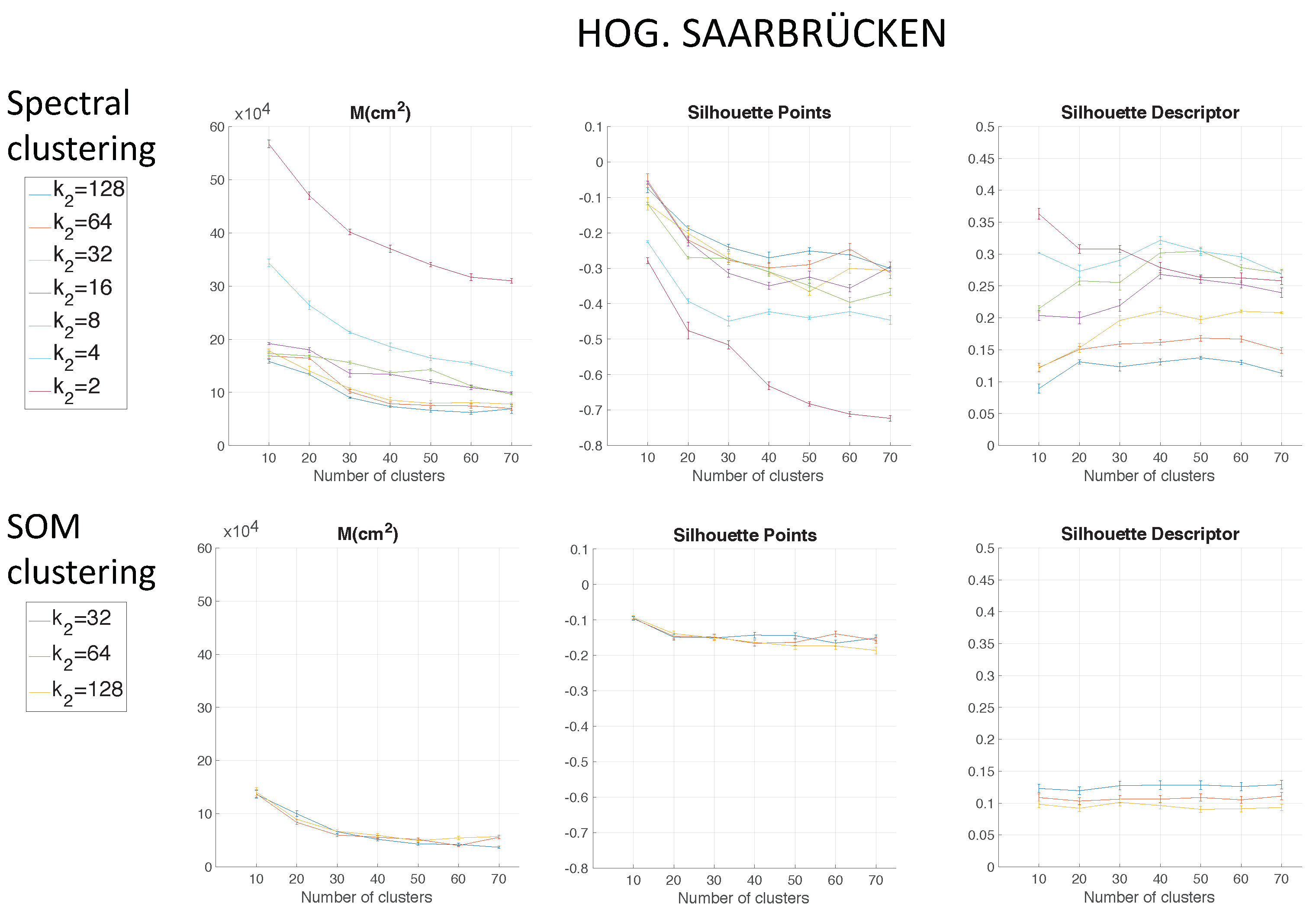In the same way, for the Saarbrücken environment, Figure 13 shows the results using HOG, and Figure 14 shows the results with gist. Regarding the use of HOG with the second method (using SOM), it was not able to solve the clustering task for $k_2=[4,16]$ when $n_c>60$.

Again, spectral clustering is the best method, and in this case, gist presents better clustering outcomes. Hence, through the experiments carried out in the environments of the COLD database, a confirmation of the results obtained in Quorum V is reached (see Figure 15). Therefore, the proposed method is generalizable despite the use of different types of models (linear or grid). As a conclusion, the best option to carry out the compression of visual maps is reached when spectral clustering with gist is applied.

5.3. Localization Using the Compact Maps

This section evaluates the performance of the compact maps to solve the localization problem. The objective is to achieve a compactness that presents a balance between computing time and accuracy of localization. To carry out the evaluation, among the mapping results, the spectral clustering algorithm is selected with the gist descriptor ($k_3=32$ and $n_{masks}=16$). With this configuration, a map per environment is built, using the training images. After that, the test images are used to solve the localization problem. The previous subsection proved that the best option to build the compressed map was through the use of the gist descriptor. Nevertheless, the three proposed global appearance descriptors are proposed again to solve the localization task (because mapping and localization are two independent processes, and the performance of the descriptors could be different in a localization framework). For each test image, its descriptor is calculated (either by FS, HOG, or gist), and then, it is compared with the cluster representatives of the compact map. Afterwards, the most similar cluster is retained. Three distance measures are considered for this comparison: (1) the correlation distance, (2) the cosine distance, and (3) the Euclidean distance. In order to carry out a realistic comparison, despite the real position of the robot being provided by the database, only visual information will be used to estimate the position of the robot. The metric information will be used only as ground truth, for comparison purposes.

5.3.1. Localization in the Quorum V Environment

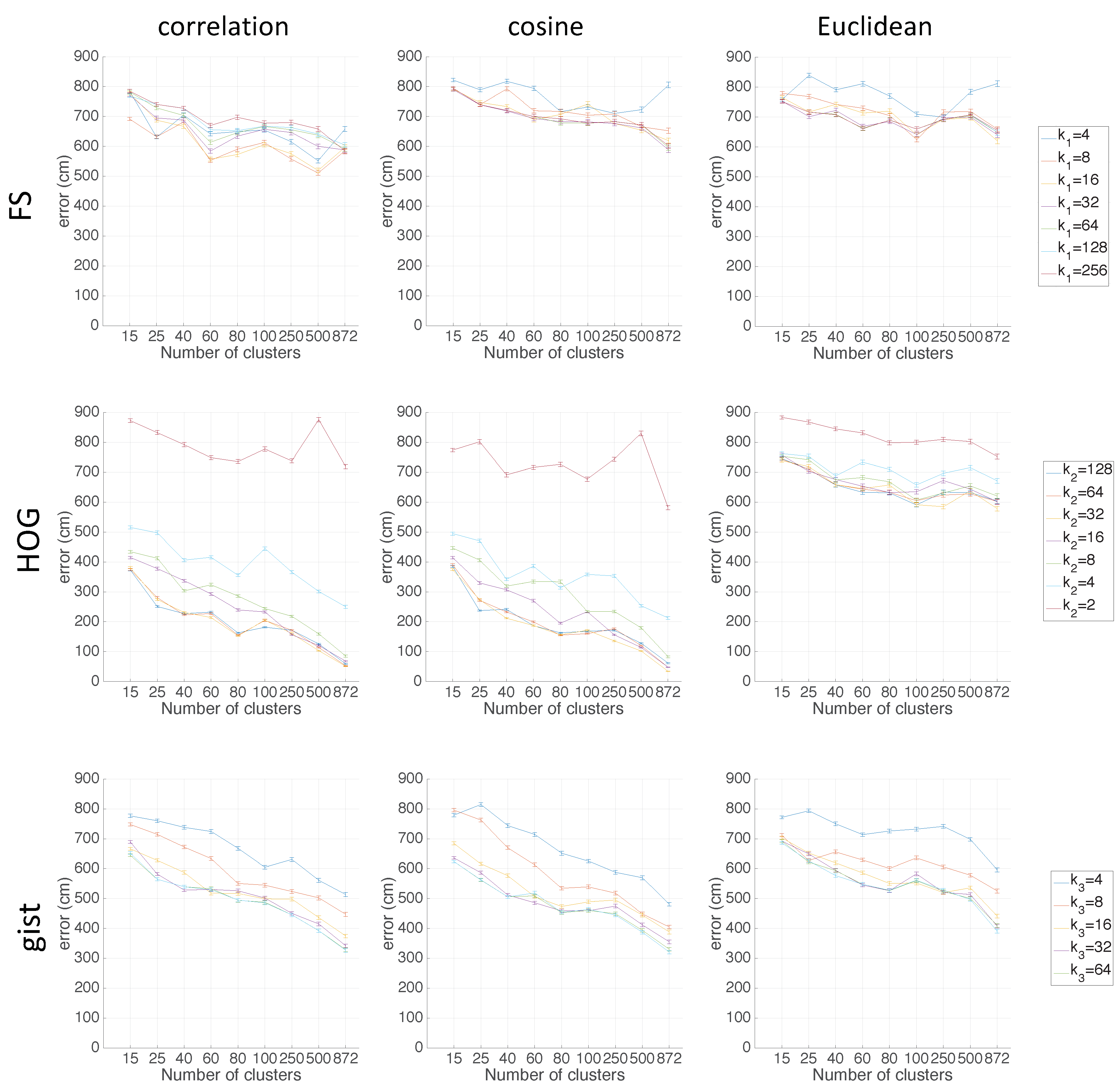
Figure 16 shows the average localization error (cm) obtained when FS (first row), HOG (second row), and gist (third row) are used, respectively, as the descriptor. Figure 17 presents the computational time (s). In the case of HOG, the effect of homomorphic filtering adds a constant time of 0.02 s per test image. Regarding the number of clusters, $n_c=872$ is considered since this value provides the case in which the localization is solved without compacting the map. This value is used as a reference to know the relative utility of the compacted map.

The FS descriptor is not good for localization since the best choice (correlation distance) presents errors between 650 cm and 800 cm depending on the number of clusters and the size of the descriptor. HOG clearly improves the localization task. Except for the case $k_2=2$, the average localization error decreases as the number of clusters increases, and these values go from 500 cm when $n_c$ is low and achieve values under 100 cm (when $n_c$ is high). As for the gist descriptor, it also produces relatively good results, but they are not as good as those obtained through the use of HOG. The localization task achieves the best results when the correlation distance is used.

Regarding the computation time, with the FS descriptor, as the number of clusters increases, the computational time required for the localization task increases substantially. With HOG, the time is much lower than FS, and it keeps constant independently of the number of clusters. This means that the time to calculate the descriptor is higher than the time to compare it with the map. The computation time required for gist is also worse than HOG. The time required by gist is around twice the time with HOG.

In general, as the number of clusters increases, the computation time required for the localization task also increases, and the average localization error decreases. This is an expected behaviour due to the fact that a high number of clusters means that the map is less compact and the information stays in representatives of the clusters whose distance to the test image is lower. Hence, the more clusters, the more comparisons with representatives must be carried out. This leads to a higher computation time and lower average localization error distance. Thus, a balance between these behaviours must be achieved. Therefore, in order to solve the localization in an environment whose properties are similar to the Quorum V environment (grid-distributed data), the optimal values are reached through the use of a HOG descriptor with $k_2=[32,64]$ and correlation distance.

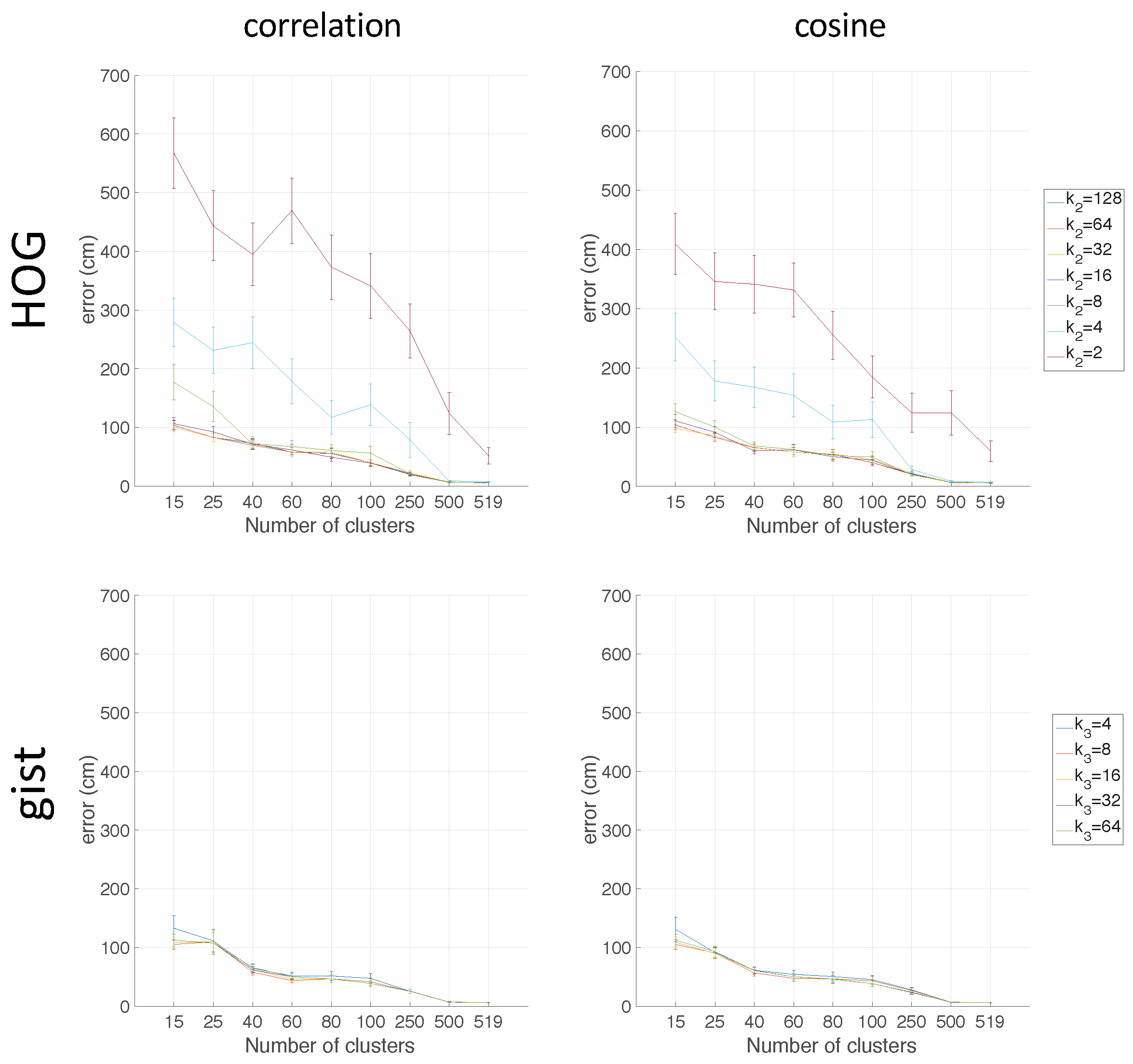
5.3.2. Localization in the Freiburg Environment

As in the previous case (clustering task), with the aim of corroborating the results obtained in Quorum V, an evaluation of the localization task is carried out in the COLD environments. These environments present trajectory maps instead of grid maps. The two COLD environments present a similar configuration and also similar results. This way, only the results obtained in one of them are shown. Freiburg is chosen because this environment presents more rooms and also is more challenging due to the fact that the building presents many glass walls. Moreover, as Figure 16 shows, since the FS descriptor has presented the worst results, this descriptor is discarded in subsequent localization experiments. Furthermore, the Euclidean distance results are omitted in this section because it presented the worst outcomes. Figure 18 shows the average localization error (cm) obtained when HOG (first row) and gist (second row) are used respectively as the descriptor. The case of no compaction is also considered ($n_c=519$).

In this case, some differences are noticed between the results collected in the Quorum V environment and the results in the Freiburg environment. When the number of clusters is low ($n_c=[15,25,40]$), the localization task presents a lower average localization error with gist. If this number is higher than 40, the localization error is very similar for HOG and gist. Comparing the results obtained with the two evaluated types of distances, no remarkable differences are found. Nevertheless, a slight improvement can be noticed when the cosine distance is used. For instance, the average error value when $n_c=40$ in HOG is lower with the cosine than with correlation.

Additionally, the value of $k_2$ in HOG is very important. The average error varies significantly according to it. Therefore, in order to solve the localization in an environment whose properties are similar to Freiburg or Saarbrücken (information along a trajectory), the optimal values are reached through the use of HOG descriptor with $k_2=[16,32]$ and cosine distance.

5.3.3. Localization When Several Maps Are Available

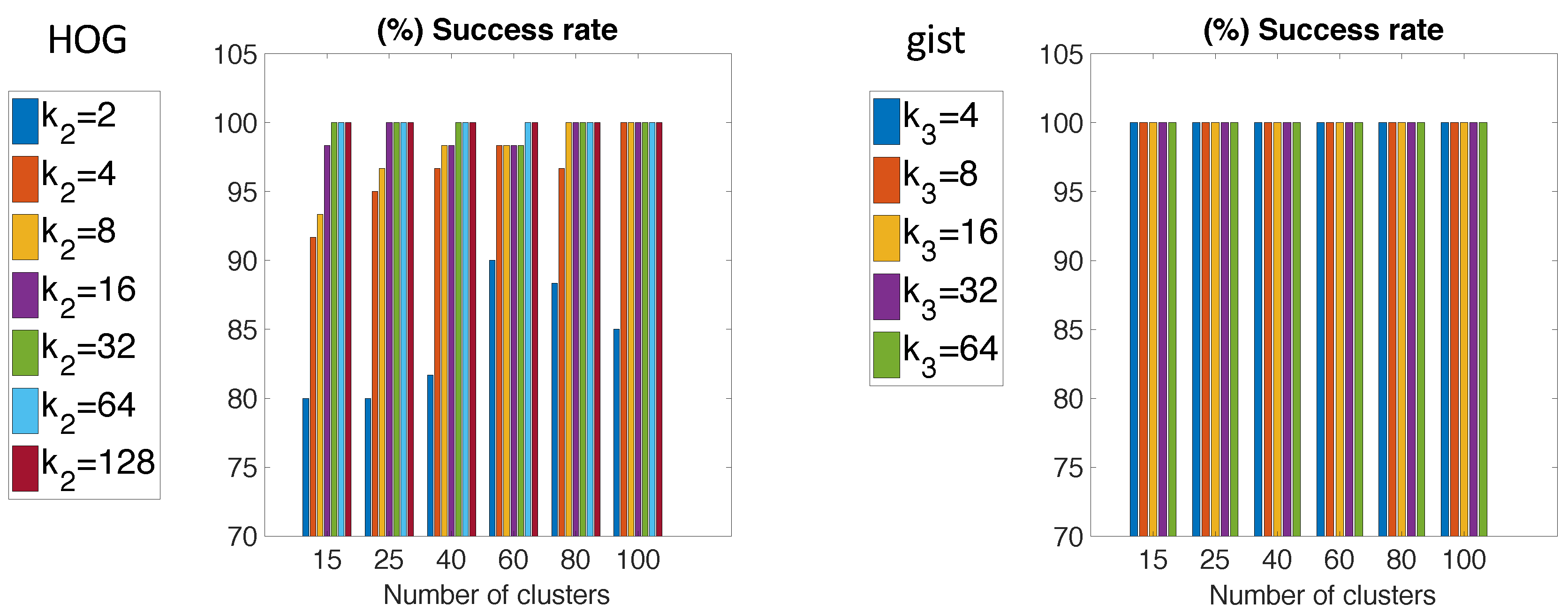
In some applications, several maps of some different environments are initially available. If the robot has no information about the environment it is located in, first, it has to use the visual information to select the correct environment. After that, the localization can be solved in the selected environment, as presented in Section 4. Considering this, in this section, the ability to select the right environment is studied. In order to check the goodness of the descriptors for this purpose, the two COLD maps built in Section 5.2.2 are considered. Additionally, a test dataset is created as a combination of images from the Freiburg and Saarbrüken environments. A total of 60 test images compose the test dataset (34 from Freiburg and 26 from Saarbrücken). In this experiment, only HOG and gist are tested again. Furthermore, since the cosine distance presented the best solutions for COLD, only this kind of distance is applied. Figure 19 shows the percentage of success in selecting the right environment for the two descriptors.

By and large, the correct environment selection is almost always done. Many cases are given in which 100% success is reached, whereas the worst cases do not present a success rate under 75%. If the environment selection is carried out with HOG, results depend substantially on the chosen $k_2$ value. For instance, the worst cases are presented for $k_2=2,4$. However, for $k_2=32-128$, 100% success is reached. Through the use of gist descriptor, 100% success is given independently of the number of clusters or the $k_3$ value.

5.4. A Comparative Study of Localization with Straightforward and with Compact Maps

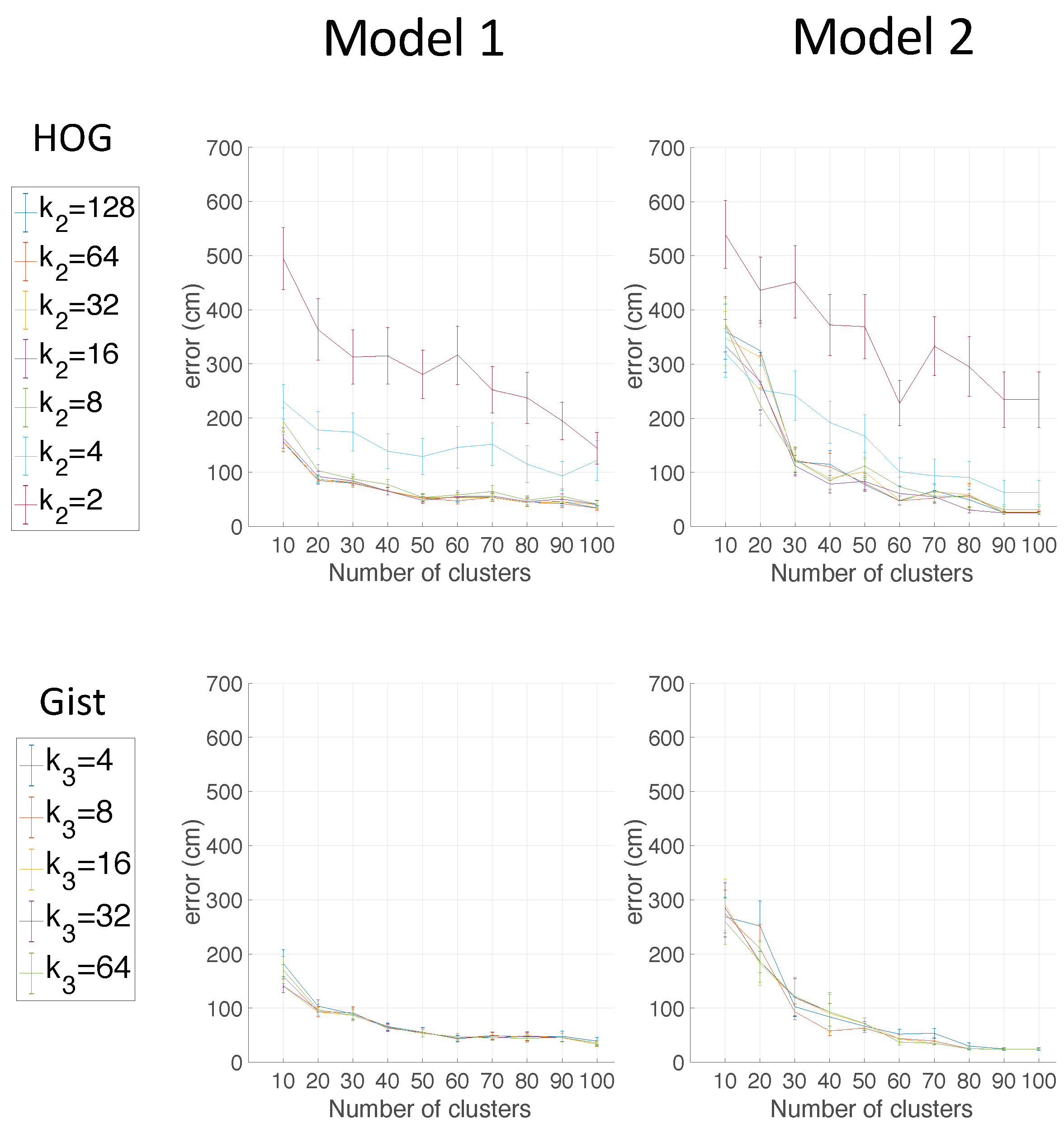
Compact maps obtained after clustering present an effective solution to carry out the localization task in a high-level map, as shown in the previous experiments. This process requires capturing a high number of images from the environment to map, prior to the clustering process. At this point, we could ask the following question: is it necessary to capture this high number of images, or could we create a compact model directly, capturing only a limited number of images from the environment? In this section, this issue is studied. Two kinds of models are considered: (a) a compact model obtained after clustering a high number of images and (b) a straightforward model obtained by just capturing a limited number of views from the environment. Both kinds of models will be used to solve the high-level localization task. The straightforward method we propose to retain representatives is downsampling the databases: the COLD databases are downsampled, and only a certain number of images are retained (one of every x images is retained).

The utility of this straightforward model will be compared with the utility of the optimal compact model obtained in Section 5.2.2 with spectral clustering.

Therefore, two models are used as departing points to carry out the localization task: (Model 1) departing from the representative instances obtained through the spectral clustering algorithm and (Model 2) departing from the instances obtained through sampling the databases. Afterwards, the localization task is studied in the Freiburg environment in the same way as was done in Section 5.3.2.

Figure 20 compares the utility of the two models in localization tasks. The cosine distance is selected to show these results, due to the fact that this distance presented good results in previous localization experiments. The two best global appearance descriptors for localization (HOG and gist) are shown.

As can be seen, the localization error worsens when the straightforward map is used. When the number of clusters is low, the model that has been obtained through spectral clustering presents the best localization results. For example, independent of the descriptor, the average localization error is less than 100 cm when $n_c>20$ for Model 1 and $n_c>40$ for Model 2. The average localization error is lower for Model 2 only when the number of clusters is substantially high, $n_c>80$ (HOG case) and $n_c>70$ (gist case). This outcome means that the proposed alternative to spectral clustering may only be interesting when a low compactness is required. However, if the number of clusters is low (high compactness), spectral clustering provides better results. Therefore, as a conclusion, this experiment has proven that the use of straightforward methods to retain visual representatives is less efficient than using spectral clustering methods. Spectral clustering is able to create compact models that provide accurate localization results.

5.5. Discussion of the Results

This subsection includes a brief discussion related to the results obtained throughout the present work. Regarding the use of methods to compress visual models, spectral clustering has proven to be, in general, more efficient than the SOM clustering. Furthermore, the global appearance descriptor, which presented better behaviour to carry out the clustering task, is gist. About the localization task, HOG presented generally the best outcomes independently of the type of map. The best results are summarized in Figure 21. The best clustering results in Freiburg were obtained with gist ($k_3=[32,64]$ and $n_{masks}=16$) and using spectral clustering. Moreover, the best localization outcome in this environment was obtained through the use of HOG ($k_2=[16,32]$) with the cosine distance.

Furthermore, comparing the localization results obtained after compaction and through using raw models, with no compaction ($n_c=872$, $n_c=519$, and $n_c=566$ respectively for Quorum, Freiburg, and Saarbrücken), compact models have proven to be a successful tool to reduce computing time and keep the localization accuracy (see Section 4).

Regarding the use of the global appearance descriptor to select the right map among several options (Section 5.3.3), gist has proven to be the most efficient choice. Using this descriptor, $100\%$ of success was reached independently of the number of clusters and the value $k_3$.

Finally, straightforward methods to compress the information can be discarded since they are not capable of keeping more information about the environment than the proposed spectral clustering method (Section 5.4). Despite that straightforward methods might be faster and easier, the localization outcomes obtained departing from spectral clustering proved to be, in general terms, more accurate.

6. Conclusions and Future Works

This paper proposes two different methods to compact topological maps. With this aim, three datasets from indoor environments were used. These datasets were composed by either panoramic images or omnidirectional images that were transformed to panoramic. During the experiments, with the objective of compacting the information, the number of instances was reduced to a value in the interval from 10–100. That means a reduction of instances up to between 1.1% and 11.5% of the original number. The proposed methods were (1) spectral clustering and (2) self-organizing maps. Moreover, three global appearance descriptors were used since they presented a good solution for environments whose data dimensionality was high. The work shows that it is possible to reduce the visual information drastically from the original model. Among these combinations of method-descriptor, spectral clustering along with the gist descriptor was proven to be the best choice to compact the model.

Once the original model is compacted, the resultant map can be used to solve the localization task. Hence, an evaluation is carried out with the aim of measuring the goodness of the localization task through the use of compact maps and global appearance descriptors. In this case, three descriptors and two indoor environments are evaluated. Furthermore, a mixture between indoor environments is created with the aim of evaluating whether it is possible, first, to detect the right environment and, second, estimate the position of the instance. From this study, HOG is the description method whose localization results were the best. Additionally, gist presented the most successful results in order to select the correct environment of a test instance from a combined dataset. Finally, the use of clustering methods to tackle the compression step has proven to be more efficient than carrying out a downsampling of the images directly from the database.

The team is now working on how the localization task through compact maps is affected by illumination changes. Additionally, other compacting methods will be studied in order to achieve the Simultaneous Localization And Mapping task (SLAM).