Abstract
Visual–inertial odometry is an effective system for mobile robot navigation. This article presents an egomotion estimation method for a dual-sensor system consisting of a camera and an inertial measurement unit (IMU) based on the cubature information filter and H∞ filter. The intensity of the image was used as the measurement directly. The measurements from the two sensors were fused with a hybrid information filter in a tightly coupled way. The hybrid filter used the third-degree spherical-radial cubature rule in the time-update phase and the fifth-degree spherical simplex-radial cubature rule in the measurement-update phase for numerical stability. The robust H∞ filter was combined into the measurement-update phase of the cubature information filter framework for robustness toward non-Gaussian noises in the intensity measurements. The algorithm was evaluated on a common public dataset and compared to other visual navigation systems in terms of absolute and relative accuracy.
1. Introduction
Visual odometry (VO) is the process of estimating the egomotion of an agent with a single or multiple visual sensors in mobile robot navigation. The aim of VO is to estimate the pose incrementally. Compared with the simultaneous localization and mapping (SLAM) method seeking globally consistent estimation, VO is concerned with the local consistency of the pose estimation [1]. As an inexpensive method independent of external reference systems such as global positioning systems (GPS) and motion capture systems, VO is widely applied in domains including robotics, automotive, and wearable computing [2]. In robotic applications, VO is the basis of studies on visual control [3], obstacle avoidance in robot navigation [4,5], and unmanned aerial vehicle navigation [6].
In practical applications, VO is commonly combined with the inertial measurement units (IMUs) with the aid of Kalman filters. As the visual–inertial integrated navigation system serves as an egomotion estimator and is similar to VO functionally, we used the term of visual–inertial odometry (VIO) in this paper. The IMU generally operates independently of the environmental conditions at a higher rate than cameras. Therefore, the robustness and accuracy of the visual odometry can be enhanced by fusing the IMU measurements.
The VO methods are grouped into indirect methods and direct methods, depending on the usage of the images. The indirect methods preprocess the images of the camera to extract features that are used for motion estimation with a matching process. Direct methods use the raw measurements of the visual sensors without feature extraction and matching processes.
Indirect methods have dominated the research field for a long time, and many effective descriptors of features have been developed as shown in [7]. Guang [8] applied a line-feature extractor in the pre-processing of images and estimated the attitude error with line features. The IMU measurements were fused with the visual measurements loosely with the conventional Kalman filter. Mostafa [9] constructed a multi-sensor fusion system based on the extended Kalman filter (EKF). An indirect VO algorithm with speeded up robust features (SURF) was applied to process the visual measurements. A tightly coupled nonlinear optimization-based indirect VO was applied on the micro aerial vehicle (MAV) in [10,11]. Forster developed a hybrid approach with a direct method for initial alignment and an indirect method for joint optimization. Aladem [12] built a light-weight VO using the adaptive and generic accelerated segment test (AGAST) corner detector and the binary robust independent elementary features (BRIEF) descriptor.
Recently, direct methods have gained more attention due to their independence of extra feature extraction and matching processes. Bloesch [13] used the intensity errors of image patches as measurements and fused the measurements of IMU with the direct VO with EKF. The resulting VIO method was applied in the navigation of a MAV in [14]. Furthermore, Bloesch used the iterated EKF method that operates in a recursive form like the Gauss–Newton optimization to reduce the linearization errors in the regular EKF. A binocular vision system was used to construct a direct VIO in [15]. Engel designed a direct sparse odometry (DSO) using a monocular camera [16]. The even sampling and keyframe management methods used in Engle’s DSO contributed to improving the accuracy and robustness of the photometric-error optimization.
The Jacobian-based EKF method suffers from linearization errors in nonlinear systems. To improve its accuracy, Arasaratnam designed the cubature Kalman filter (CKF) by applying the third-degree spherical-radial cubature rule on the nonlinear Bayes filter [17]. The resulting CKF outperformed the EKF and unscented Kalman filter (UKF) on nonlinear systems. Based on the third-degree CKF, Jia designed a fifth-degree CKF for higher accuracy [18]. Wang developed another CKF method with the regular simplex and moment matching method [19]. The developed fifth-degree spherical simplex-radial cubature Kalman filter (SSRCKF) required fewer cubature points than the fifth-degree CKF in [18] in high-dimensional applications. Zhang developed an arbitrary degree interpolatory cubature Kalman filter (ICKF) with additional free parameters [20]. By adjusting the free parameters, CKF and UKF are special cases of ICKF. An estimator with an online measuring of non-linearity was developed in [21]. The method adaptively switches between cubature rules with different degrees. The CKF was used in [22] for a loosely coupled nonlinear attitude estimator. Tseng [23] embedded the Huber M-estimation method with CKF in [17] to deal with the outliers and non-Gaussian noises in the measurements.
As an equivalent description of the Kalman filter, the information filter has also been extended with the cubature rules for nonlinear systems. Pakki directly applied the technique used in [17] on the information filter and obtained a third-degree spherical-radial cubature rule-based cubature information filter (CIF). Jia applied the fifth-degree spherical-radial cubature rule on the information filter for multi-sensor fusion [24,25]. Yin developed the third-degree spherical simplex-radial cubature information filter. CIFs with different cubature rules have been used in the state estimation for the biased nonlinear system [26], bearing-only tracking with multi sensors [27], and the trajectory estimation for the ballistic missile [28].
The H∞ filter was developed for minimizing the estimation errors in the presence of unsatisfactory noises. Yang developed a solution of the H∞ filter in the form of the regular Kalman filter [29]. Chandra directly embedded Yang’s H∞ filter in the CKF and CIF according to the computational procedures of the filters [30,31] to improve the CKF and CIF in the presence of non-Gaussian noises.
In this paper, motivated by the recently developed cubature information filters for nonlinear systems, a mixed-degree cubature H∞ information filter-based VIO (MCH∞IF-VIO) was designed by fusing the measurements of IMU and intensity errors in a tightly coupled manner. Unlike previous studies that have focused on refining the feature descriptions, we developed the MCH∞IF-VIO system according to the system characteristics and used a simple frame-to-frame alignment model. The proposed VIO method mainly focuses on the nonlinearity and non-Gaussian noises in the VIO system, and is suitable for the camera-IMU system consisting of an IMU and an RGBD camera. The main contributions of this paper are as follows.
- A mixed-degree nonlinear filter framework was proposed for fusing the IMU measurements and the intensity measurements of the camera. The proposed filter applied two cubature rules with different degrees to guarantee numerical stability with high accuracy.
- The H∞ filter was used in the measurement update phase for robustness toward the non-Gaussian noises in intensity errors.
The remainder of this paper is organized as follows. The model of the visual–inertial odometry is presented in Section 2. The VIO system based on a mixed-order cubature H∞ information filter is detailed in Section 3. The test results with a public dataset are presented in Section 4. The conclusions are presented in Section 5.
2. Model of Visual–Inertial Odometry
In this section, we present the model of a keyframe-based VIO system consisting of the motion model, the keyframe management, and the measurement model. The motion model was formulated in form of classical rigid-body kinematics with the modified Rodrigues parameter representing the attitude. The keyframe management was mainly inspired by Engle’s DSO system with some simplifications. The measurement model was formulated in the form of the simple frame-to-frame alignment with the intensity as the measurement.
2.1. Coordinate Systems
Two moving coordinate systems connected with the sensors were used in this paper: (1) The IMU coordinate system (ICS) with its origin at the center of the IMU, where the linear accelerations and angular rates are measured; and (2) The camera coordinate system (CCS) with its origin at the optical center of the camera and the z-axis aligned with the optical axis of the lens.
Another two reference coordinate systems were defined correspondingly: The static IMU coordinate system (SICS) with the same origin and axes as the ICS at the time of constructing the current keyframe; and the static camera coordinate system (SCCS) with the same origin and axes as the CCS at the time of constructing the current keyframe. The SICS and SCCS were static relative to the inertial space in the egomotion estimation.
In this paper, the superscript at the top-left corner of a vector represents the coordinate system the vector is expressed in. Specifically, represents the vector in the ICS, represents the vector in the CCS, represents the vector in the SICS, and represents the vector in the SCCS.
2.2. Motion Model of Camera-IMU System
A 9-dimension system was built to represent the motion of the camera–IMU system. The state vector is defined as follows:
where is the modified Rodrigues parameter (MRP) representing the rotation of the ICS relative to the SICS; is the position of the origin of the ICS in the SICS; and is the velocity of the origin of the ICS relative to the SICS. A discrete motion model was constructed according to the six degrees of the freedom kinematic model of a rigid body as follows:
where is the input vector of the navigation system; and are the measurements of the gyroscope and the accelerator at time , respectively; is a constant vector; is the sampling period; is the gravity acceleration vector in the SICS; is the transformation matrix from the earth-fixed coordinate system to the SICS, of which initial value determined by a simple attitude and heading reference system (AHRS) [32]; and and are the state-transition matrix and input matrix, respectively, formulated as follows:
where is the three-dimensional identity matrix; and is the three-dimensional zero matrix. and are formulated as follows. The right subscript , left subscript ‘SI’ and left prescript ‘I’ in the right side of the equations are neglected to simplify the description
In fact, is the direct cosine matrix representing the rotation of the IMU coordinate system relative to the static IMU coordinate system.
2.3. Keyframe Management
A keyframe consisting of a RGB image and a depth image represents the reference for the egomotion estimation. The very first RGB image and depth image are used to set up the first keyframe. A point set is sampled from the images of the keyframe together with the intensity. Unlike the indirect VO, no extraction or matching process of the distinct features is needed in the direct VO. As a result, the direct VO is generally faster than the indirect VO. However, the accuracy and robustness are hard to ensure without carefully designed features. To ensure the accurate estimation, the point sampling in the direct VO should follow two basic criteria: (1) The sampled points are distributed as evenly as possible in the image; and (2) The absolute intensity gradient at the sampled point is significantly higher than its neighbors. The absolute intensity gradient g at point j with the pixel coordinate of can be evaluated with the intensity differences as follows:
where is the intensity at the corresponding pixel coordinate. For even sampling, the RGB image in the keyframe is divided into patches with the size of . The pixel with the highest absolute intensity gradient among the pixels with valid depth measurements in each patch is chosen as a candidate. If the absolute intensity gradient of a candidate is no less than a predesigned threshold , the 3D coordinate of the candidate pixel is constructed. We used a simple pin-hole camera model for the 3D construction.
where is the depth measurement of corresponding point; and , , , and are the intrinsic parameters of the RGB camera. To simplify the measurement function, the constructed points were transformed into static IMU coordinate system. The transformed 3-dimensional coordinate was added into the point set of the keyframe.
where and represent the transformation between the ICS and the CCS. We assumed that the two sensors were mounted on a rigid body so that the transformation did not change over time. The camera–IMU transformation and the intrinsic parameters were calibrated in advance and the calibration methods are not included in this paper.
The absolute intensity gradient threshold was designed according to the intensity characteristic of each patch and evaluated adaptively online. We treated as the sum of two parts:
where is the average intensity of the image patch and is a positive value to ensure that the absolute intensity gradient of the candidate is sufficiently high. It is easy to understand that the absolute intensity gradient of the candidate should exceed more pixels in a larger patch, which means that is higher with a larger patch and has a positive correlation with the patch size b. We used a simple linear function to represent the positive correlation and formulated the lower-bound constraint of the absolute intensity gradient as follows:
where is a positive constant. Particularly in the case of , i.e., only one pixel exits in each patch, the above lower bound constraint degrades into , which means that all points with valid depth measurements are constructed. Figure 1 shows an example of point sampling on a 640 × 480 image. In the example, the above method was able to sample points not only from the edges of the objects, but also from regions with weak intensity variations such as the computer screen and the floor. The points were distributed more densely with a smaller patch. The numbers of sampled points with different patch sizes in this example are shown in Table 1.
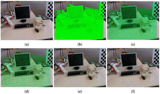
Figure 1.
Example of point sampling on a 640 × 480 image with different patch sizes. The green points represent the sampled points. (a) The original image; (b) The result of point sampling with b = 2; (c) The result of point sampling with b = 4; (d) The result of point sampling with b = 8; (e) The result of point sampling with b = 16; and (f) The result of point sampling with b = 32.

Table 1.
The number of sampled points with different patch sizes.
The above point sampling method adjusts the number of the points by tuning b and guarantees evenly distributed points. The usage of images approximated the dense visual odometry with a small b. The usage of images approximated the sparse visual odometry with a large b. The keyframe may not sufficient to estimate the egomotion as the camera moves, so we used two judging criteria to change the keyframe:
- A new keyframe is needed if there are not enough points in the current view. This is measured via the ratio of points in the current view.
- Observing the same area from different locations far from each other is likely to lead to large differences in occlusion and illumination. In such cases, new keyframes are needed even if enough points are in the current view. This criterion is quantified with the mean square optical flow ignoring rotational motion . is the pixel coordinate of point i in the keyframe, and is the pixel coordinate transformed only by the translational motion.
A new keyframe is constructed with the current RGBD images if any of the two criteria are satisfied. After a new keyframe is constructed, the previous keyframe will be replaced by the new one, and the reference coordinate systems are changed in turn. The estimations of and are transformed with . Then, the estimations of and are set to 0.
The above keyframe and point sampling method mainly refers to Engel’s DSO method, except for several simplifications as follows:
- Only one keyframe is maintained for the sake of complexity.
- The depth measurements are generated with an RGBD camera instead of being estimated in the optimization scheme.
- The gradient constraint in the sampling points is evaluated according to the patch size.
2.4. Measurement Model
A direct VO was used as the measurement model where the intensity was used as the measurement directly without feature extraction and matching processes. The position of each point j was transformed from the SICS into the CCS by the motion state as follows:
The pixel coordinate of point j in the current view was evaluated according to the pin-hole camera model.
The intensity of point j in the RGB image at time k was used as the measurement
where is the measurement noise and assumed to obey a Gaussian distribution with covariance . Combining Equations (11)–(13), one can obtain the following measurement equation.
3. Mixed-Degree Cubature H∞ Information Filter-Based VIO
The above keyframe management method and measurement model of intensity led to a simple frame-to-frame alignment-based egomotion estimator. However, the simple estimator with linearization-based solvers such as the Gaussian–Newton optimization and EKF performed poorly as the models were highly nonlinear and the measurement noises vary dramatically. The linear approximations and Gaussian assumptions used in the solvers were not valid practically. For a robust estimator, the previous studies on VO generally maintained a slide window of multiple keyframes or a local map. In this section, we present a nonlinear filter-based VIO method for the frame-to-frame alignment problem. The designed hybrid cubature H∞ information filter used two cubature rules with different degrees to reduce the linearization error in a numerically stable way and the H∞ filter to estimate the states in the presence of non-Gaussian noises.
3.1. Bayes Filter for Nonlinear Visual–Inertial Navigation System
Consider the following nonlinear system
where and are arbitrary nonlinear functions and and are the process noise and the measurement noise, respectively. Under the Gaussian assumption of noises, the Bayes filter for nonlinear system described by the information vector and information matrix was formulated as an iterated process of a time-update phase and a measurement-update phase.
(1) Time-update phase
(2) Measurement-update phase
The state estimation could be recovered from the information state
According to the measurement model in Equation (14), only a part of the state vector appeared explicitly in the measurement equation. We defined the state vector explicitly shown in the measurement model as follows:
where . The rest state vector is
Correspondingly, the covariance matrix of the state vector is composed of four blocks as follows:
Applying the above partition of the state vector to the evaluation of the predicted measurements (the first equation in Equation (17)), one can obtain.
As shown by Equation (22), the original 9-dimensional integral is simplified to a 6-dimensional integral. The evaluation of the cross-covariance matrix (the second equation in Equation (17)) can also be simplified in a similar way.
where is the joint probability density function of two random vectors and i.e., the probability density function of the Gaussian distribution. Based on the formula of conditional probability, one can obtain
Substituting Equation (24) into Equation (23) yields
With the Gaussian assumption of the state vector, the distribution of conditional on is a multivariate Gaussian with the mean value of and the covariance matrix of . Thus, the inner integral in Equation (25) is solved as
The cross-covariance matrix is evaluated as follows:
In this way, the integrals in 9-dimensional space are simplified into integrals in 6-dimensional space. This is practically useful when applying high-degree cubature rules and will be discussed later.
3.2. Mixed-Degree Cubature Information Filter
In general, the four integrals in Equations (16) and (17) cannot be solved directly. A group of numerical integration-based approximation methods named by cubature rules are used for the filter process and the resulting filters are called cubature filters. Using a cubature rule, a Gaussian weighted integral of a nonlinear function is approximated with a weighted sum as follows:
where represents the cubature points; is the corresponding weight that satisfies ; and is the number of the cubature points. The formulations of the cubature points and weights are different in different cubature rules. The spherical-radial (SR) cubature rules use the spherical-radial coordinates to transform the original integral into a double integral and select the cubature points on the spherical coordinate and the radial coordinate respectively. Based on the SR rules, the spherical simplex-radial (SSR) cubature rules use the n-simplex to evaluate the cubature points on the spherical coordinate.
The degree of a cubature rule is defined based on the degree of used monomials in the Tayler polynomial of the nonlinear function. A p-degree cubature rule integrates all of the monomials in the Tayler polynomial of up to degree p exactly but not exactly for some monomials of degree p + 1. In general, the cubature rule with a higher degree achieves higher accuracy, but suffers from more computation with more cubature points and worse numerical stability with potential negative weights. Practically, third-degree cubature rules and fifth-degree cubature rules are commonly used in the Bayes filter. The numbers of cubature points of the four cubature rules are listed in Table 2.
Table 2.
Number of cubature points of different rules.
A cubature rule with all weights being positive is more desirable than one with both positive and negative weights for the sake of numerical stability. A stability parameter was defined in [33] as the sum of absolute values of the weights:
When is larger than 1, the truncation error will decrease the accuracy of the numerical integration. The curves of with respect to n for different cubature rules are shown in Figure 2. The stability parameters of 3-SR and 3-SSR were maintained at 1, while the stability parameter of 5-SR increased since n > 4, and the stability parameter of 5-SSR increased since n > 7.
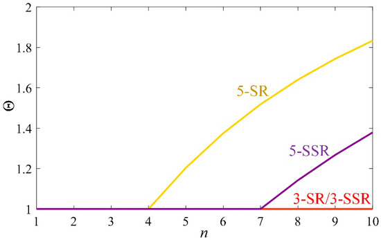
Figure 2.
The curves of with respect to n for different cubature rules.
According to the previous motion and measurement models, the time-update phase involves Gaussian-weighted integrals in 9-dimensional space while the measurement-update phase involves Gaussian-weighted integrals in 6-dimensional space. To obtain high precision and numerical stability with as few cubature points as possible, we applied the 3-SR rule in the time-update phase and the 5-SSR rule in the measurement-update phase. Substituting the chosen cubature rules, we formulated the VIO process based on the mixed-degree cubature information filter as follows.
(1) Time-update phase
Evaluate the cubature points based on the 3-SR rule:
where is the square root of the covariance matrix so that and could be evaluated using the Cholesky decomposition; and is formulated as follows:
Evaluate the predicted state and the covariance matrix:
Evaluate the information matrix and the information vector:
(2) Measurement-update phase
Evaluate the cubature points based on the 5-SSR rule
where is formulated as follows:
where are the vertexes of the -simplex, and
are the projections of the midpoints of the edges constructed by .
The weights for the 5-SSR rule are as follows:
Evaluate the predicted measurement and the cross-covariance matrix :
As the dimension of the measurement vector is generally large, the inversion of the matrix in Equation (17) is very time-consuming. To omit the inversion, we assumed that the m measurements were independent of each other, and the covariance matrix was a diagonal matrix with diagonal elements of . Further assuming that was invariant with time and equal to the other diagonal elements, was treated as a constant . Thus, the inverse of the m × m matrix was replaced by the division of the scalar , and the measurement update of the information vector and matrix was obtained as follows.
Finally, the estimated state vector and covariance matrix were recovered based on Equation (18).
3.3. Robust H∞ Filter
The aim of the H∞ filter is to obtain the state estimation minimizing the following cost function [34].
Based on game theory, the design of the H∞ filter is a game between the filter designer and nature. Nature’s goal is to maximize the estimation error by properly choosing , , and . The cost function is defined in a fractional form to create a fair game by preventing nature using extremely large noises.
The above optimization problem is difficult to solve directly. An alternative strategy is to choose an upper bound and estimate the state satisfying the following constraint.
where is the performance bound to be designed. According to the above equation, a new cost function is defined as follows:
Therefore, the original optimization problem is transformed into the following minimax problem.
Yang [29] solved the minimax problem and proposed an extended H∞ filter (EH∞F) for the nonlinear system, which was similar to EKF in form.
where is the n-dimension identity matrix. The EH∞F is a Jacobian-based filter, and can be extended with cubature rules for higher precision in nonlinear systems as Chandra did in [30]. The time-update phase of the cubature H∞ filter (CH∞F) is the same as the CKF and expressed as the equation. Therefore, we only provided the measurement-update equations as follows:
where the cross-covariance matrix and the measurement matrix are evaluated using a cubature rule. It can be seen from Equations (47) and (48) that the main difference between the EH∞F and the Kalman filter was the formula to update the covariance matrix . In this way, the EH∞F acts to reduce the confidence of the state estimation in case the unexpected noises negatively impact the performance. Applying the information-description of the Kalman filter on the above CH∞F, a cubature H∞ information filter (CH∞IF) can be formulated as follows:
where the covariance matrix of measurement error vector is an m-dimension matrix. As previously stated, m is generally large in direct VO, which means that the inversion of in the above equation is not practical. We used the expressions of the gain matrix in the Kalman filter to simplify the inversion. In this way, the measurement-update phase in CH∞IF was divided into two steps as follows:
(1) Evaluate the measurement matrix with a cubature rule and update the information matrix using the information filter.
(2) Evaluate the gain matrix and execute the measurement update of the H∞ filter.
It is easy to prove that the above two-step measurement-update process is equal to Equation (49). The inversion of the m-dimension matrix is replaced by the inversion of a 9-dimensional matrix .
It is worth noting that the measurement-update phase of the proposed CH∞IF was different to the one with the same abbreviation that Chandra derived in [31]. Compared with Equation (49), Chandra’s method omitted the second term of when using the technique to analyze the estimation error in [35,36]. The error transition function of the measurement-update phase of our method is as follows:
where is the predicted error of the measurement , and formulated as follows:
While the error transition function of the measurement-update phase of Chandra’s method is related to the predicted mean value of the state vector as follows:
This goes against the convergence of the filter. In contrast, the error transition function of our method is in the form of a weighted error function as used in [35,36], which makes a convergent filter.
3.4. Summary of MCH∞IF-Based VIO
Combining the above methods, a mixed-order cubature H∞ information filter (MOCH∞IF) was designed for the nonlinear non-Gaussian VIO system. The time-update phase was the same as Equations (30)–(34). The measurement-update phase was performed in the following steps.
- Evaluate cubature points based on the 5-SSR rule with the time complexity of
- Evaluate the predicted measurements and the cross-covariance matrix with the time complexity of
- Evaluate the measurement matrix with the third equation in Equation (17) and update the information matrix using the information filter with the time complexity of
- Evaluate the gain matrix and execute the measurement update of the H∞ filter with the time complexity of
In conclusion, the time complexity of the measurement-update phase of MOCH∞IF is . In the case of , we have . Generally, the number of measurements is much larger than that i.e., . Thus, the above measurement-update phase is a linear algorithm. In addition, the process of the measurement-update phase is highly parallelizable except for the Cholesky decomposition and the inverse of as it mainly consists of matrix additions and multiplications.
4. Evaluation Results
As analyzed in the previous section, the measurement-update phase with operations of large matrixes is the bottleneck for real-time applications. However, the measurement-update phase of an information-based filter is parallelizable and can be implemented on a parallel processor. We used a laptop with the Geforce 940M GPU (NVIDIA, Santa Clara, CA, USA) and the i7-5600U CPU (Intel, Santa Clara, CA, USA) to test the proposed MOCH∞IF-VIO system. We implemented our method with CUDA (in Supplementary Materials) (Version 8.0, NVIDIA, Santa Clara, CA, USA, 2016) language. The time-update phase was executed on the CPU and the measurement-update phase was executed on the GPU. We used the Technical University of Munich (TUM) RGBD dataset [37] for evaluation. The TUM RGBD dataset contains multiple sequences of videos collected using an RGBD camera under different environmental conditions. The RGB images and depth images are collected at the rate of 30 Hz with a resolution of 640 × 480. The TUM dataset does not contain IMU measurements, we simply used the differential and quadratic differential of the ground truth with the addition of random noises as the simulated IMU measurements.
We compared the proposed MCH∞IF-VIO method with RGBDSLAM v2.0 in [38] and the lightweight visual tracking (LVT) in [12]. The results of RGBDSLAM were calculated with the corresponding ROS package, and the results of the LVT were directly obtained from the original paper. We conducted the evaluation for MCH∞IF-VIO with five different patch sizes: 2, 4, 8, 16, and 32. The numbers were selected as powers of two for the convenience of CUDA implementation. The absolute trajectory (ATE) and relative pose error (RPE) defined in [37] were used as error metrics. The ATE measures the global consistency of the estimated trajectory and is suitable for visual SLAM methods. On the other hand, the RPE measures the local accuracy of the trajectory over a fixed time interval and is suited for visual odometry methods. We used five sequences in the TUM dataset for testing the three methods. The basic parameters of the five sequences are shown in Table 3. The test results are shown in Figure 3, Figure 4, Figure 5, Figure 6 and Figure 7. In these figures, MCH∞IF-VIO(n) represents the MCH∞IF-VIO with a patch size of n.
Table 3.
Parameters of the used sequences.
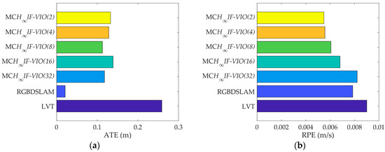
Figure 3.
Test results on the sequence fr1_desk: (a) ATE; (b) RPE.
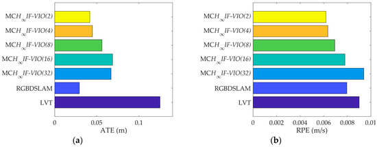
Figure 4.
Test results on the sequence fr1_desk2: (a) ATE; (b) RPE.
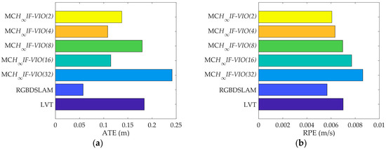
Figure 5.
Test results on the sequence fr1_room: (a) ATE; (b) RPE.
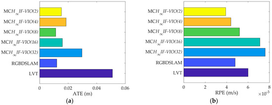
Figure 6.
Test results on the sequence fr1_xyz: (a) ATE; (b) RPE.
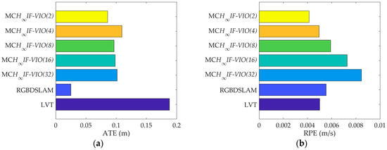
Figure 7.
Test results on the sequence fr3_office: (a) ATE; (b) RPE.
The RPE of MCH∞IF-VIO increased along with the patch size in all of the tests. The change in the ATE of MCH∞IF-VIO was similar to RPE with some exceptions. This is in line with the common knowledge that more measurements lead to better accuracy in visual navigation. The MCH∞IF-VIO in this paper and LVT are dead-reckoning algorithms, while RGBDSLAM is a compete SLAM algorithm with joint optimization and loop-closure. Therefore, RGBDSLAM is more consistent globally than MCH∞IF-VIO and LVT according to the ATE results. In our tests, MCH∞IF-VIO achieved a smaller ATE than LVT with only one exception, where the ATE of MCH∞IF-VIO(32) was larger than LVT in the test on fr1_room. MCH∞IF-VIO(2) had the smallest RPE in all of the tests. The estimation errors caused by the IMU measurement noises increased over time. Moreover, the simple frame-to-frame alignment used in the measurement-update phase was less robust than the optimization with the global and local map used in RGBDSLAM and LVT. Therefore, the performance of MCH∞IF-VIO in the test with long duration such as fr3_office was less distinctive.
5. Conclusions
In this paper, we presented our visual–inertial navigation system called MCH∞IF-VIO, which uses a raw intensity-based measurement model. By analyzing the integrated navigation system, we constructed a numerically stable mixed-degree cubature information filter scheme for the state estimation problem. The H∞ filter was combined for the non-Gaussian noises in the intensity measurements. The proposed VIO system was suitable for the RGBD camera–IMU system. The system was evaluated on the TUM RGBD dataset and compared with the RGBDSLAM and LVT systems.
Given the raw visual measurement model with intensities directly used as measurements in frame-to-frame alignment, the proposed MCH∞IF-VIO system with consideration of the system nonlinearity and non-Gaussian measurement noises was shown to achieve good performance in our tests. Though the method prefers short durations, the implementation with a patch size of two outperformed the RGBDSLAM and LVT in the long-duration test. With the aid of adjustable patch size, the proposed method could be tuned from an accurate-dense algorithm to a fast-sparse algorithm.
This paper aimed to build a robust state-estimation framework according to the fundamental characteristics of the visual–inertial navigation system. The camera measurements were used in a raw and direct way without heuristics in selecting the feature descriptors or tracking a sliding window. Other well-designed intensity-based and feature-based measurement models can be applied in this hybrid filter-based framework.
Supplementary Materials
The CUDA code used in the evaluations is available online at https://1drv.ms/f/s!ApzqIuEnpaPHiDMOyneS8UV2KO6N.
Author Contributions
Investigation, C.S. and X.W.; Methodology, C.S.; Project Administration, X.W.; Resources, N.C.; Software, C.S.; Supervision, N.C.; Writing – Original Draft, C.S.
Funding
This research received no external funding.
Conflicts of Interest
The authors declare no conflict of interest.
References
- Scaramuzza, D.; Fraundorfer, F. Visual odometry part i: The first 30 years and fundamentals. IEEE Robot. Autom. Mag. 2011, 18, 80–92. [Google Scholar] [CrossRef]
- Aqel, M.O.A.; Marhaban, M.H.; Saripan, M.I.; Ismail, N.B. Review of visual odometry: Types, approaches, challenges, and applications. SpringerPlus 2016, 5, 26. [Google Scholar] [CrossRef] [PubMed]
- Papoutsidakis, M.; Kalovrektis, K.; Drosos, C.; Stamoulis, G. Intelligent design and algorithms to control a stereoscopic camera on a robotic workspace. Int. J. Comput. Appl. 2017, 167. [Google Scholar] [CrossRef]
- Basaca-Preciado, L.C.; Sergiyenko, O.Y.; Rodriguez-Quinonez, J.C.; Garcia, X.; Tyrsa, V.V.; Rivas-Lopez, M.; Hernandez-Balbuena, D.; Mercorelli, P.; Podrygalo, M.; Gurko, A.; et al. Optical 3D laser measurement system for navigation of autonomous mobile robot. Opt. Lasers Eng. 2014, 54, 159–169. [Google Scholar] [CrossRef]
- Garcia-Cruz, X.M.; Sergiyenko, O.Y.; Tyrsa, V.; Rivas-Lopez, M.; Hernandez-Balbuena, D.; Rodriguez-Quinonez, J.C.; Basaca-Preciado, L.C.; Mercorelli, P. Optimization of 3D laser scanning speed by use of combined variable step. Opt. Lasers Eng. 2014, 54, 141–151. [Google Scholar] [CrossRef]
- Lindner, L.; Sergiyenko, O.; Rivas-Lopez, M.; Ivanov, M.; Rodriguez-Quinonez, J.C.; Hernandez-Balbuena, D.; Flores-Fuentes, W.; Tyrsa, V.; Muerrieta-Rico, F.N.; Mercorelli, P.; et al. Machine vision system errors for unmanned aerial vehicle navigation. In Proceedings of the 2017 IEEE 26th International Symposium on Industrial Electronics, Edinburgh, UK, 19–21 June 2017; IEEE: New York, NY, USA, 2017; pp. 1615–1620. [Google Scholar]
- Fraundorfer, F.; Scaramuzza, D. Visual odometry part ii: Matching, robustness, optimization, and applications. IEEE Robot. Autom. Mag. 2012, 19, 78–90. [Google Scholar] [CrossRef]
- Guang, X.X.; Gao, Y.B.; Leung, H.; Liu, P.; Li, G.C. An autonomous vehicle navigation system based on inertial and visual sensors. Sensors 2018, 18, 2952. [Google Scholar] [CrossRef]
- Mostafa, M.; Zahran, S.; Moussa, A.; El-Sheimy, N.; Sesay, A. Radar and visual odometry integrated system aided navigation for UAVS in GNSS denied environment. Sensors 2018, 18, 2776. [Google Scholar] [CrossRef]
- Qin, T.; Li, P.L.; Shen, S.J. Vins-mono: A robust and versatile monocular visual-inertial state estimator. IEEE Trans. Robot. 2018, 34, 1004–1020. [Google Scholar] [CrossRef]
- Lin, Y.; Gao, F.; Qin, T.; Gao, W.L.; Liu, T.B.; Wu, W.; Yang, Z.F.; Shen, S.J. Autonomous aerial navigation using monocular visual-inertial fusion. J. Field Robot. 2018, 35, 23–51. [Google Scholar] [CrossRef]
- Aladem, M.; Rawashdeh, S.A. Lightweight visual odometry for autonomous mobile robots. Sensors 2018, 18, 2837. [Google Scholar] [CrossRef] [PubMed]
- Bloesch, M.; Omani, S.; Hutter, M.; Siegwart, R. Robust visual inertial odometry using a direct EKF-based approach. In Proceedings of the 2015 IEEE/RSJ International Conference on Intelligent Robots and Systems, Hamburg, Germany, 28 September–2 October 2015; IEEE: New York, NY, USA, 2015; pp. 298–304. [Google Scholar]
- Sa, I.; Kamel, M.; Burri, M.; Bloesch, M.; Khanna, R.; Popovic, M.; Nieto, J.; Siegwart, R. Build your own visual-inertial drone a cost-effective and open-source autonomous drone. IEEE Robot. Autom. Mag. 2018, 25, 89–103. [Google Scholar] [CrossRef]
- Usenko, V.; Engel, J.; Stuckler, J.; Cremers, D. Direct visual-inertial odometry with stereo cameras. In Proceedings of the 2016 IEEE International Conference on Robotics and Automation, Stockholm, Sweden, 16–21 May 2016; Okamura, A., Menciassi, A., Ude, A., Burschka, D., Lee, D., Arrichiello, F., Liu, H., Moon, H., Neira, J., Sycara, K., et al., Eds.; IEEE: New York, NY, USA, 2016; pp. 1885–1892. [Google Scholar]
- Engel, J.; Koltun, V.; Cremers, D. Direct sparse odometry. IEEE Trans. Pattern Anal. Mach. Intell. 2018, 40, 611–625. [Google Scholar] [CrossRef] [PubMed]
- Arasaratnam, I.; Haykin, S. Cubature kalman filters. IEEE Trans. Autom. Control 2009, 54, 1254–1269. [Google Scholar] [CrossRef]
- Jia, B.; Xin, M.; Cheng, Y. High-degree cubature kalman filter. Automatica 2013, 49, 510–518. [Google Scholar] [CrossRef]
- Wang, S.Y.; Feng, J.C.; Tse, C.K. Spherical simplex-radial cubature kalman filter. IEEE Signal Process. Lett. 2014, 21, 43–46. [Google Scholar] [CrossRef]
- Zhang, Y.G.; Huang, Y.L.; Li, N.; Zhao, L. Interpolatory cubature kalman filters. IET Control Theory Appl. 2015, 9, 1731–1739. [Google Scholar] [CrossRef]
- Zhang, L.; Li, S.; Zhang, E.Z.; Chen, Q.W. Robust measure of non-linearity-based cubature kalman filter. IET Sci. Meas. Technol. 2017, 11, 929–938. [Google Scholar] [CrossRef]
- Guo, X.T.; Sun, C.K.; Wang, P. Multi-rate cubature kalman filter based data fusion method with residual compensation to adapt to sampling rate discrepancy in attitude measurement system. Rev. Sci. Instrum. 2017, 88, 11. [Google Scholar] [CrossRef]
- Tseng, C.H.; Lin, S.F.; Jwo, D.J. Robust huber-based cubature kalman filter for gps navigation processing. J. Navig. 2017, 70, 527–546. [Google Scholar] [CrossRef]
- Bin, J.; Xin, M.; Pham, K.; Blasch, E.; Chen, G.S. Multiple sensor estimation using a high-degree cubature information filter. In Sensors and Systems for Space Applications VI; Pham, K.D., Cox, J.L., Howard, R.T., Chen, G., Eds.; Spie-Int Soc Optical Engineering: Bellingham, WA, USA, 2013; Volume 8739. [Google Scholar]
- Jia, B.; Xin, M. Multiple sensor estimation using a new fifth-degree cubature information filter. Trans. Inst. Meas. Control 2015, 37, 15–24. [Google Scholar] [CrossRef]
- Zhang, L.; Rao, W.B.; Xu, D.X.; Wang, H.L. Two-stage high-degree cubature information filter. J. Intell. Fuzzy Syst. 2017, 33, 2823–2835. [Google Scholar] [CrossRef]
- Jiang, H.; Cai, Y. Adaptive fifth-degree cubature information filter for multi-sensor bearings-only tracking. Sensors 2018, 18, 3241. [Google Scholar] [CrossRef] [PubMed]
- Wang, X.G.; Qin, W.T.; Cui, N.G.; Wang, Y. Robust high-degree cubature information filter and its application to trajectory estimation for ballistic missile. Proc. Inst. Mech. Eng. Part G-J. Aerosp. Eng. 2018, 232, 2364–2377. [Google Scholar] [CrossRef]
- Yang, F.W.; Wang, Z.D.; Lauria, S.; Hu, X.H. Mobile robot localization using robust extended h-infinity filtering. Proc. Inst. Mech. Eng. Part I-J Syst Control Eng. 2009, 223, 1067–1080. [Google Scholar] [CrossRef]
- Chandra, K.P.B.; Gu, D.W.; Postlethwaite, I. A cubature h-infinity filter and its square-root version. Int. J. Control 2014, 87, 764–776. [Google Scholar] [CrossRef]
- Chandra, K.P.B.; Gu, D.W.; Postlethwaite, I. Cubature h-infinity information filter and its extensions. Eur. J. Control 2016, 29, 17–32. [Google Scholar] [CrossRef]
- Madgwick, S. An efficient orientation filter for inertial and inertial/magnetic sensor arrays. Report x-io 2010, 25, 113–118. [Google Scholar]
- Wu, Y.X.; Hu, D.W.; Wu, M.P.; Hu, X.P. A numerical-integration perspective on gaussian filters. IEEE Trans. Signal Process. 2006, 54, 2910–2921. [Google Scholar] [CrossRef]
- Simon, D. Optimal State Estimation: Kalman, H Infinity, and Nonlinear Approaches; Wiley: New York, NY, USA, 2006. [Google Scholar]
- Xiong, K.; Zhang, H.Y.; Chan, C.W. Performance evaluation of ukf-based nonlinear filtering. Automatica 2006, 42, 261–270. [Google Scholar] [CrossRef]
- Xiong, K.; Zhang, H.Y.; Chan, C.W. Author’s reply to “comments on ‘performance evaluation of ukf-based nonlinear filtering’”. Automatica 2007, 43, 569–570. [Google Scholar] [CrossRef]
- Sturm, J.; Engelhard, N.; Endres, F.; Burgard, W.; Cremers, D. A benchmark for the evaluation of RGB-D slam systems. In Proceedings of the 2012 IEEE/RSJ International Conference on Intelligent Robots and Systems, Vilamoura, Portugal, 7–12 October 2012; IEEE: New York, NY, USA, 2012; pp. 573–580. [Google Scholar]
- Endres, F.; Hess, J.; Sturm, J.; Cremers, D.; Burgard, W. 3-D mapping with an RGB-D camera. IEEE Trans. Robot. 2014, 30, 177–187. [Google Scholar] [CrossRef]
© 2018 by the authors. Licensee MDPI, Basel, Switzerland. This article is an open access article distributed under the terms and conditions of the Creative Commons Attribution (CC BY) license (http://creativecommons.org/licenses/by/4.0/).