Article

Phase Space Analysis of Pig Ear Skin Temperature during Air and Road Transport

by
Miguel Garrido-Izard
1,*,
Eva-Cristina Correa
1,
José-María Requejo
1,2,
Morris Villarroel
3 and
Belén Diezma
1
1
Laboratorio de Propiedades Físicas y Técnicas Avanzadas en Agroalimentación. ETSIAAB, Universidad Politécnica de Madrid, Avda. Puerta de Hierro 2, 28040 Madrid, Spain
2
Hypor, a Hendrix-Genetics Company. Hypor B.V.Villa ‘de Körver’, Spoorstraat 69, 5831 CK Boxmeer, The Netherlands
3
CEIGRAM-Agricultural Production. ETSIAAB, Universidad Politécnica de Madrid, Avda. Puerta de Hierro 2, 28040 Madrid, Spain
*
Author to whom correspondence should be addressed.
Appl. Sci. 2019, 9(24), 5527; https://doi.org/10.3390/app9245527
Submission received: 18 November 2019 / Revised: 11 December 2019 / Accepted: 12 December 2019 / Published: 16 December 2019
(This article belongs to the Special Issue Applied Agri-Technologies)

Abstract

:
High or variable ambient temperature can affect thermal regulation in livestock, but few studies have studied thermal variability during air and road transport, partly due to the lack of tools to compare thermal data from a long time series over periods of different duration. In this study, we recorded the ear skin temperature (EST) of 11 Duroc breeder pigs (7 females and 4 males) during commercial intercontinental transport from Canada to Spain, which included both road and aircraft travel and lasted 65 h. The EST was measured using a logger placed inside the left ear. Phase space diagrams EST, that is EST time series vs. itself delayed in time, were used to quantify the variability of the time-temperature series based on the areas that included all the points in the phase space. Phase space areas were significantly higher for all the animals during air travel, almost doubling that of road transport. Using the phase spaces, we identified an event during air transport that lasted 57 min, leading to a general decrease in EST by 8 °C, with respect to the average EST (34.1 °C). We also found that thermal variability was more stable in males (F = 20.81, p = 0.0014), which were also older and heavier.

1. Introduction

Animal transport is an important part of livestock production [1], with potentially negative consequences for animal health and welfare if not carried out correctly [2]. Issues such as the condition of the animal at the time of loading, loading density, time in transit, social stress, vibrations, handling, noises and smells, sudden speed changes, and ambient temperature [3,4,5] are potential stressors. Livestock animals are often transported by road, and sometimes by air, especially for breeders. One of the major stressors for animals during both types of transport is temperature (too low or too high) and significant thermal variations over short periods of time [6,7,8]. These events challenge the thermoregulatory response of animals that are usually already stressed due to handling in unfamiliar environments. Several studies have described the negative effects of high temperatures during transport, such as the risk of dehydration, weight loss, changes in behavior, reduction in food consumption, or changes in blood indicators, both in piglets [9] as in barrows and gilts [10]. Piglets transported under conditions of low temperature show a significant decrease in food consumption both during transport and for some days later [11]. Several other studies have also analyzed different “animal-based measures”, such as skin temperature, heart rate, and salivary cortisol, to show how adult pigs cope with road transport under challenging environmental conditions [8,12].
Few studies have compared thermal variabilities during air and road transport using the same animals, partly due to the lack of tools to compare thermal data from time series over periods of different duration. With the advent of smaller and longer-lasting temperature sensors, it is now feasible to record high-frequency time series for body temperatures [13] for extended periods, both on the farm [14] and during transport [15]. Sensors can be placed in different locations on or in the body to measure temperature without surgical intervention, such as the gastrointestinal tract [10], the vagina [16], and the ear canal adjacent to the tympanic membrane. Of these three locations, the ear canal is considered the most convenient since it is easier to fix the sensors and they are not easily removed by the animals [17]. Specifically, for pigs, Andersen et al. [18] used small data loggers to provide continuous monitoring of ear skin temperature (EST), highlighting a diurnal rhythm with a maximum at night when the pigs were resting (more physical contact) and a minimum in the afternoon. Recently, our group has shown similar results over one-week supervision [19]. Sellier et al. [20] also suggest that EST is a good measure of the thermoregulatory response in pigs, providing a “thermal window” into changes in core body temperature since the ear is not heavily insulated, and Mayorga [21] pointed out that skin temperature reflects the balance between metabolic heat production and the heat loss to the surroundings.
It is assumed that pigs feel thermally comfortable at a specific skin temperature [18]; however, this thermoneutral zone changes over time, predominately as a function of body mass due to metabolic heat production and the decreasing surface area to mass ratio as animals grow [21]. Consequently, body mass should be considered as an input in the analysis of thermal dynamics.
Few studies have compared thermal data from time series for pig EST. Handling time series with a high sampling frequency produces a large quantity of data which has led to the development of analytic procedures to try to extract more information than using methods based on basic statistics such as averages and variance. Hahn et al. [22] used fractal dimension methodology to objectively characterize stress responses in steers subjected to increasing severity of thermal environments. Korthals et al. [23] used a Fourier spectral analysis and short-time Fourier transforms to characterize tympanic temperature in swine. Mayer et al. [13] used periodogram analysis to characterize the continuous tympanic temperature of bovine animals. Along those lines, the phase space methodology for analyzing temporal series has shown the potential for displaying the behavior of dynamic systems of temperature in pigs. A dynamic system can tend to move toward a nucleus (steady-state) or attractor and this can be seen clearly in phase space representation [8,19].
To our knowledge, no previous works have used high-frequency individualized and non-invasive monitoring of pig EST during multimodal transport, which includes air travel. Our hypothesis was that the phase space methodology could help to extract information from the EST time series to facilitate an understanding of the dynamics of thermoregulatory response. Thus, we used the phase space methodology to characterize the EST of animals during different stages of a long commercial journey, including intercontinental air transport.

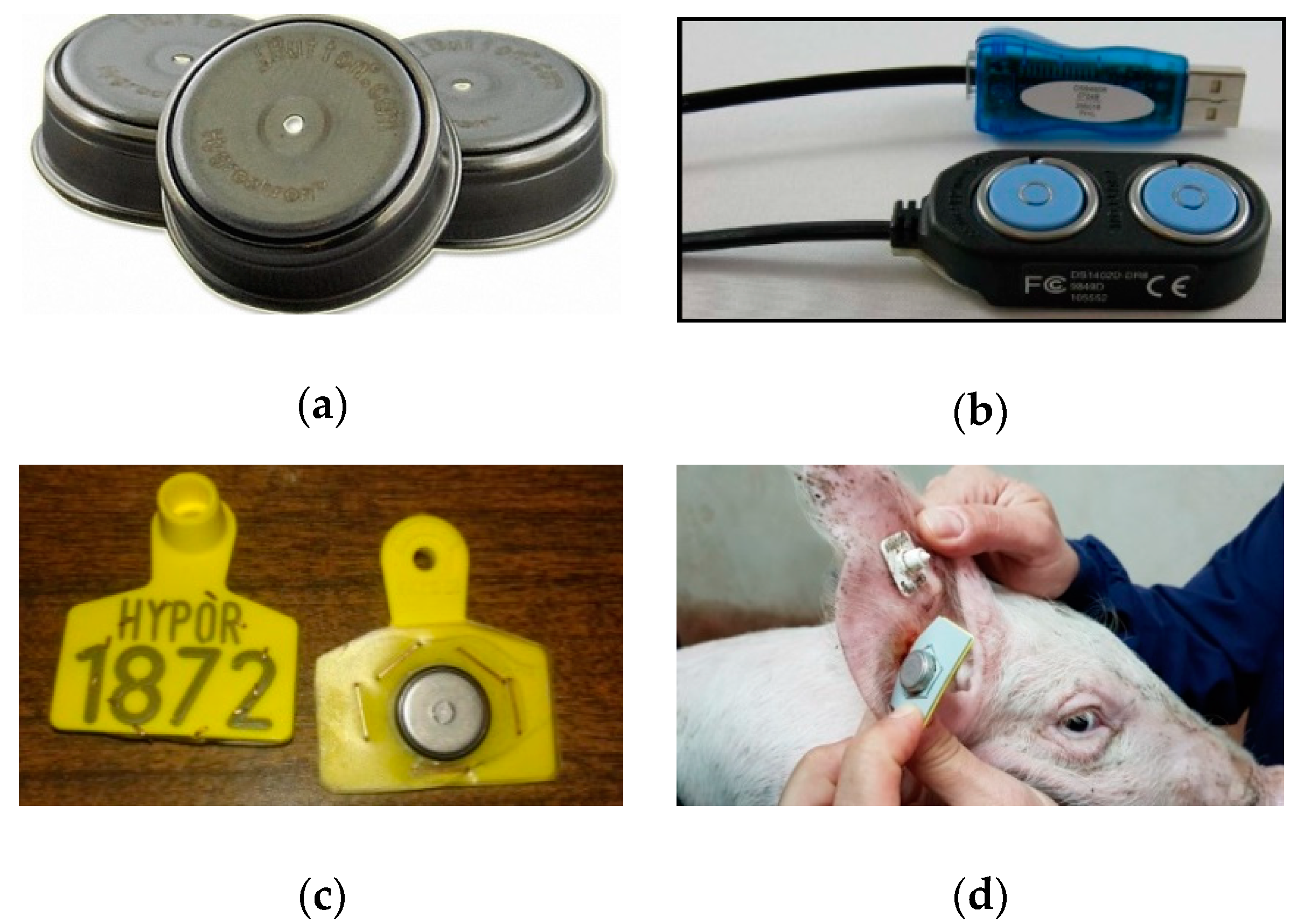
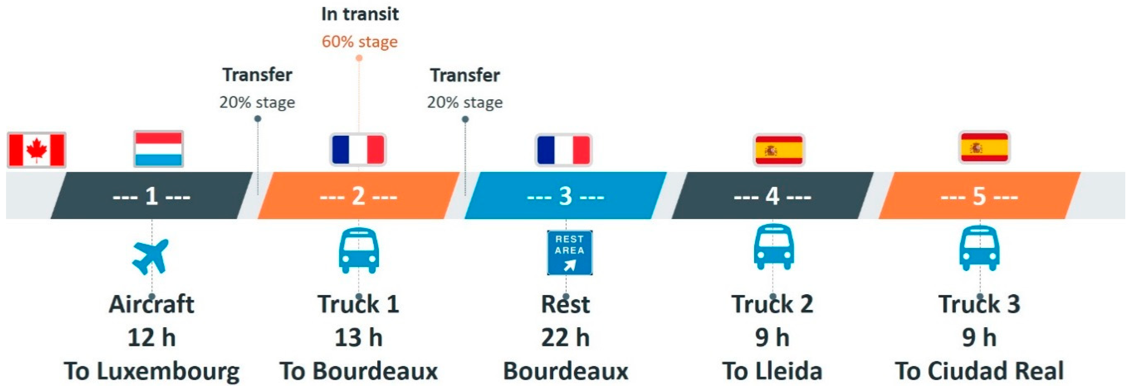
2. Materials and Methods

We monitored the EST of 11 Duroc pigs (7 females and 4 males, Table 1) during a 65 h commercial transport from a pathogen-free nucleus facility in Canada to Ciudad Real, Spain, from 19 to 22 May, 2016. The pigs were 46 to 114 days old, grouped into four classes: Group 1 nearly, 7 weeks old (3 animals, all of them females); Group 2, 10 weeks old (2 females); Group 3, 13 weeks old (3 animals, one male); and Group 4, 16 weeks old (3 males) (Table 1). Since the study was undertaken in commercial conditions, we were not allowed access to the animals during transport and were not able to weigh them before the journey. The journey was separated into five stages differentiated by vehicles used: Stage1-Air, aircraft travel from Toronto Airport to Luxembourg Airport (12 h); Stage2-Road, road transport from Luxembourg Airport to Bordeaux (13 h); Stage3-Rest, a rest period in Bordeaux (24 h); Stage4-Road, road transport from Bordeaux to Lerida (9 h); and Stage5-Road, road transport from Lerida to Ciudad Real (9 h).
Plane transport followed International Air Transport Association (IATA) Live Animals Regulations guidelines: using containers to ensure adequate ventilation of pigs and controlling environmental factors (standard recommendations for pigs over 7 kg 10–23.8 °C temperature, 0–75% RH and 0–3% for CO2) [24]. Each pig was housed individually in stalls with a litter of wood pellets and access to feed and water throughout the flight. Road transport was carried out in accordance with European Regulations for the protection of animals during transport [25]. The trailers used were 16 m long with two decks but no controlled environment system. The dimensions of the stall were 3 m long and 2.4 m in width and height. The pen floors had shavings and straw depending on the weather at the time of loading, and the animals fed during travel.
To measure EST, we used iButtons (DS1923, Maxim Integrated Product, Dallas, USA) (Figure 1a) with a resolution of 0.5 °C and a reported accuracy of ±0.5 °C. The loggers were launched before the journey began and downloaded after the last stage, using One Wire Viewer software (version 3.17.44; Figure 1b). Each iButton was fastened to the ID tag on the ear of each animal (Figure 1c) in such a way that it was in contact with the inner part of the ear (Figure 1d). Temperature was measured every 180 s (as in [18]), producing 1300 data points for the whole journey per animal.
To avoid considering EST values that corresponded to transfer times between different transport stages, we only considered 60% of the data, eliminating 20% of the data at the beginning and end of each stage (Figure 2). The averages and standard deviations (SD) of the EST were calculated per animal, per sex, and per journey stage. A one-way ANOVA analysis was performed considering stages as a factor. A one-way ANOVA and multiple comparison tests with Tukey’s honestly significant difference procedure were used to identify significant differences among the animals. MATLAB software (MATLAB R2015b, MathWorks, Inc., Natick, MA, USA) was used.

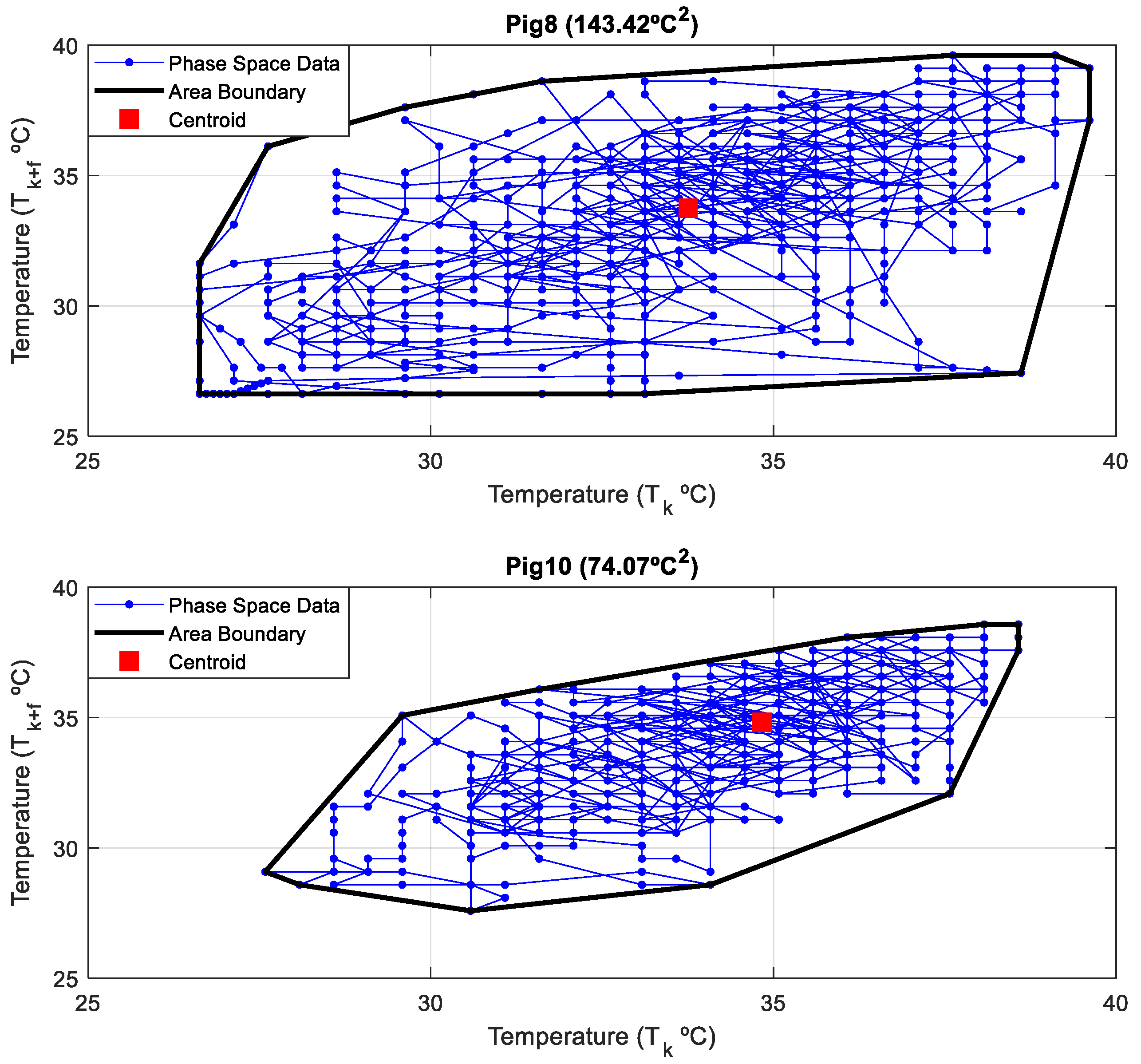
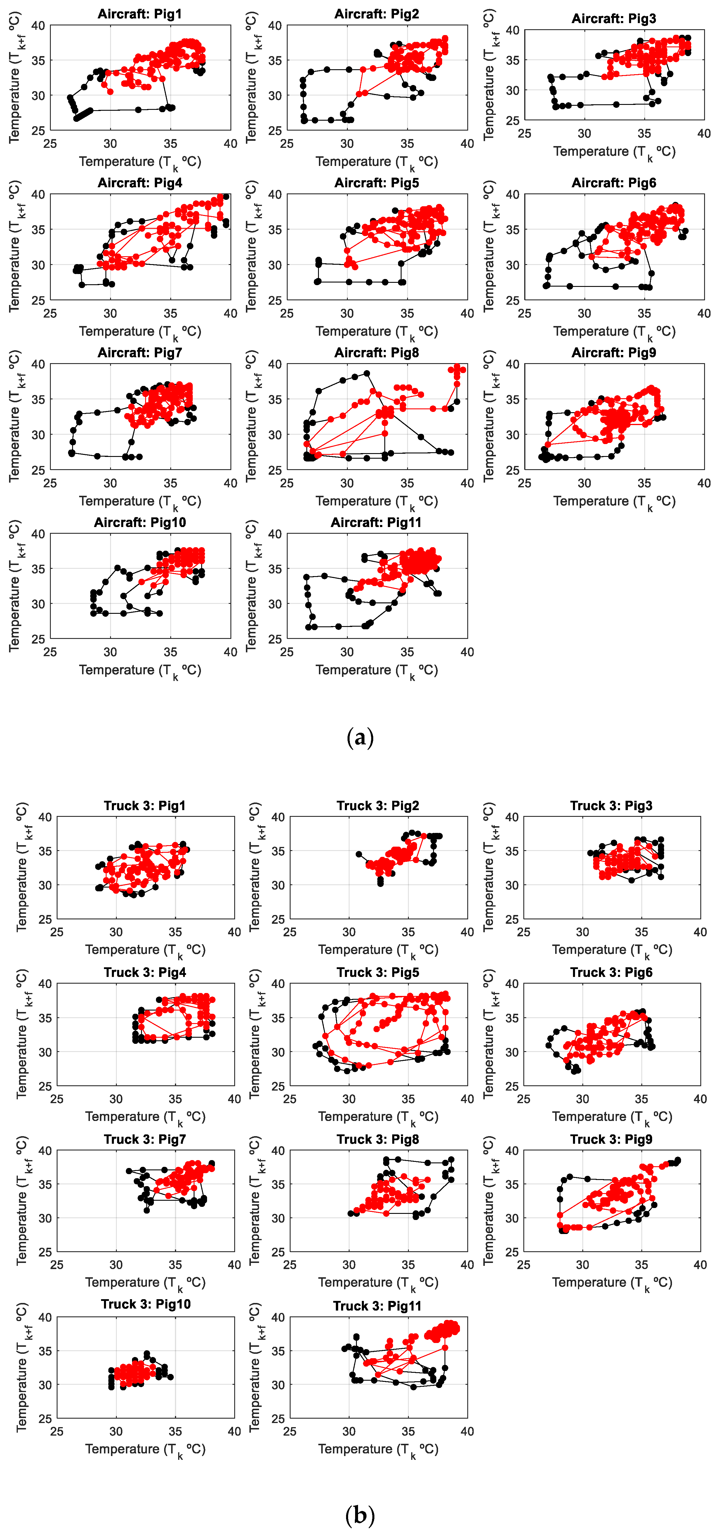
Phase Space Diagrams

Phase space diagrams were constructed for each pig based on the EST data, using time delays as in [26]. As explained in [19], each phase space was reconstructed in a phase space graph using a time series versus itself delayed in time. The appropriate value for the time delays (td) and system dimension (N) was obtained by heuristics. In this work, the two-dimensional (N = 2) space representations were obtained by plotting the measured temperature T(k) at each time t(k) versus the temperature T(k + ∆) at time t(k + ∆), with an optimum step ∆ (five in this work) established by heuristics. The data acquisition interval (i.e., the fixed time step of the time series) was τ min (3 min in this experiment), making the corresponding time delay td = τ·∆ = 15 min. Hahn et al. (1992) established that sampling intervals between 5 and 12.5 min are adequate from a biologically-based point of view in characterizing responses for tympanic temperature. In the current study, to obtain the optimum time delay of 15 min, different values of ∆ were tested systematically looking for the maximum expansion of the trajectory loops or attractors in the phase space, retaining the points that could represent specific events. The area of the trajectory loops was computed using the MATLAB functions (MATLAB R2015b, MathWorks, Inc., Natick, MA, USA) convhull and polyarea. The convhull function helps select a set of points from the trajectory loop in the phase space plot and returns the smallest convex envelope containing the set of points (vertices that define the polygon). The convhull function is based on the Quickhull (Qhull) algorithm for convex hulls. The polyarea function returns the area of vertices defined by convhull [19].
From these phase space diagrams, two variables of interest were extracted: (1) the centroid or center of gravity (°C) of the cloud of points that represent the arithmetic average of all ESTs registered, weighted by the local density of points or specific weight; and (2) the areas (°C2) that include all the points in the phase space as a measure of the total variability in EST during the selected periods, i.e., total area for the whole journey as well as for each stage. Since [27] showed how a phase space of time series can be useful to point out intense but short events, we calculated the area described by 100% of the points, as well as 75% of the points around the centroid. That helped us to identify any unique events in 25% of points furthest away from the centroid.

3. Results and Discussion

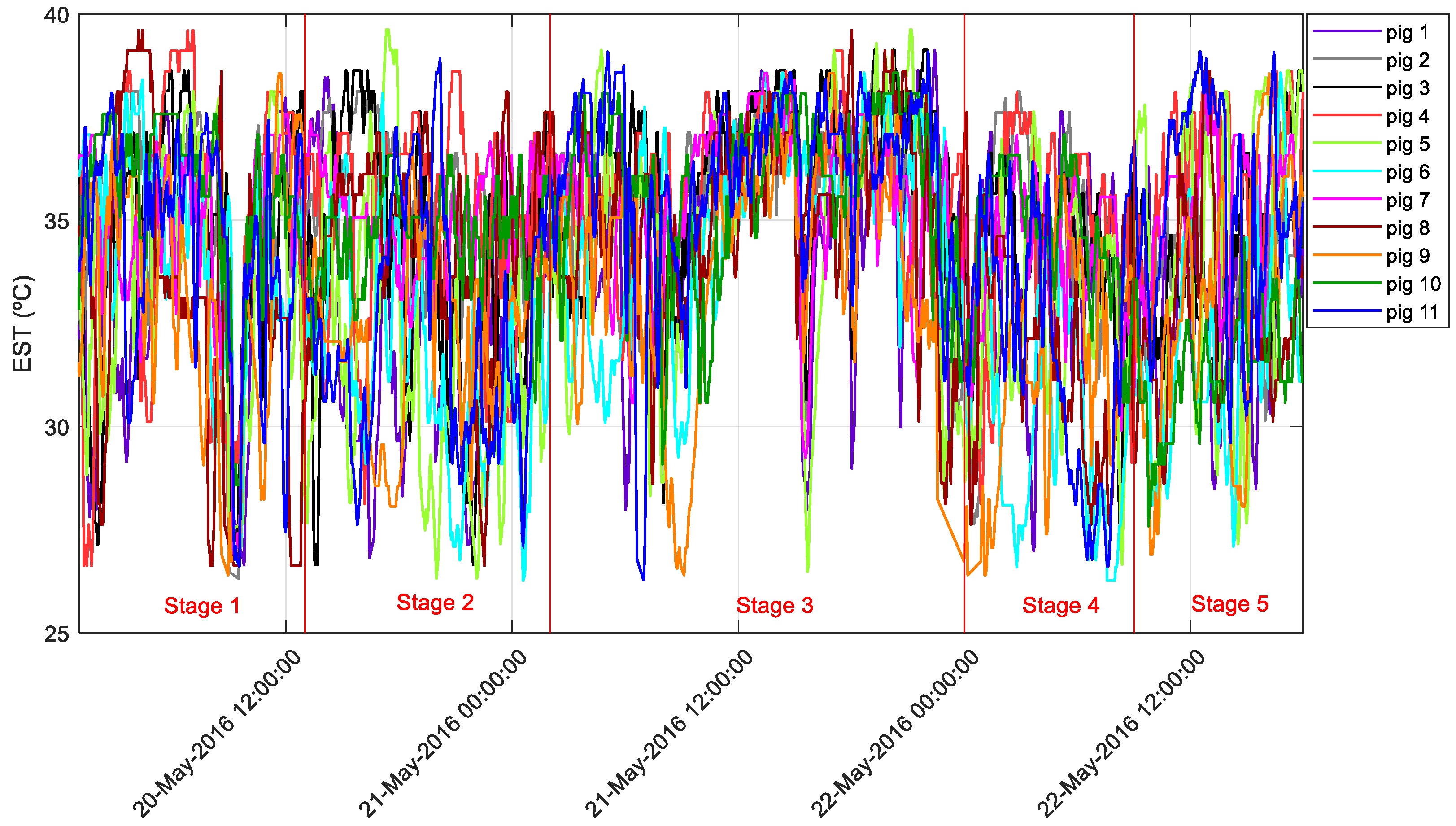
3.1. Pig Skin Temperature

Figure 3 shows the EST time series for the 11 pigs throughout the journey (65 h of transport). Vertical lines indicate the beginning and end of each transport stage. The instantaneous average EST ranged between 27.33 °C and 37.84 °C throughout the journey. The maximum difference among individuals was 12.26 °C during Stage2-Road, while the minimum difference was 0.66 °C during Stage3-Rest. There were no significant differences in average ESTs among animals (Figure 4) nor between Stage1-Air and other stages of road transport. Lewis [9] reported a wider variability with the average EST of piglets during road transport, ranging from 36.2 °C in summer to 23.1 °C in winter. Although we have not found studies that measure the EST in adult pigs continuously during road transport, Rocha et al. [28] report average skin temperatures of 30.89–36.02 °C, measured using thermography, which is similar to our results. The relationship between the surface temperature determined by thermography and the skin temperature determined by probes in contact with the animal has been reported before [29], in which the emissivity is calculated based on the assumption that both temperature measurements are similar.

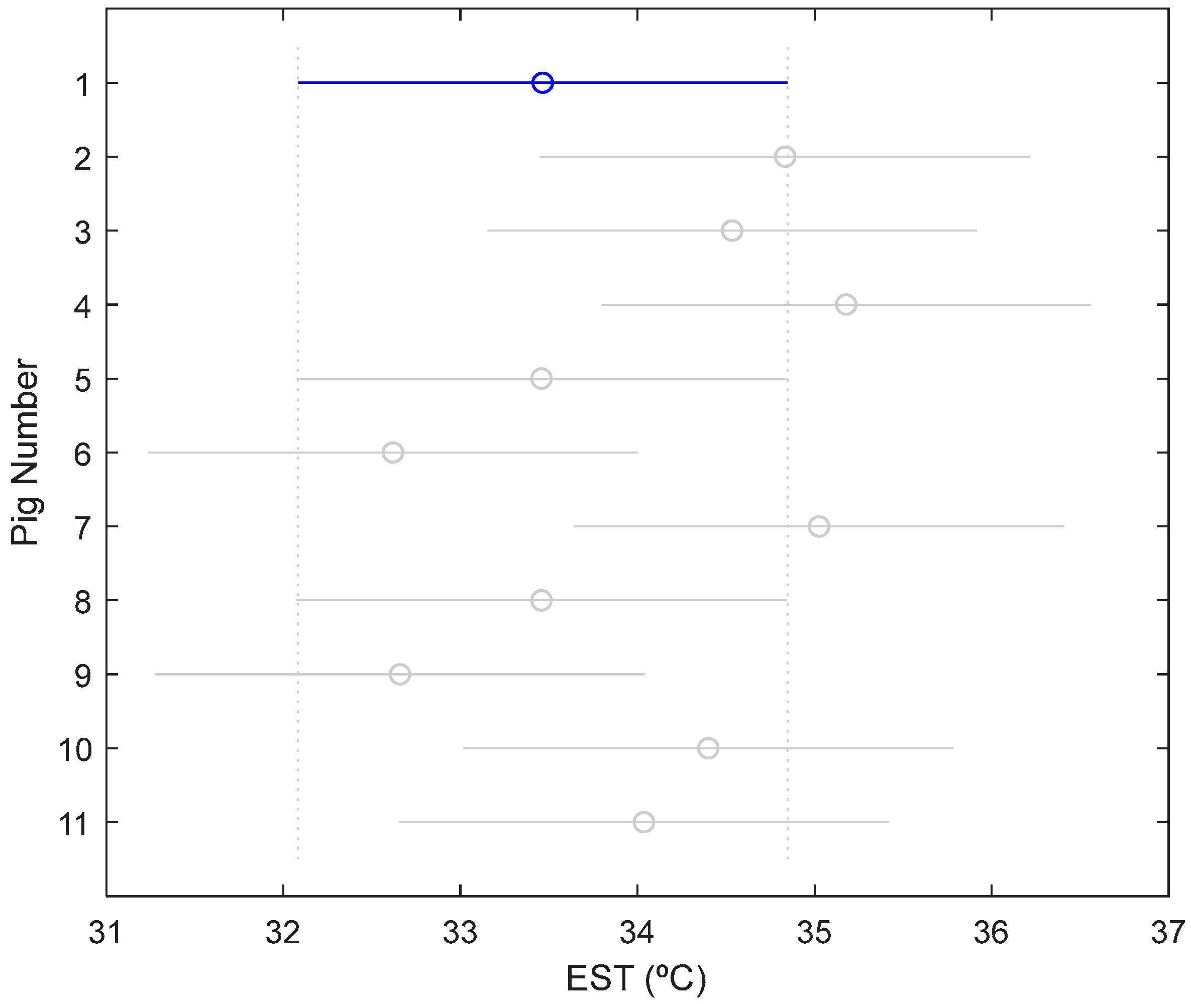
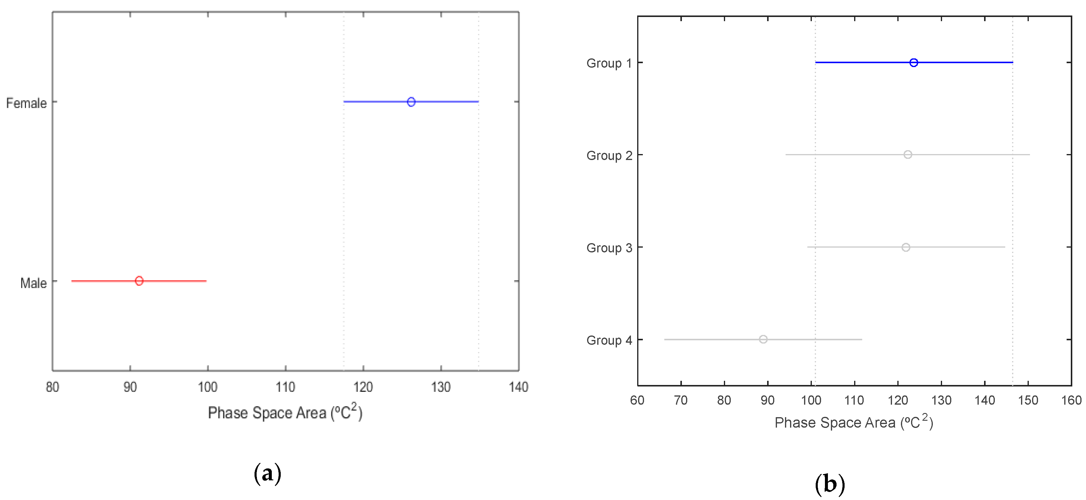
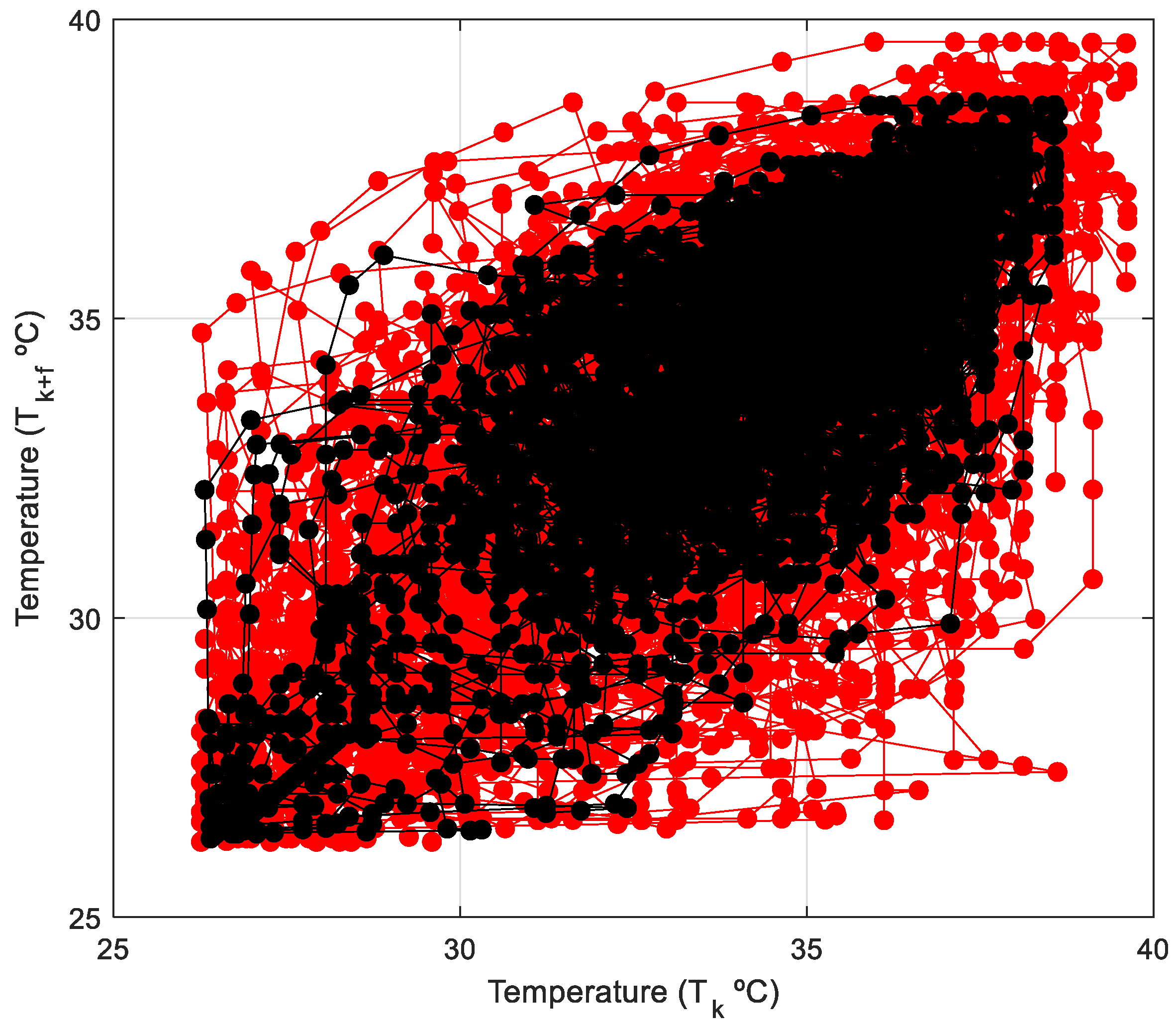
3.2. Phase Space: Variability in Skin Temperature by Animals

Table 2 summarizes the areas and centroids of the phase space diagrams per animal, considering the whole journey and different sex and age groups. The centroid value ranged from 32.8 °C to 35.1 °C, values of EST that are in accordance which those reported by Andersen et al. [18] in adult commercial crossbreed pigs. The maximum area corresponded with Pig 8 (Figure 5), a female belonging to age Group 3 (143.4 °C2). The minimum area was for Pig 10, a male belonging to age Group 4 (74.1 °C2). There were significant differences between sexes (F = 20.81, p = 0.0014, Figure 6a), with areas being around 30% higher in females (Figure 7). Nonetheless, the significance level of the difference among age groups (based on the analysis of variance) was only 10% (F = 2.94, p = 0.10, Figure 6b), separating Group 4 (all males) from the rest. Larger animals had a higher average EST and lower phase space area, which suggests that their thermal variability was lower. This could be due to the higher metabolic heat production and the decreasing surface area to mass ratio as animals grow [21,30]. In order to provide visualization, the EST phase space for a male and a female pig are shown in Figure 5, with a time delay of 15 min (td = 15 min).

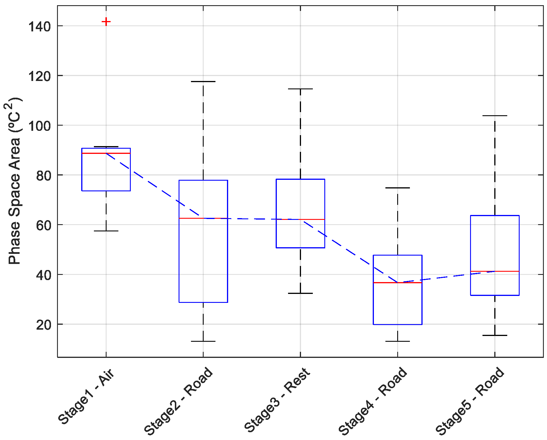
3.3. Phase Space: Variability in EST by Transport Stage

Table 3 summarizes the areas and centroids of the phase space diagrams per animal per transport stage. The highest centroids (34.1 °C and 35.5 °C) corresponded with Stage1-Air and Stage3-Rest, while all road transport stages had centroids close to 33.5 °C. Stage1-Air and Stage3-Rest had the highest average areas in the phase space (85.7 and 67.1 °C2, respectively). The average area in Stage3-Rest was 22% lower than Stage1-Air, while the duration of the Stage3-Rest was almost double that of Stage1-Air. Thus, we can use the area of the phase space diagrams to compare the thermal variability among stages of different duration, where the value of the area was not correlated with the duration of the times series considered. During road transport (Stages 2 to 5), the thermal variability in terms of areas was between 67% and 43% lower than Stage1-Air.
In Figure 8, we show the medians and the interquartile ranges of the areas of the phase space diagrams per transport stage. Stage1-Air had the highest median with the lowest interquartile range, which indicates the variation in EST was the highest and also similar among all pigs. On the other extreme, Stage2-Road had the highest interquartile range, indicating that EST varied differently among pigs, with some being quite stable (e.g., Pig 10 with 13.1 °C2), while others were more variable (e.g., Pig 5 with 117.6 °C2). These results could be related to the position of the pigs on the vehicle since it has been shown that position affects the micro-environment in each pen and, as a result, also the skin temperature of the animals [15]. According to the ANOVA, there were significant differences among the areas for Stage1-Air compared with the road transport stages (F = 6.4, p = 0.0003).
To elucidate the reasons for the greater thermal variability during air travel, we have represented the phase space diagrams per animal during air travel and during one of the stages of road transport. From the representation of the complete time series in the phase space diagram, we identified different dynamics, some with a more homogeneous distribution and concentration of points in the whole area within the envelope, and others where the points are more dispersed. Figure 9 shows the phase space diagram corresponding with Stage1-Air (heterogeneous distribution of points) and Stage5-Road for all animals (homogeneous distribution of points, especially for Pigs 1, 3, and 10); red dots are 75% of the points closest to the centroid. The spatial concentration of 75% of the dots in a very small area implies it is an attractor that all pigs tend toward. In the case of Stage1-Air, black dots (25% of the data furthest from the centroid) were more dispersed and further from the attractor. Thus, they can be interpreted as a representation of a specific and unique event, which caused an average increase in the area of 62% when shifting from considering 75% to 100% of the dots (Figure 9a). That event lasted 57 min, leading to a general decrease in EST by 8 °C with respect to the average value of the centroid (34.1 °C). We did not find a similar or generalized phenomenon (i.e., that affected all animals) in the rest of the transport stages. The same analysis carried out in the road transport stages caused an average increase in the area from 49.5% when going from considering 75% to 100% of the points (Figure 9b), showing that both the event number and its effect on the thermal variability was much higher during air transport compared with road transport. Previous work by other authors has shown that the visualization using phase spaces allows easy identification of events such as the opening of a door in cold rooms or when refrigeration equipment is turned on or off [27]. The event detected in Stage1-Air, with an abrupt decrease in temperature that affected all the animals, could be explained by a local change in parameters of air-conditioning.

4. Conclusions

We were able to successfully record individual EST of pigs over a 65 h journey in a non-invasive manner, including air travel and road transport. The basal values obtained are similar to previous studies using other technologies such as thermal images or infrared radiometers. The area of the centroid of the phase space diagram (which quantifies variability) is an objective variable that characterizes the dynamics of the EST during each stage of the journey and is the most informative variable. The phase space representation of the EST time series allowed us to differentiate among male and female pigs, based on older animals (F = 20.81, p = 0.0014), where thermal stability was higher in males. That greater stability could be since skin temperature is influenced by metabolic heat production and the surface area to mass ratio, which are higher and lower, respectively, in heavier animals. The area of the phase space diagrams was highest during Stage1-Air, indicating that EST was more variable than the rest of the stages, almost double that of road stages. This methodology allowed us to compare thermal variability independently of the duration of each stage. In Stage1-Air, the increase in the area was more than 60% when including 75% to 100% of the points, thereby allowing to identify an event close to a one-hour duration and generalized among all animals. The use of the phase space diagram has shown to be useful to tease out new information from the temperature time series, facilitating the detection of events and the identification of thermal dynamics of the different types of animals. The instrumentation and methodology used in this article could help to build a new tool that could be used during multimodal commercial transport to complement other possible stress indicators. For that, it would be necessary to carry out further work in which the logging of EST data is complemented with other stress indicators and other information on the environmental and management conditions.

Author Contributions

Conceptualization B.D., M.G.-I., and J.-M.R.; methodology, investigation, and formal analysis, B.D., E.-C.C., and M.G.-I.; software development and data curation, M.G.-I.; writing—original draft preparation, M.G.-I., B.D., and E.-C.C.; writing—review and editing, M.V.; visualization, B.D., E.-C.C., and M.V.; supervision and project administration, B.D.; funding acquisition and resources, B.D. and J.-M.R.

Funding

This research was funded by the Ministerio de Economía, Industria y Competitividad and the Agencia Estatal de Investigación of Spain through PRINCE. RTC-2017-5977-2 project.

Conflicts of Interest

The authors declare no conflicts of interest.

References

  1. Ritter, M.; Ellis, M.; Berry, N.; Curtis, S.; Anil, L.; Berg, E.; Benjamin, M.; Butler, D.; Dewey, C.; Driessen, B. Transport losses in market weight pigs: I. A review of definitions, incidence, and economic impact. Prof. Anim. Sci. 2009, 25, 404–414. [Google Scholar] [CrossRef] [Green Version]
  2. Comission, E. Guide to good practices for the transport of pigs. In Consortium of the Animal Transport Guides Project (2017-rev1); Revision May 2018; European Commission: Brussels, Belgium, 2018. [Google Scholar]
  3. Bench, C.; Schaefer, A.; Faucitano, L. The welfare of pigs during transport. In Welfare of Pigs: From Birth to Slaughter; Schaefer, A., Faucitano, L., Eds.; Wageningen Academic: New York, NY, USA, 2008; Volume 6, pp. 161–180. [Google Scholar]
  4. Faucitano, L.; Rioja-Lang, F.C.; Brown, J.A.; Brockhoff, E.J. A review of swine transportation research on priority welfare issues: A canadian perspective. Front. Vet. Sci. 2019, 6, 36. [Google Scholar]
  5. Lambooij, E. Transport of pigs. Livest. Handl. Transp. 2014, 1, 280–297. [Google Scholar]
  6. Grandin, T. Safe handling of large animals: Part II. Ir. Vet. J. 2008, 61, 758–763. [Google Scholar]
  7. Roldan-Santiago, P.; Martinez-Rodriguez, R.; Yanez-Pizana, A.; Trujillo-Ortega, M.E.; Sanchez-Hernandez, M.; Perez-Pedraza, E.; Mota-Rojas, D. Stressor factors in the transport of weaned piglets: A review. Vet. Med. 2013, 58, 241–251. [Google Scholar] [CrossRef] [Green Version]
  8. Villarroel, M.; Barreiro, P.; Kettlewell, P.; Farish, M.; Mitchell, M. Time derivatives in air temperature and enthalpy as non-invasive welfare indicators during long distance animal transport. Biosyst. Eng. 2011, 110, 253–260. [Google Scholar] [CrossRef]
  9. Lewis, N.J. Transport of early weaned piglets. Appl. Anim. Behav. Sci. 2008, 110, 128–135. [Google Scholar] [CrossRef]
  10. Sommavilla, R.; Faucitano, L.; Gonyou, H.; Seddon, Y.; Bergeron, R.; Widowski, T.; Crowe, T.; Connor, L.; Scheeren, M.; Goumon, S. Season, Transport Duration and Trailer Compartment Effects on Blood Stress Indicators in Pigs: Relationship to Environmental, Behavioral and Other Physiological Factors, and Pork Quality Traits. Animals 2017, 7, 8. [Google Scholar] [CrossRef]
  11. Lewis, M.C.; Inman, C.F.; Patel, D.; Schmidt, B.; Mulder, I.; Miller, B.; Gill Bhupinder, P.; Pluske, J.; Kelly, D.; Stokes, C.R. Direct experimental evidence that early-life farm environment influences regulation of immune responses. Pediatr. Allergy Immunol. 2012, 23, 265–269. [Google Scholar] [CrossRef]
  12. Brown, S.; Knowles, T.; Wilkins, L.; Chadd, S.; Warriss, P. The response of pigs to being loaded or unloaded onto commercial animal transporters using three systems. Vet. J. 2005, 170, 91–100. [Google Scholar] [CrossRef]
  13. Mayer, J.J.; Davis, J.D.; Purswell, J.L.; Koury, E.J.; Younan, N.H.; Larson, J.E.; Brown-Brandl, T.M. Development and characterization of a continuous tympanic temperature logging (CTTL) probe for bovine animals. Trans. ASABE 2016, 59, 703–714. [Google Scholar]
  14. Chen, C.-S.; Chen, W.-C. Research and Development of Automatic Monitoring System for Livestock Farms. Appl. Sci. 2019, 9, 1132. [Google Scholar] [CrossRef] [Green Version]
  15. Xiong, Y.; Green, A.; Gates, R. Characteristics of trailer thermal environment during commercial swine transport managed under US industry guidelines. Animals 2015, 5, 226–244. [Google Scholar] [CrossRef] [PubMed]
  16. Stiehler, T.; Heuwieser, W.; Pfützner, A.; Burfeind, O. The course of rectal and vaginal temperature in early postpartum sows. J. Swine Health Prod. 2015, 23, 72–83. [Google Scholar]
  17. Wiersma, F.; Stott, G.H. A technique for securing a temperature probe adjacent to the tympanic membrane in bovine. Trans. ASAE 1983, 26, 185–0187. [Google Scholar] [CrossRef]
  18. Andersen, H.M.-L.; Jørgensen, E.; Dybkjær, L.; Jørgensen, B. The ear skin temperature as an indicator of the thermal comfort of pigs. Appl. Anim. Behav. Sci. 2008, 113, 43–56. [Google Scholar] [CrossRef]
  19. Requejo, J.M.; Garrido-Izard, M.; Correa, E.C.; Villarroel, M.; Diezma, B. Pig ear skin temperature and feed efficiency: Using the phase space to estimate thermoregulatory effort. Biosyst. Eng. 2018, 174, 80–88. [Google Scholar] [CrossRef] [Green Version]
  20. Sellier, N.; Guettier, E.; Staub, C. A review of methods to measure animal body temperature in precision farming. Am. J. Agric. Sci. Technol. 2014, 2, 74–99. [Google Scholar] [CrossRef]
  21. Mayorga, E.J.; Renaudeau, D.; Ramirez, B.C.; Ross, J.W.; Baumgard, L.H. Heat stress adaptations in pigs. Anim. Front. 2019, 9, 54–61. [Google Scholar] [CrossRef]
  22. Hahn, G.; Chen, Y.; Nienaber, J.; Eigenberg, R.; Parkhurst, A. Characterizing animal stress through fractal analysis of thermoregulatory responses. J. Therm. Biol. 1992, 17, 115–120. [Google Scholar] [CrossRef]
  23. Korthals, R.; Eigenberg, R.; Hahn, G.; Nienaber, J. Measurements and spectral analysis of tympanic temperature regulation in swine. Trans. ASAE 1995, 38, 905–909. [Google Scholar] [CrossRef]
  24. IATA. International Air Transport Association Live Animals Regulations; IATA: Geneva, Switzerland, 2001. [Google Scholar]
  25. EC. European Council. No 1/2005 of 22 December 2004 on the protection of animals during transport and related operations and amending Directives 64/432/EEC and 93/119/EC and Regulation (EC) No 1255/97. Off. J. Eur. Union 2005, 3, 1–44. [Google Scholar]
  26. Eckmann, J.-P.; Ruelle, D. Ergodic theory of chaos and strange attractors. In The Theory of Chaotic Attractors; Springer: Berlin/Heidelberg, Germany, 1985; pp. 273–312. [Google Scholar]
  27. Jiménez-Ariza, T.; Correa, E.; Diezma, B.; Silveira, A.C.; Zócalo, P.; Arranz, F.J.; Moya-González, A.; Garrido-Izard, M.; Barreiro, P.; Ruiz-Altisent, M. The phase space as a new representation of the dynamical behaviour of temperature and enthalpy in a reefer monitored with a multidistributed sensors network. Food Bioprocess Technol. 2014, 7, 1793–1806. [Google Scholar] [CrossRef] [Green Version]
  28. Rocha, L.M.; Devillers, N.; Maldague, X.; Kabemba, F.Z.; Fleuret, J.; Guay, F.; Faucitano, L. Validation of Anatomical Sites for the Measurement of Infrared Body Surface Temperature Variation in Response to Handling and Transport. Animals 2019, 9, 425. [Google Scholar] [CrossRef] [PubMed] [Green Version]
  29. Soerensen, D.D.; Clausen, S.; Mercer, J.B.; Pedersen, L.J. Determining the emissivity of pig skin for accurate infrared thermography. Comput. Electron. Agric. 2014, 109, 52–58. [Google Scholar] [CrossRef]
  30. Poczopko, P. Metabolic rate and body size relationships in adult and growing homeotherms. Acta Theriol. 1979, 24, 125–136. [Google Scholar] [CrossRef]
Figure 1. (a) iButton Loggers DS1992 E. (b) Desktop reader for iButton DS1402D-DR8. (c) Detail of the iButton sensor coupling to the tag. (d) Installation of the sensor with the sensor attached to the animal to be monitored.
Applsci 09 05527 g001
Figure 2. Full journey outline from Stages 1 to 5 with indication of the characteristics of each stage.
Applsci 09 05527 g002
Figure 3. Time series of ear skin temperatures (EST).
Applsci 09 05527 g003
Figure 4. Summary of the mean EST per pig over the whole journey. The mean EST of each pig is represented by a circle, and the interval is represented by a line extending from the symbol. The highlighted Pig Number 1 (in blue) is not significantly different from the rest of the animals (in gray).
Applsci 09 05527 g004
Figure 5. Phase space representation of EST for Pigs 8 (female, Group 3) and 10 (male, Group 4) throughout the journey (f = 5).
Applsci 09 05527 g005
Figure 6. Results from the multiple comparison of group mean phase space areas. Each group (a): sex; (b): age group mean is represented by a circle, and the interval is represented by a line extending out from the symbol. Red color indicates it is significantly different from the blue one (p < 0.05), while gray color indicates no significant differences with the highlighted group (in blue).
Applsci 09 05527 g006
Figure 7. Phase space representation for all data (whole trip) of male pigs (black) and female pigs (red), (f = 5).
Applsci 09 05527 g007
Figure 8. Boxplot of the areas obtained by using a phase space representation for each stage. Central mark indicates the median, and the bottom and top edges of the box indicate the 25th and 75th percentiles, respectively. The whiskers that extend to the most extreme data points are not considered outliers, and the outliers are plotted individually using the ‘+’ symbol.
Applsci 09 05527 g008
Figure 9. Phase space representation by considering 100% (black) or 75% (red) of the points furthest from the centroid during: (a) Stage1-Air and (b) Stage5-Road for each monitored pig (f = 5).
Applsci 09 05527 g009
Table 1. Summary of the pigs used in the study including sex, birth date, age group, and weight upon arrival (see text).
Pig NumberSexBirth DateAge GroupWeight (kg)
1Female04/04/2016115.38
2Male30/01/2016478.47
3Female04/04/2016118.19
4Female18/02/2016349.48
5Female02/04/2016117.41
6Female11/03/2016230.65
7Male18/02/2016345.22
8Female17/02/2016348.5
9Male30/01/2016458.51
10Male27/01/2016485.64
11Female10/03/2016228.93
Table 2. Summary of EST centroid value and area obtained using the phase space representation.
Pig NumberArea (°C2)Centroid (°C)
1121.633.7
293.435.0
3111.334.8
4124.235.3
5138.233.6
6111.633.1
797.935.1
8143.433.8
999.132.8
1074.134.8
11132.834.3
Mean113.434.2
Table 3. Areas and centroids obtained using the phase space representation for each transport stage and pig (C = centroid temperature; STD = standard deviation).
Stage1-AirStage2-Road Stage3-RestStage4-Road Stage5-Road
Area (°C2)C (°C)Area (°C2)C (°C)Area (°C2)C (°C)Area (°C2)C (°C)Area (°C2)C (°C)
Pig 174.433.448.331.080.635.274.833.741.232.4
Pig 289.034.422.235.641.735.725.335.529.834.2
Pig 390.534.982.433.970.336.313.734.729.833.6
Pig 488.734.462.635.432.436.427.435.937.135.7
Pig 578.034.1117.631.696.734.941.833.3103.933.9
Pig 690.834.464.131.158.335.448.430.249.031.8
Pig 773.333.914.534.762.135.917.934.736.935.7
Pig 8141.733.578.634.161.635.336.732.051.733.5
Pig 967.732.256.031.971.234.145.932.468.732.8
Pig 1057.535.413.134.848.135.613.135.415.531.6
Pig 1191.434.275.832.9114.635.854.931.667.635.9
Mean85.734.157.733.467.135.536.433.648.333.7
STD21.70.832.01.723.80.719.21.924.41.5

