Abstract
In this paper, case studies were carried out to analyze the feasibility of submerged floating tunnels (SFTs) with suspension cables. In order to apply an SFT in a field site, the deformation of the system should be controlled, even under extreme wave conditions, if vehicles or trains operate inside the SFT. Two types of suspended SFTs were proposed to analyze their hydrodynamic behavior. The main variables were the wave conditions, cross-sectional diameters, buoyancy weight ratios, inclination angles of the main cables, and installation depth of the SFT. Overall, it was found that the SFT with a mid-anchor was superior from a hydrodynamic point of view. However, a detailed hydrodynamic analysis must be performed to avoid the conditions that previously produced slack. In addition, in a case where acceleration is generated by motion, the design should be reviewed to ensure safe conditions, according to the traffic passage.
1. Introduction
Submerged floating tunnels (SFTs) float underwater and have an innovative water-crossing typology, supported by Archimedes’ principle [1]. While SFTs are placed underwater, they differ from the conventional immersed tunnels, which are placed directly on the seabed and are composed of segments. However, they have several structural or infrastructural issues. Several proposals for SFTs have been designed by different countries, after the concept was proposed by Sir Edward James Reed of the United Kingdom in 1886, and are continuously being studied in the United States, France, Norway, Japan, Italy, Canada, Switzerland, Korea, China, and so forth. An SFT has its own weight and buoyancy, according to its immersion depth volume. Generally, the tunnel cross section is designed so that the buoyancy covers the structural weight, and the tunnel is then subjected to an upward force, which is exerted by a fluid [2]. Based on the vertical support, the current design alternatives for SFTs can be divided into two categories, as shown in Figure 1: a tether stabilized concept (Figure 1a) and a pontoon-stabilized concept (Figure 1b).
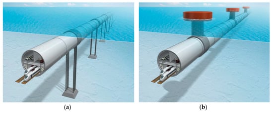
Figure 1.
Basic concept of submerged floating tunnels (SFTs): (a) tether-stabilized submerged floating tunnel concept; (b) pontoon-stabilized submerged floating tunnel concept.
In particular, Italy has been continuing its research on SFTs, as an alternative to crossing the straits, since the 1960s. Norway have advanced SFT technologies. The SIJLAB (Sino-Italian Joint Laboratory of Archimedes’ Bridge) [3], as a Sino-Italian joint venture, was founded in 1998 and was co-financed by the Institute of Mechanics, Chinese Academy of Sciences, China and the “Ponte di Archimede International” company. The consortium has carried out the executive design of a prototype tunnel, with a length of 100 m, in Qiandao Lake in the eastern province of Zhejiang, China [3]. In addition, Norway is working on the world’s first SFT project to cross the fjords. It is a long journey between Kristiansand and Trondheim, which is part of the E39 route, crossing the southwestern coast. The Norwegian Public Roads Administration (NPRA) aims to complete the construction by 2050 and plans to cut travel time by half [4]. However, this project focuses mainly on core technology research concerning a preliminary design and lacks experience in the practical application of an SFT, which involves, for instance, design standards and economic evaluation, and the tunnel has never been built (as of 2018). Lin et al. (2019) [5] conducted an investigation on the vehicle–tunnel coupled vibration of SFT using tether vibration, and the Hamilton principle and D’Alembert’s principle were used to define a theoretical model. Xiaing and Yang (2017) [6] researched the global dynamic performance of a submerged floating tunnel (SFT) under an impact load. Seo et al. (2015) [7] presented a theoretical method, and tests using experimental models involving a wave were proposed for verification. Xiang et al. (2018) [8] studied the global dynamic response of an SFT under anchor-cable failure, considering the post-breakage performance. Lu et al. (2011) [9] studied the dynamics of an SFT, when its behavior was affected by tether slack and snap force under wave conditions. Jin and Kim [10] studied time-domain hydro-elastic analysis of SFT using an finite element model under extreme wave and seismic excitations. Chen et al. [11] researched coupled vibration performance of SFT in wave and current.
Won and Kim (2018) [12] proposed a concept design for an SFT with an inclined cable, as an application form. It is shown in Figure 2. The hydrodynamic characteristics of the SFT were studied, and a case study on the diameters, drafts, and BWR (buoyancy and weight ratio), as variables, was conducted. In this study, a feasibility study on the applicability of an SFT with suspension cables (Figure 3) was performed at an arbitrary site. Figure 4 illustrates two solutions concerning the components of SFTs with suspension cables, which consist of towers, main cables, hangers and anchorages. The tube, the main body an SFT, is suspended on a hanger rope and transmits a dead load and a live load, which are arranged at regular intervals, to a hanger. Moreover, they hang from the main cable, so that they can transfer the load of the SFT to the main cable. Unlike conventional suspension bridges, since the main cable of SFTs holds loads by buoyant forces uniformly, it can be the main generator of tension and control the behavior of the SFT. The tower is a supporting component, like the tube and main cables. The SFT with a tower differs from the SFT with inclined cables, shown in Figure 2, in that the hanger supports this system vertically, so that the compressive force does not act on the tube body.
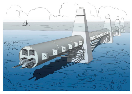
Figure 2.
Concept design of a submerged floating tunnel with inclined cables.
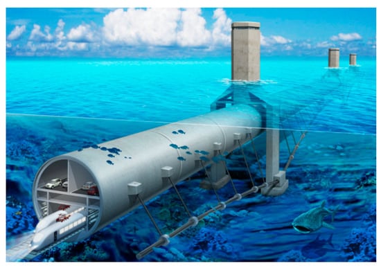
Figure 3.
Concept design of a submerged floating tunnel with suspension cables.
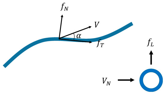
Figure 4.
Hydrodynamic force on a pipe or tendon.
In this paper, case studies were analyzed to determine the feasibility of an SFT with suspension cables. In order to apply the SFT in a field site, the deformation of the system should be controlled, even under extreme wave conditions if vehicles or trains operate inside the SFT. The main variables were set to be the diameter of the tube, layout methods and layout angles of the main cable, BWR (buoyancy and weight ratio), installation depths, and wave heights. The optimal conditions for the aforementioned variables were derived by analyzing the behavior of the SFT with suspension cables under irregular waves. Here, the installation depth required to minimize the effect of breaking waves and maritime activity is named the top clearance or the draft in offshore engineering.
2. Fluid–Structure Interaction Analysis of SFT under Waves
Governing Equation and Fluid Force of a Submerged Line Element
The governing differential equation of a pipe and a tendon for SFT-acting static loads, such as self-weight, buoyancy, and tidal current, was determined, and the dynamic load of waves can be constructed through DNV-RP-C205 [13].
The hydrodynamic force on a slender beam in a general fluid flow can be determined by adding up the sectional forces acting on each point of the beam structure as shown Figure 4. Generally, the force vector acting on a beam can be resolved into a normal force , a tangential force and a loft force , which is the same as both and . Additionally, a torsion moment will occur on non-circular cross-sections.
For slender structural beam members with a cross-sectional dimensions and insufficient planarity to allow the inclination of fluid velocities and the accelerations of particles in the normal flow direction to the beam member, to be neglected, the wave loads can be estimated using Morison’s load formula, which is the sum of an inertia force, proportional to the acceleration, and a drag force, which is proportional to the square of the velocity.
Normally, Morison’s load formula is used when the following condition is satisfied by Equation (1):
where is the wavelength, and is the diameter. When the beam member’s length is larger than the cross dimensions, the end-effects can be neglected, and the total force can be taken as the sum of forces on each cross-section area, according to the length of the beam. As for the wave and flow conditions, they induced particle velocities, which should be supplemented with vector quantities.
The sectional force on a fixed slender beam in a normal two-dimensional flow to the member axis is given by:
= the fluid particle (waves and/or current) velocity (m/s), = the fluid particle acceleration (2 ), = the cross sectional area (m2), D = the diameter or typical cross-sectional dimension (m), = the mass density of the fluid (2 ), = the added mass coefficient (with a cross-sectional area as a reference area), and = the drag coefficient.
The drag coefficient is the non-dimensional drag force:
where = the sectional drag force (N/m).
In general, the fluid velocity vector will be in a direction, relative to the axis of the slender member. The drag force is decomposed with a normal force and a tangential force .
The mass coefficient is defined as:
3. Global Performance of SFTs with Suspension Cables
In this section, a new concept of suspended SFT models, with two solutions, is suggested, as shown in Figure 5 and Figure 6. Figure 5a and Figure 6b display Type 1, which has towers on both ends and main cables connected to the towers. On the contrary, Type 2, shown in Figure 5b, has an additional anchorage in the middle of both towers. Figure 5b shows the dimensions of Type 1, which are based on anchorages at both towers, and a main cable that connects them and is supported by hangers between the main cable and the tube. In contrast, Figure 6c represents the dimensions of Type 2, in which a form of anchorage is installed at the required position, and the main cable is arranged so that it can control the displacement of the center between the towers effectively. To investigate the global performance of the SFT, the commercial finite element program, ABAQUS AQUA (SIMULIA, IA, USA), was used [14]. This program can consider various ocean environmental conditions, such as irregular waves, currents, etc.
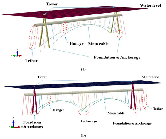
Figure 5.
Components of the submerged floating tunnel with suspension cables. Finite element model by ABAQUS [14]: (a) Type 1; (b) Type 2.
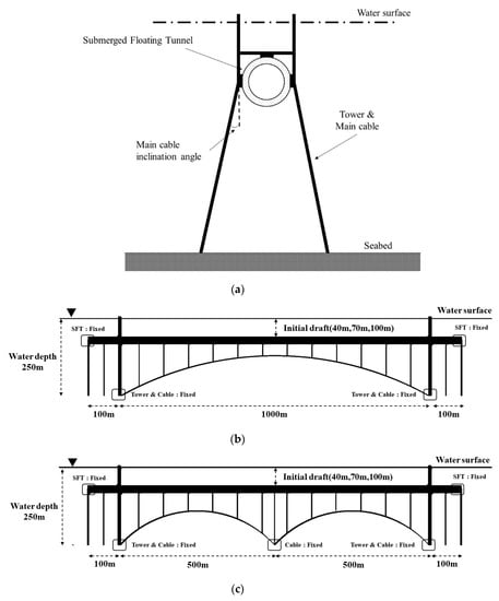
Figure 6.
Considered suspension SFT: (a) section view; (b) dimensions of Type 1; (c) dimensions of Type 2.
Furthermore, Figure 6a exhibits the variables of the analysis of the section view of the suspended SFT. It was assumed that both ends are fixed boundary conditions on land. The main span of Type 1 was 1000 m in length, and in Type 2, two arched main cables were installed at the middle anchorage. The towers and main cables were fixed at the anchorages. Moreover, hangers and tethers on the side of the main cables were hinged to the foundation.
The environmental conditions and specifications for the SFT model are shown in Table 1. To begin with, the conditions of the model were set as follows: A water depth of 280 m and significant wave heights (periods) of 3.5 m (5 s), 6.0 m (8 s), and 8.0 m (10 s). Moreover, the irregular waves in a time series, as shown in Figure 7, were applied using the JONSWAP spectrum. [15] The suspended SFT consists of a tube, main cables, hangers, towers and side tethers, as shown in Figure 5 and Figure 6.

Table 1.
Geometric and environmental conditions for the case study.
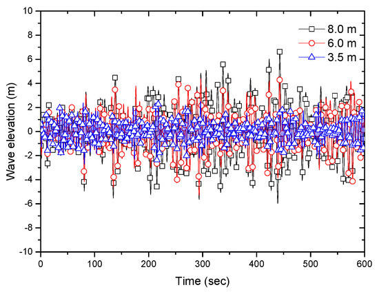
Figure 7.
Wave elevation for the analysis model.
Next, the tube of the main body, which is made of reinforced concrete, with a thickness of 1 m, was set to have an outer diameter of 17 m, 20 m, and 23 m. The total length was 1200 m, and the span between towers was 1000 m in length. Moreover, the behavior of the tube was evaluated at installation depths of 40, 70, and 100 m, which was assumed to be a certain top clearance from the sea level for installing the SFT. The main cable and hangers were applied as wires, while the tether supporting both sides of the SFT was made of APIX70 steel tube. The cross section of the tower, which primarily supports the system, had an A shape form, was 10 m wide, 5 m high and 1 m thick, and was made of reinforced concrete.
With these specifications, listed in Table 1, a preliminary analysis was performed by selecting one case with a diameter of 23 m, BWR 1.2, an installation depth of 70 m, a wave height of 6.0 m, a wave period of 8 s, and an inclination angle for the main cable of 12 degrees. Since the wave load in Figure 7 is applied, time series data for each point can be obtained. In addition, a repetitive motion occurs, because the wave load acts irregularly. These results were graphed in Figure 8, Figure 9, Figure 10 and Figure 11, with the maximum and minimum values for each point.
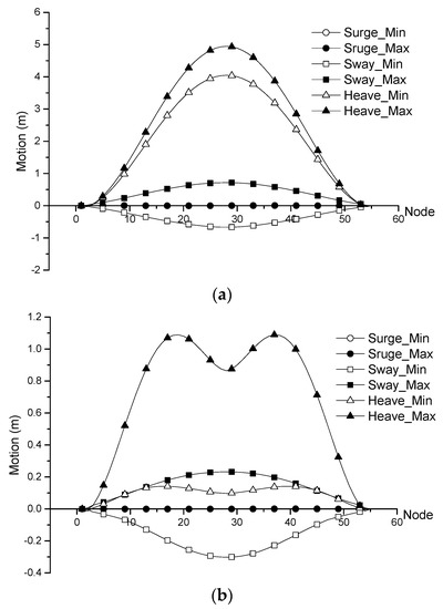
Figure 8.
Motion of SFT: (a) motion at each point of Type 1; (b) motion at each point of Type 2.
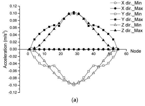
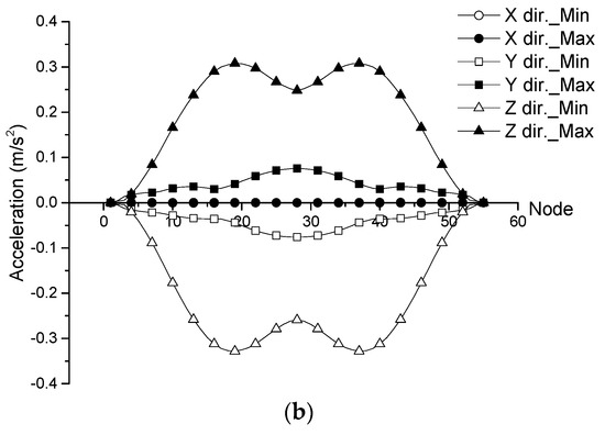
Figure 9.
Acceleration at each point of Type 1 and Type 2: (a) acceleration at each point of Type 1; (b) acceleration at each point of Type 2.
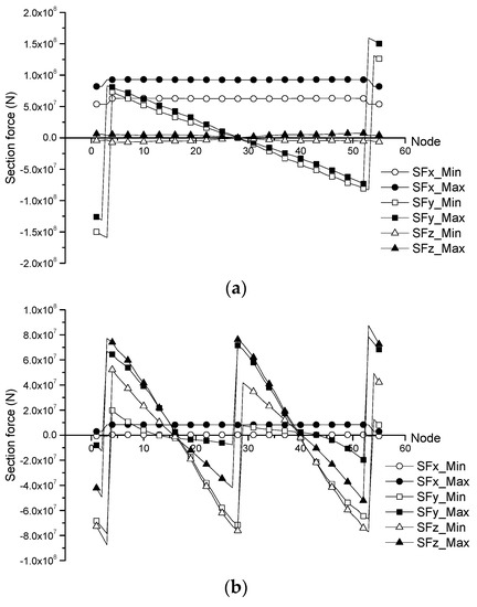
Figure 10.
Section force at each point of the SFT: (a) section force at each point of Type 1; (b) section force at each point of Type 2.
Figure 11.
Section moment at each point of the SFT: (a) section moment at each point of Type 1; (b) section moment at each point of Type 2.
For investigation of this model, the ABAQUS AQUA FE Program was used. When this FE program was applied to the new type structure, such as SFTs, verification of analysis model was very important. This analysis model was verified through comparison with hydraulic experimental study by Kim et al [16]. Oh et al [17] investigated hydraulic experimental study of SFT under a regular wave condition. The dimension of the SFT was 98 m of length and 23m of diameter. Through this experimental study, wave pressure, motion, and tension force of tether on SFT were evaluated. Kim et al [16] verified a comparison between hydraulic experimental study results and analyzed the results. Element SFTs and tethers for FE analysis were beam elements (b31) and truss elements (T3D2), respectively. Each tether and SFT were connected by multi-point constraint (MPC) option. Further, they proposed mesh size for FE analysis through parametric analysis. For boundary conditions, tethers were constrained by three directions and both ends of the SFT were only by way of constrained torsional rotation direction. As a result of sway motion of SFT, analysis results had very similar tendency with experimental results according to wave height and period. In addition, maximum and minimum tension force of tethers had similar results. Therefore, a verified analysis model of SFT was applied in this study.
First, Figure 8 shows the translation motion at each point of the SFT model. Here, the heave is for the linear vertical motion, the sway is for the linear transverse, and the surge is for the linear longitudinal motion. Moreover, they were expressed as a triangle, rectangle and circle, respectively. Additionally, the maximum value was plotted as a closed shape, and the open shape represents the minimum value in Figure 8. Figure 8a shows Type 1, and Figure 8b shows Type 2. It can be seen that the heave for Type 1 and Type 2 was the most responsive motion, because both have a BWR of 1.2. In Figure 8a, the maximum heave motion value was 5 m, and there was a fluctuation of approximately 1 m. Additionally, the sway motion value had a maximum of 0.5 m and minimum of 0.5 m and also fluctuated by approximately 0.5 m. Moreover, little surge motion occurred in the model, which was fixed with towers at both ends. On the other hand, in Figure 8b, showing Type 2, which is installed in the middle, as shown in Figure 6c, all motions were lower than those for Type 1. The maximum heave motion was 1.2 m due to the buoyancy of the model, and the sway motion, which acts in waves, was deformed by a maximum of 0.2 m and minimum of 0.3 m.
Next, Figure 9 illustrates the acceleration at each point of the SFT model. The acceleration caused by waves has a decisive effect when vehicles, trains, or life passes through the SFT. The smaller this value, the higher the serviceability. Figure 9a exhibits the acceleration in Type 1. It can be seen that the acceleration in the wave load acting direction (y-axis) and the buoyancy acting direction (z-axis) was almost similarly large, and the maximum value was 0.1 m/s2. Conversely, in Figure 9b, showing Type 2, the acceleration in the y-axis was smaller than the value in the z-axis. However, the value in the z-axis was 0.3 m/s2, which is larger than that in Type 1. Moreover, the value of the wave acting direction (y-axis) was decreased to 0.05 m/s2. This is because Type 2 has a middle anchorage, so that the deformation in the z-axis was controlled, as shown in Figure 8b.
Next, Figure 10 displays the section force of the wave load on the SFT model. Here, SFx means an axial force, and SFy and SFz indicate the shear forces on the y-axis and z-axis, respectively. Figure 10a shows the generated resistance force on Type 1. It can be found that there was almost no shear force in the z-direction (SFz), and it can be seen that the shear force in the y-direction (SFy) was the largest at the towers due to waves. The maximum axial force acting on the SFT was about 100 MN. Figure 10b shows the section force on Type 2. Since it was supported by a middle anchorage, the axial force (SFx) was decreased to approximately 10 MN, and the generated shear force (SFy, SFz) in the wave load direction (y) and the buoyancy direction (z) was almost the same, but the value was lower than that in Type 1. The shape of the shear force diagram for Type 2 also differs from that for Type 1.
Finally, Figure 11 plots the sectional moment on the SFT model. It can be seen that both Type 1 and Type 2 had a large torsional moment. Numerically, the torsional strength of Type 1 was greater than that of Type 2.
4. Parametric Study
4.1. Wave Height
As previously mentioned in Table 1, the wave condition was selected, with three variables, according to significant wave heights and periods of 3.5 m (5 s), 6.0 m (8 s) and 8.0 m (10 s). These conditions represented the time series, shown in Figure 7, applying the JONSWAP spectrum. The common variables of the analytical model include a BWR of 1.2, a main cable angle of 12 degrees, a tube external diameter of 23 m, and an installation depth of 70 m.
Figure 12 shows the motion, acceleration, reaction force, section force, and section moment in the SFT, according to wave heights. Figure 12a displays the motion of the suspended SFT, according to the wave height. As the wave height increased, the overall motion tended to grow. Moreover, it can be found that the motion in Type 2 was smaller than that in Type 1. In absolute terms, the heave motion was the largest due to the influence of the BWR, followed by the sway, which was deformation in the wave acting direction.
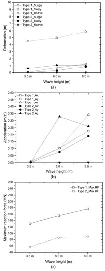
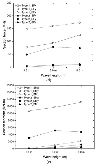
Figure 12.
Behavior of the SFT, according to the wave height: (a) motion of the SFT; (b) maximum acceleration on the SFT; (c) maximum reaction force on the foundation of the SFT; (d) maximum section force on the SFT; (e) maximum section moment in the SFT.
Figure 12b exhibits the maximum acceleration in the SFT, according to the wave height, without considering the position. It can be seen that the absolute maximum value tended in the upward direction as the wave height increased, but in the case of Type 2, the acceleration value significantly rose under the 6 m wave height condition. It can be judged that the acceleration was generated largely by the impact load of irregular waves, as shown in Figure 12a. It can be determined that the acceleration in Type 2 under the 8 m wave height condition was smaller than that under the 6 m condition, because in the case of the 6 m wave height, there was a smaller heave motion than in the case of the 8 m condition.
Figure 12c plots the maximum reaction force on the foundation of the SFT model, according to wave height, without considering the position. There was less reaction force on Type 2 than on Type 1, because it had one more anchorage to support. In terms of tendency, Type 1 was increased linearly, but in the case of Type 2, the slope was increased at the wave height of 6 m due to the influence of the heave.
When the wave force acted, cross-section forces, such as the shear force and the moment were generated in the SFT. As mentioned above, an axial force, SFx, was generated in the x-axis in the SFT, and a shear force, SFy and SFz, occurred in the wave load acting direction (y-axis) and the buoyancy direction (z-axis), respectively. These section forces at each point were plotted in Figure 10 and Figure 12d, representing the maximum section force on the foundation of the SFT, according to the wave height. Both Type 1 and Type 2 had the largest shear force, SFy, in the wave acting direction. In the case of Type 1, the section force on the SFT was decreased in the order of SFy, SFx and SFz. On the contrary, since Type 2 was supported by a middle anchorage, there was a lot of shear force, SFy, and not a lot of SFx and SFz.
Figure 12e plots the absolute maximum section moment at the foundation of the SFT, according to the wave height. It can be seen that the torsional moment (SFx) dominated in both Type 1 and Type 2. It can be considered that the torsion occurred in the arch shaped SFT model, because the wave acted in the y-axis, while heave motion was generated, as shown in Figure 8. For this reason, the torsional moment of Type 1, with the largest heave motion, was greater than that of Type 2.
4.2. Buoyancy–Weight Ratio (BWR)
In floating structures, BWR, the buoyancy-weight ratio, is a key factor. The buoyancy and weight can determine the initial tension of tethers, and the possibility of the rapid motion of structures implies that it depends on the BWR. In this section, the behavior of the proposed SFT was analyzed, considering the BWR. The common variables of the analytical model included a wave condition of 6 m (8 s), a main cable angle of 12 degrees, a tube external diameter of 23 m, and an installation depth of 70 m.
Figure 13 shows the motion, the acceleration, the reaction force, the section force, and the section moment in the SFT, according to BWR. Figure 13a displays the absolute maximum motion of the SFT, according to the BWR. It can be seen that the motion in Type 1 and Type 2 was significantly different. For Type 1, with open shapes, it was found that the heave motion grew as the BWR was increased. The deformation of the heave was increased by the buoyancy, as shown in Figure 13b. Maximum and minimum values at each point in the SFT were maintained at regular intervals. Figure 13c shows the heave motion in Type 2, according to the BWR. Comparing Figure 13b,c, the maximum heave value with a BWR of 1.3 was 6.3 m for Type 1. In contrast, the motion in Type 2 was decreased as the BWR was increased, as shown in Figure 13c. In addition, at a BWR of 1.1, it was found that the heave value was about 2 m, then above a BWR of 1.2, the motions were almost the same, at approximately 1.3 m. Moreover, at a BWR of 1.1, the SFT underwent a sudden slack and generated a negative heave motion of −1.7 m. This mainly occurred when the buoyancy is weak.
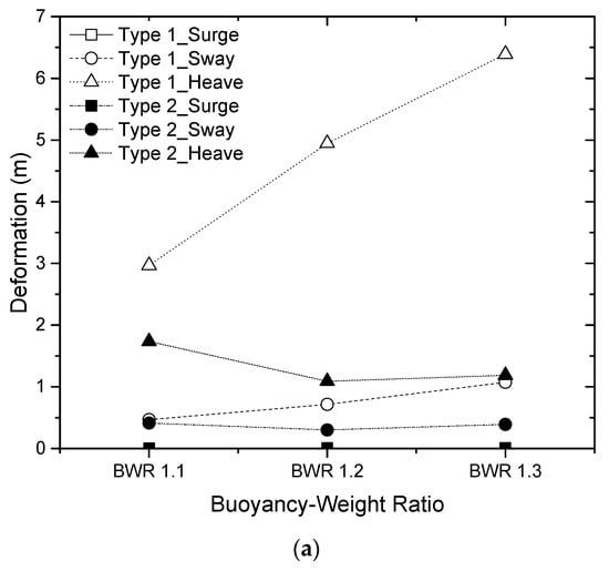
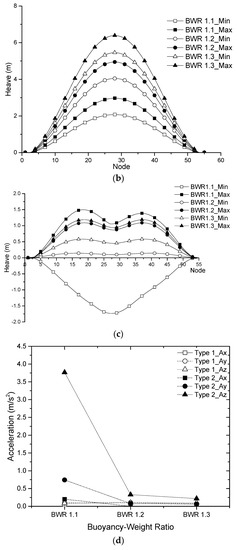
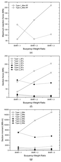
Figure 13.
Behavior of the SFT, according to the buoyancy-weight ratio: (a) maximum motion of the SFT; (b) heave motion of the SFT Type 1; (c) heave motion of the SFT Type 2; (d) maximum acceleration of the SFT; (e) maximum reaction force on the foundation of the SFT; (f) maximum section force of the SFT; (g) maximum section moment of the SFT.
Next, Figure 13d shows the absolute maximum acceleration of the SFT model, according to the BWR. Again, the open shape represents Type 1, and the closed shape represents Type 2. For Type 1, the acceleration value was less than 0.25 and was steady. For Type 2, however, it can be seen that the acceleration value in the z-axis direction, with a BWR of 1.1, had a large value, at 3.75 , and the value in the wave acting direction (y-axis) was 0.75 , which was much larger than that of Type 1. These figures are shown in Figure 13a–c. For Type 2, since the motion was stabilized with the rising initial tension, which was due to increasing the BWR, the acceleration was decreased.
Next, Figure 13e indicates the absolute maximum reaction force on the foundation of the SFT model, according to the BWR, and indicates the largest value of each point. In the case of Type 1, the reaction force was increased proportionally as the BWR was increased. In contrast to Type 2, the greatest motion occurred at a BWR of 1.1, declined at a BWR of 1.2, and was rebounded at a BWR of 1.3.
Next, Figure 13f,g plot the maximum section force and section moment of the SFT model, according to the BWR. For Type 1, the section force rose as the BWR was increased. Moreover, the shear force in the y-axis direction (SFy), which is the wave load acting direction, was the largest, followed by the axial force and, finally, the SFx. Here, the axial force is the sum of all tensile forces, as shown in Table 2.
Table 2.
Maximum and minimum axial section forces of Type 1 and Type 2.
Finally, Figure 13g illustrates the absolute maximum section moment of the SFT model, according to the BWR. The shear moment is also affected by motion. Type 1 and Type 2 were both under a great amount of torsion. It can be seen that this was proportional to the heave motion, and the section moment in the other directions was small (below 2000 MN-m).
4.3. Inclination Angle of the Main Cables
In this section, the behavior of the suspended SFT was analyzed, according to the inclination angle of the main cables. The inclination angles were set to 12 degrees, 25 degrees, and 35 degrees, as shown in Figure 14, to analyze the effect of the arrangement method of the main cable on the behavior of the SFT. The common variables of the analytical model include a wave condition of 6 m (8 s), a BWR of 1.2, a tube external diameter of 23 m, and an installation depth of 70 m.
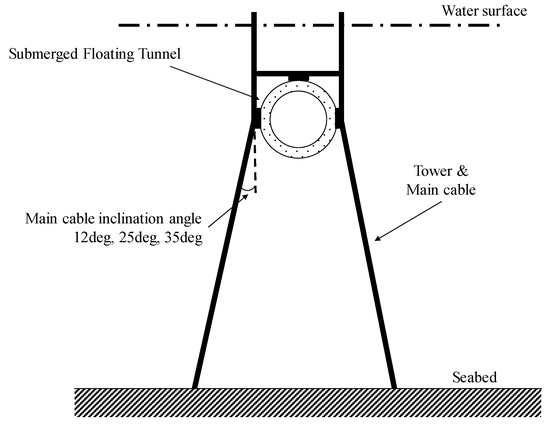
Figure 14.
Inclination angle of the main cables.
Figure 15 shows the motion, acceleration, reaction force, section force, and section moment of the SFT, according to the inclination angle of the main cable. Figure 15a displays the absolute maximum motion of the SFT, according to the inclination angle, which exhibits little change of motion with the variables. However, it can be seen that the sway motion of Type 2 increased when it was placed at 35 degrees. The sway value affects the change in the acceleration, which was approximately doubled, as shown in Figure 15b.
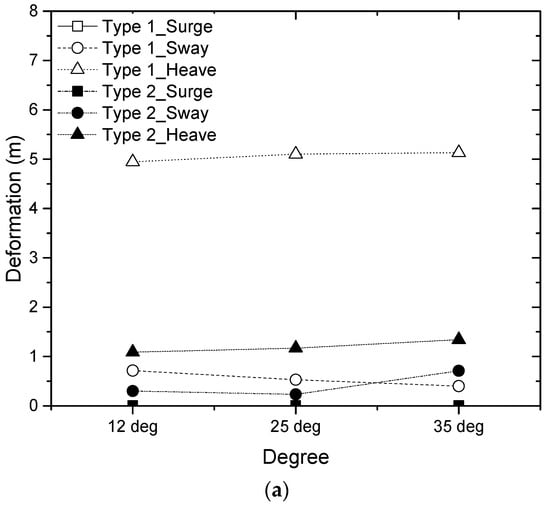
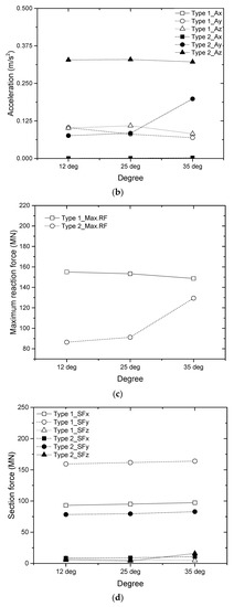
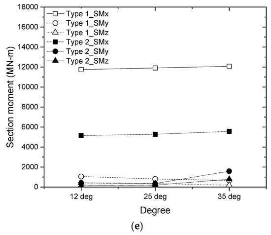
Figure 15.
Behavior of the SFT, according to the inclination angle of the main cable: (a) maximum motion of the SFT; (b) maximum acceleration of the SFT; (c) maximum reaction force on the foundation of the SFT; (d) maximum section force of the SFT; (e) maximum section moment of the SFT.
Next, Figure 15c indicates the absolute maximum reaction force on the foundation of the SFT model, according to the inclination of the main cable. In the case of Type 1, the reaction force decreased slightly as the angle increased. Conversely, for Type 2, the reaction force increased with the inclination angle. This is related to the lateral motion, and the reaction force increased with the rise of the sway motion, as shown in Figure 15a.
Next, Figure 15d,e display the maximum section force and section moment of the SFT model, according to the inclination angle. They were slightly elevated but showed almost similar values. It can be seen that 12 degrees, which is the smallest variable, can be sufficient to control the motion.
4.4. Diameter of the SFT
In this section, the diameter of the SFT was assumed to 17 m, 20 m and 23 m to analyze its effect on the behavior of the SFT. The common variables of the analytical model include a wave condition of 6 m (8 s), a BWR of 1.2, an inclination angle of the main cables of 12 degrees and an installation depth of 70 m.
With common analysis variables, the SFT model with the tube diameter has an almost similar motion as that shown in Figure 16a. The heave motion of Type 1 became smaller as the diameter increased. It can be seen that the BWR is set to 1.2, but it gained weight as the tube diameter increased. On the other hand, in the case of Type 2, it was seen that the motion was almost the same, the heave motion was 1.1 m, and the sway value was 0.4 m.
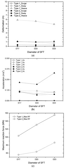
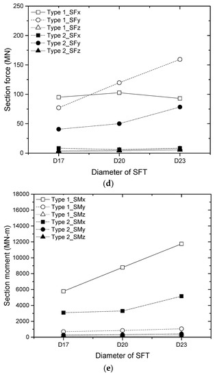
Figure 16.
Behavior of the SFT, according to the diameter of the SFT: (a) maximum motion of the SFT; (b) maximum acceleration of the SFT; (c) maximum reaction force on the foundation of the SFT; (d) maximum section force of the SFT; (e) maximum section moment of the SFT.
Figure 16b illustrates the absolute maximum acceleration of the SFT, according to the tube diameter. For Type 2, the greatest acceleration value was in the buoyancy acting direction (Az) in the case of the SFT with a 23 m diameter (D23). For Type 1, it can be seen that the acceleration was relatively small, compared to that of Type 2, because the fluctuation of the motion was relatively small.
Figure 16c shows the maximum reaction force at the foundation of the tether, and the maximum reaction force was increased by the diameter. This means that a large diameter causes the SFT to have a large weight. This creates a large inertial force and has a significant influence on the section force and moment. Figure 16d,e show the section force and section moment of the SFT under the external boundary conditions. These have a linear change tendency, compared with the motion of the SFT, according to the diameter of the SFT.
4.5. Installation Depth of the SFT
In this section, the installation depth of the SFT was set to 40 m, 70 m and 100 m from the sea level to analyze the effect on the behavior of the SFT. The common variables of the analytical model included a wave condition of 6 m (8 s), a BWR of 1.2, an inclination angle of the main cables of 12 degrees and a tube external diameter of 23 m.
Figure 17a illustrates the absolute maximum motion of the SFT, according to the installation depth (draft). The deeper the installation depth, the less the influence of waves, and the less the motion of the SFT. Compared with the sway motion, Type 1 and Type 2 had a similar behavior at a depth of 40 m, and the motion of Type 2 was reduced above a depth of 70 m, compared to that at 40 m. The cause of this can be determined by analyzing the heave motion of Type 2, as shown in Figure 17b. In Figure 17b, it can be seen that slack occurred at an installation depth of 40 m, and this phenomenon can greatly affect the acceleration, section force, reaction force, and so forth.
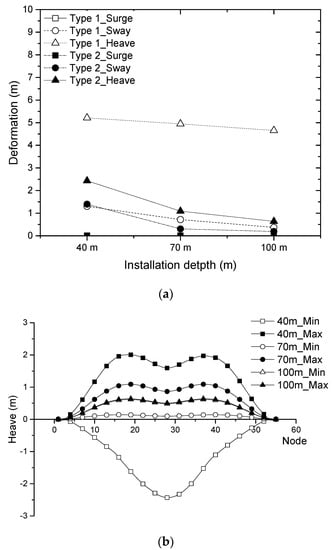
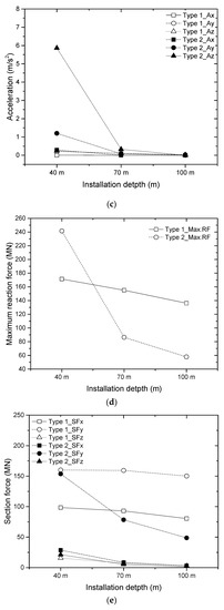
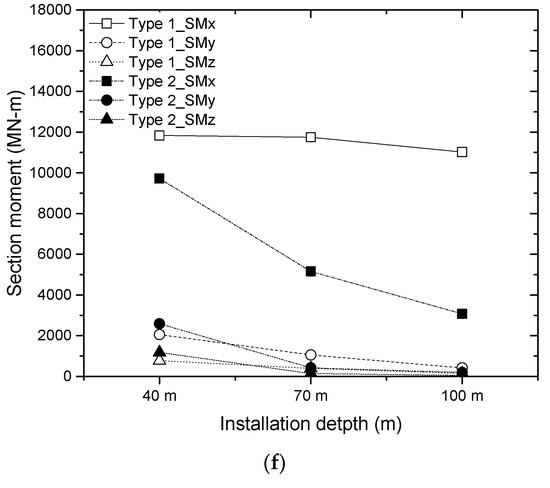
Figure 17.
Behavior of the SFT, according to the installation depth: (a) maximum motion of the SFT; (b) heave motion at each point of the SFT; (c) maximum acceleration of the SFT; (d) maximum reaction force on the foundation of the SFT; (e) maximum section force of the SFT; (f) maximum section moment of the SFT.
Figure 17c expresses the absolute maximum acceleration of the SFT model, according to the motion with drafts. It can be seen that the acceleration in the buoyancy acting direction (z-axis) at a depth of 40 m was 6 m/s2 due to the slack, but it decreased rapidly above a depth of 70 m. A directional acceleration of 70 m and an installation depth of 100 m were shown to have nearly similar values.
Figure 17d displays the absolute maximum reaction force on the foundation of the SFT, according to the draft. It can be seen that the reaction force of Type 2 at a depth of 40 m was 240 MN, which is larger than that of Type 1, with 170 MN. However, at a depth of 70 m, the force of Type 2 was much lower than that of Type 1. It can be seen that Type 2 was more affected by the installation depth.
Figure 17e,f exhibit the maximum section force and section moment of the SFT model, according to the draft. In the case of the maximum section force, the shear force in the wave acting direction (SFy) was the largest. Moreover, the deeper the installation depth, the less the axial force and the directional shear forces. It can be found that Type 2 was more susceptible to the depth due to slack, as shown in Figure 17b. In the case of the maximum section moment, it can be seen that the torsion was dominant, as in the case of other variables. Since the section moment of Type 2, where slack occurred, rapidly decreased, it can be seen that it is necessary to prevent the slack.
5. Summary and Conclusions
In this study, two types of suspended SFTs were proposed to analyze their hydrodynamic behavior. The main variables were the wave conditions, cross-sectional diameters, buoyancy weight ratios, inclination angles of the main cables, and installation depth of the SFT.
- Wave condition: as the significant wave height increased, the motion of both Type 1 and Type 2 was increased.
- BWR: The behavior of Type 1 and Type 2 differed, depending on the BWR. For Type 2, the acceleration, reaction force, and section force were all increased, as negative motion occurred due to the slack in the BWR 1.1. On the other hand, for Type 1, as the BWR increased, the heave motion increased, and the acceleration, reaction force, and section force increased proportionally.
- Inclination angle of the main cables: it can be seen that the behavior of Type 1 and Type 2 differed, as the inclination angle of the main cables increased. In the case of Type 2, the acceleration, section force, reaction force, etc. increased as the motion in the wave acting direction increased. In contrast, the behavior of Type 1 decreased as the angle increased.
- Diameter of the tube: The acceleration, section force, and reaction force increased as the diameter of the tube grew under the aforementioned conditions. It can be seen that the SFT with the tube of a large dimeter is disadvantageous economically and mechanically.
- Installation depth of the SFT: as the installation depth of the SFT increased, the wave breaking impact generally decreased, and the motion decreased. However, in the case of a depth of 40 m, Type 2 experienced slack, and the acceleration, section force and reaction force were greatly increased, which is a condition that should be avoided.
- Comprehensive remarks: overall, it can be seen that the Type 2 SFT was superior from a hydrodynamic point of view. However, a detailed hydrodynamic analysis must be performed to avoid the conditions that previously produced slack. In addition, in the case of acceleration being generated by motion, the design should be reviewed to ensure safe conditions, according to the traffic passage.
Author Contributions
conceptualization, W.-S.P. and Y.Y.; software, S.K.; formal analysis, D.W.; investigation, D.W. and S.K.; resources, D.W.; data curation, J.S.; writing—original draft preparation, D.W and J.S; writing—review and editing, D.W. and J.S.; visualization, D.W.; supervision, W.-S.P; project administration, W.-S.P.; funding acquisition, W.-S.P.
Funding
This work was supported by the National Research Foundation of Korea (NRF), the grant for which was funded by the Korea government (MSIT) (No. 2017R1A5A1014883).
Conflicts of Interest
The authors declare that they have no conflicts of interest.
Abbreviations
| the cross-sectional area | |
| the added mass coefficient (with a cross-sectional area as a reference area) | |
| the drag coefficient | |
| the diameter | |
| the sectional drag force | |
| a loft force | |
| normal force | |
| a tangential force | |
| a torsion moment | |
| the fluid particle (waves and/or current) velocity | |
| the fluid particle acceleration | |
| the mass density of the fluid | |
| the wavelength |
References
- Zanchi, F. Archimedes Bridge; Floornature: Naple, Italy, 2002. [Google Scholar]
- Martire, G. The Development of Submerged Floating Tunnels as an Innovative Solution for Waterway Crossings. Ph.D. Thesis, Construction Engineering, University of Naples “Federico II”, Naples, Italy, 2010. [Google Scholar]
- Mazzolani, F.M.; Landolfo, R.; Faggiano, B.; Esposto, M.; Martire, G.; Perotti, F.; Di Pilato, M.; Barbella, G.; Fiorentino, A. The Archimede’s Bridge Prototype in Qiandao Lake (PR of China)—Design Report; Research Project Report; Sino-Italian Joint Laboratory of Archimedes Bridge (SIJLAB): Qiandao, China, 2007. [Google Scholar]
- NPRA (Norwegian Public Roads Administration). A Feasibility Study—How to Cross the Wide and Deep Sognefjord; Norwegian Public Roads Administration: Western Region, Oslo, Norway, 2011. [Google Scholar]
- Lin, H.; Xiang, Y.Q.; Yang, Y.S. Vehicle-tunnel coupled vibration analysis of submerged floating tunnel due to tether parametric excitation. Mar. Struct. 2019, 67. [Google Scholar] [CrossRef]
- Xiang, Y.Q.; Yang, Y. Spatial dynamic response of submerged floating tunnel under impact load. Mar. Struct. 2017, 53, 20–31. [Google Scholar] [CrossRef]
- Seo, S.I.; Mun, H.S.; Lee, J.H.; Kim, J.H. Simplified analysis for estimation of the behavior of a submerged floating tunnel in waves and experimental verification. Mar. Struct. 2015, 44, 142–158. [Google Scholar] [CrossRef]
- Xiang, Y.Q.; Chen, Z.Y.; Yang, Y.; Lin, H.; Zhu, S. Dynamic response analysis for submerged floating tunnel with anchor-cables subjected to sudden cable breakage. Mar. Struct. 2018, 59, 179–191. [Google Scholar] [CrossRef]
- Lu, W.; Ge, F.; Wang, L.; Wu, X.D.; Hong, Y.S. On the slack phenomena and snap force in tethers of submerged floating tunnels under wave conditions. Mar. Struct. 2011, 23, 358–376. [Google Scholar] [CrossRef]
- Jin, C.; Kim, M.H. Time-Domain Hydro-Elastic Analysis of a SFT (Submerged Floating Tunnel) with Mooring Lines under Extreme Wave and Seismic Excitations. Appl. Sci. 2018, 8, 2386. [Google Scholar] [CrossRef]
- Chen, Z.Y.; Xiang, Y.Q.; Lin, H.; Yang, Y. Coupled Vibration Analysis of Submerged Floating Tunnel System in Wave and Current. Appl. Sci. 2018, 8, 1311. [Google Scholar] [CrossRef]
- Won, D.; Kim, S. Feasibility Study of Submerged Floating Tunnels Moored by an Inclined Tendon System. Int. J. Steel Struct. 2018, 18, 1191–1199. [Google Scholar] [CrossRef]
- Veritas, D.N. DNV-RP-C205 Environmental Conditions and Environmental Loads; Det Norske Veritas: Oslo, Norway, 2010. [Google Scholar]
- Simulia Inc. ABAQUS 6.14 User’s Manual; Dassault Systems: Providence, RI, USA, 2014. [Google Scholar]
- Hasselmann, K.; Barnett, T.P.; Bouws, E.; Carlson, H.; Cartwright, D.E.; Enke, K.; Ewing, J.A.; Gienapp, H.; Hasselmann, D.E.; Kruseman, P.; et al. Measurements of wind-wave growth and swell decay during the Joint North Sea Wave Project (JONSWAP); Ergnzungsheft zur Deutschen Hydrographischen Zeitschrift Reihe: Delft, The Netherland, 1973. [Google Scholar]
- Kim, S.; Park, W.S.; Won, D. Hydrodynamic Analysis of Submerged Floating Tunnel Structures by Finite Element Analysis. J. Korean Soc. Civ. Eng. 2016, 36, 955–967. [Google Scholar] [CrossRef]
- Oh, S.H.; Park, W.S.; Jang, S.C.; Kim, D.H. Investigation on the behavioral and hydrodynamic characteristics of submerged floating tunnel based on regular wave experiments. J. Korean Soc. Civ. Eng. 2013, 33, 1887–1895. [Google Scholar] [CrossRef]
© 2019 by the authors. Licensee MDPI, Basel, Switzerland. This article is an open access article distributed under the terms and conditions of the Creative Commons Attribution (CC BY) license (http://creativecommons.org/licenses/by/4.0/).