Analysis of the Effect of Vortex Generator Spacing on Boundary Layer Flow Separation Control


Abstract
1. Introduction
2. Methods
2.1. Numerical Conditions
2.1.1. Large Eddy Simulation
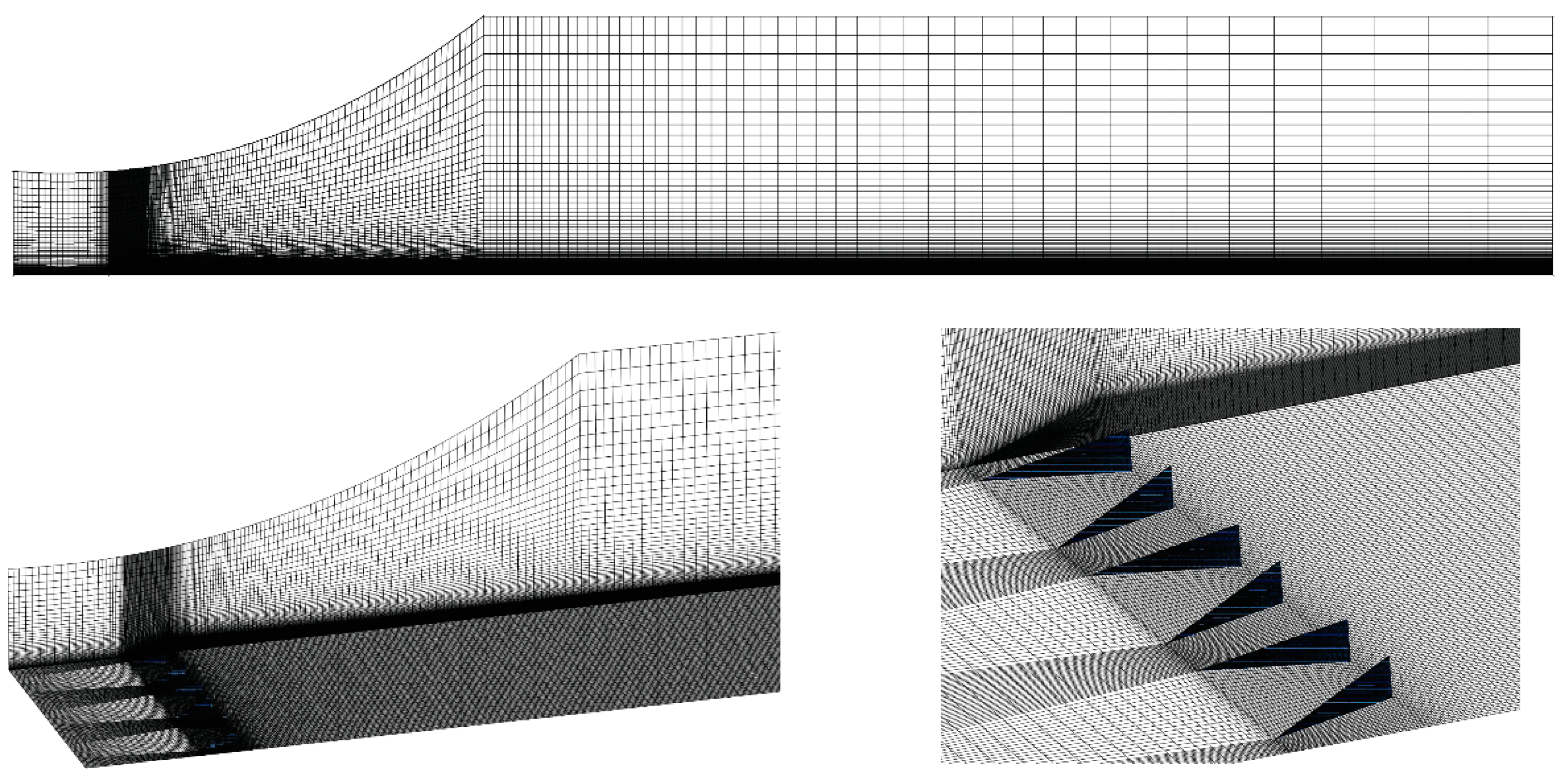
2.1.2. Mesh Development
2.1.3. Computational Setup
2.2. Experimental Setup
3. Results and Discussion
3.1. Analysis of the CFD Calculation Results
3.2. Analysis of the Experimental Results
4. Conclusions
Author Contributions
Funding
Conflicts of Interest
Nomenclature
| Δt | Unsteady computational physical time step (s) |
| β | Angle between vortex generators and incoming flow (°) |
| l | Vortex generators chord length (mm) |
| H | Vortex generators height (mm) |
| S | Distance between the trailing edge of the vortex generators in the opposite direction |
| λ | Distance between the trailing edge of the vortex generators in the same direction |
| CΔp | Pressure loss coefficient at the inlet and outlet of the calculation domain |
| Pinlet | Total pressure at the inlet |
| Poutlet | Total pressure at the outlet |
| RE | The value obtained using the Richardson extrapolation |
| R | The ratio of errors |
| p | The order of accuracy |
| Cp | Airfoil surface static pressure coefficient |
| Cl | Lift coefficient of airfoil |
| Cd | Drag coefficient of airfoil |
| Ulocal | Local velocity |
| U | Inlet velocity |
| Q | Vortex core criterion |
| Ω | Vortex core vorticity |
| r | Vortex core radius |
| Δz | The distance between the two vortex cores |
| <u> | Time-averaged velocity |
| Clean | Airfoil without VGs |
Abbreviations
| VGs | Vortex generators |
| LES | Large eddy simulation |
| AoA | Angle-of-attack |
| CFD | Computational fluid dynamics |
| NCEPU | North China Electric Power University |
| NPU | Northwest Polytechnic University |
| Delft | Delft University |
| APG | Adverse pressure gradient |
| ZPG | Zero pressure gradient |
References
- Wang, X.; Ye, Z.; Kang, S.; Hu, H. Investigations on the Unsteady Aerodynamic Characteristics of a Horizontal-Axis Wind Turbine during Dynamic Yaw Processes. Energies 2019, 12, 3124. [Google Scholar] [CrossRef]
- Li, X.; Yang, K.; Wang, X. Experimental and Numerical Analysis of the Effect of Vortex Generator Height on Vortex Characteristics and Airfoil Aerodynamic Performance. Energies 2019, 12, 959. [Google Scholar] [CrossRef]
- Ma, L.; Wang, X.; Zhu, J.; Kang, S. Dynamic Stall of a Vertical-Axis Wind Turbine and Its Control Using Plasma Actuation. Energies 2019, 12, 3738. [Google Scholar] [CrossRef]
- Macquart, T.; Maheri, A.; Busawon, K. Microtab dynamic modelling for wind turbine blade load rejection. Renew. Energy 2014, 64, 144–152. [Google Scholar]
- Ebrahimi, A.; Movahhedi, M. Wind turbine power improvement utilizing passive flow control with microtab. Energy 2018, 150, 575–582. [Google Scholar] [CrossRef]
- Kametani, Y.; Fukagata, K.; Orlu, R.; Schlatter, P. Effect of uniform blowing/suction in a turbulent boundary layer at moderate Reynolds number. Int. J. Heat Fluid Flow 2015, 55, 132–142. [Google Scholar] [CrossRef]
- Ziadé, P.; Feero, M.A.; Sullivan, P.E. A numerical study on the influence of cavity shape on synthetic jet performance. Int. J. Heat Fluid Flow 2018, 74, 187–197. [Google Scholar] [CrossRef]
- Yang, H.; Jiang, L.-Y.; Hu, K.-X.; Peng, J. Numerical study of the surfactant-covered falling film flowing down a flexible wall. Eur. J. Mech. Fluids 2018, 72, 422–431. [Google Scholar] [CrossRef]
- Barlas, T.K.; van Kuik, G.A.M. Review of state of the art in smart rotor control research for wind turbines. Prog. Aerosp. Sci. 2010, 46, 1–27. [Google Scholar] [CrossRef]
- Johnson, S.J.; Baker, J.P.; Dam, C.P.V. An overview of active load control techniques for wind turbines with an emphasis on microtabs. Wind Energy 2010, 13, 239–253. [Google Scholar] [CrossRef]
- Lin, J.C. Review of research on low-profile vortex generators to control boundary-layer separation. Prog. Aerosp. Sci. 2002, 38, 389–420. [Google Scholar] [CrossRef]
- Wang, H.; Zhang, B.; Qiu, Q.; Xu, X. Flow control on the NREL S809 wind turbine airfoil using vortex generators. Energy 2017, 118, 1210–1221. [Google Scholar] [CrossRef]
- Taylor, H.D. The Elimination of Diffuser Separation by Vortex Generators; Report No. R-4012-3; United Aircraft Corporation: Moscow, Russia, June 1947. [Google Scholar]
- Khoshvaght-Aliabadi, M.; Sartipzadeh, O.; Alizadeh, A. An experimental study on vortex-generator insert with different arrangements of delta-winglets. Energy 2015, 82, 629–639. [Google Scholar] [CrossRef]
- Skullong, S.; Promvonge, P.; Thianpong, C.; Pimsarn, M. Thermal performance in solar air heater channel with combined wavy-groove and perforated-delta wing vortex generators. Appl. Therm. Eng. 2016, 100, 611–620. [Google Scholar] [CrossRef]
- Rao, D.; Kariya, T. Boundary-layer submerged vortex generators for separation control—An exploratory study. In Proceedings of the 1st National Fluid Dynamics Conference, Cincinnati, OH, USA, 25–28 July 1998; American Institute of Aeronautics and Astronautics: Washington, DC, USA, 1988; pp. 839–846. [Google Scholar]
- Lin, J.C.; Robinson, S.K.; McGhee, R.J.; Valarezo, W.O. Separation control on high-lift airfoils via micro-vortex generators. J. Aircr. 1994, 31, 1317–1323. [Google Scholar] [CrossRef]
- Bragg, M.B.; Gregorek, G.M. Experimental study of airfoil performance with vortex generators. J. Aircr. 1987, 24, 305–309. [Google Scholar] [CrossRef]
- Yanagihara, J.I.; Torii, K. Enhancement of laminar boundary layer heat transfer by a vortex generator. JSME Int. J. 1992, 35, 400–405. [Google Scholar] [CrossRef]
- Fiebig, M.; Valencia, A.; Mitra, N.K. Local heat transfer and flow losses in fin-and-tube heat exchangers with vortex generators: A comparison of round and flat tubes. Exp. Therm. Fluid Sci. 1994, 8, 35–45. [Google Scholar] [CrossRef]
- Reuss, R.L.; Hoffman, M.J.; Gregorek, G.M. Effects of surface roughness and vortex generators on the NACA 4415 airfoil. Vortex Augment. Turbines 1995, 12, 442–472. [Google Scholar]
- Godard, G.; Stanislas, M. Control of a decelerating boundary layer. Part 1: Optimization of passive vortex generators. Aerosp. Technol. 2006, 10, 181–191. [Google Scholar] [CrossRef]
- Godard, G.; Stanislas, M. Control of a decelerating boundary layer. Part 2: Optimization of slotted jets vortex generators. Aerosp. Sci. Technol. 2006, 10, 394–400. [Google Scholar] [CrossRef]
- Godard, G.; Stanislas, M. Control of a decelerating boundary layer. Part 3: Optimization of round jets vortex generators. Aerosp. Sci. Technol. 2006, 10, 455–464. [Google Scholar] [CrossRef]
- Yang, K.; Zhang, L.; Xu, J.Z. Simulation of aerodynamic performance affected by vortex generators on blunt trailing-edge airfoils. Sci. China Ser. E Technol. Sci. 2010, 53, 1–7. [Google Scholar] [CrossRef]
- Zhen, T.K.; Zubair, M.; Ahmad, K.A. Experimental and Numerical Investigation of the Effects of Passive Vortex Generators on Aludra UAV Performance. Chin. J. Aeronaut. 2011, 24, 577–583. [Google Scholar] [CrossRef]
- Lishu, H.; Zhide, Q. Experimental Research on Control Flow over Airfoil Based on Vortex Generator and Gurney Flap. Acta Aeronaut. Astronaut. Sin. 2011, 32, 1429–1434. [Google Scholar]
- Delnero, J.S.; Leo, J.M.D.; Camocardi, M.E. Experimental study of vortex generators effects on low Reynolds number airfoils in turbulent flow. Int. J. Aerodyn. 2012, 2, 50–72. [Google Scholar] [CrossRef]
- Velte, C.M.; Hansen, M.O.L. Investigation of flow behind vortex generators by stereo particle image velocimetry on a thick airfoil near stall. Wind Energy 2013, 16, 775–785. [Google Scholar] [CrossRef]
- Sørensen, N.N.; Zahle, F.; Bak, C. Prediction of the Effect of Vortex Generators on Airfoil Performance. J. Phys. Conf. Ser. 2014, 524, 012019. [Google Scholar] [CrossRef]
- Manolesos, M.; Voutsinas, S.G. Experimental investigation of the flow past passive vortex generators on an airfoil experiencing three-dimensional separation. J. Wind Eng. Ind. Aerodyn. 2015, 142, 130–148. [Google Scholar] [CrossRef]
- Gao, L.; Zhang, H.; Liu, Y.; Han, S. Effects of vortex generators on a blunt trailing-edge airfoil for wind turbines. Renew. Energy 2015, 76, 303–311. [Google Scholar] [CrossRef]
- Fouatih, O.M.; Medale, M.; Imine, O.; Imine, B. Design optimization of the aerodynamic passive flow control on NACA 4415 airfoil using vortex generators. Eur. J. Mech. B/Fluids 2016, 56, 82–96. [Google Scholar] [CrossRef]
- Zhang, L.; Li, X.; Yang, K.; Xue, D. Effects of vortex generators on aerodynamic performance of thick wind turbine airfoils. J. Wind Eng. Ind. Aerodyn. 2016, 156, 84–92. [Google Scholar] [CrossRef]
- Martínez-Filgueira, P.; Fernandez-Gamiz, U.; Zulueta, E.; Errasti, I.; Fernandez-Gauna, B. Parametric study of low-profile vortex generators. Int. J. Hydrog. Energy 2017, 42, 17700–17712. [Google Scholar] [CrossRef]
- Brüderlin, M.; Zimmer, M.; Hosters, N.; Behr, M. Numerical simulation of vortex generators on a winglet control surface. Aerosp. Sci. Technol. 2017, 71, 651–660. [Google Scholar] [CrossRef]
- Gageik, M.; Nies, J.; Klioutchnikov, I.; Olivier, H. Pressure wave damping in transonic airfoil flow by means of micro vortex generators. Aerosp. Sci. Technol. 2018, 81, 65–77. [Google Scholar] [CrossRef]
- Baldacchino, D.; Simao Ferreira, C.; De Tavernier, D.A.M. Experimental parameter study for passive vortex generators on a 30% thick airfoil. Wind Energy 2018, 21, 118–132. [Google Scholar] [CrossRef]
- Kundu, P.; Sarkar, A.; Nagarajan, V. Improvement of performance of S1210 hydrofoil with vortex generators and modified trailing edge. Renew. Energy 2019, 142, 643–657. [Google Scholar] [CrossRef]
- Mereu, R.; Passoni, S.; Inzoli, F. Scale-resolving CFD modeling of a thick wind turbine airfoil with application of vortex generators: Validation and sensitivity analyses. Energy 2019, 187, 115969. [Google Scholar] [CrossRef]
- Manolesos, M.; Papadakis, G.; Voutsinas, S.G. Revisiting the assumptions and implementation details of the BAY model for vortex generator flows. Renew. Energy 2020, 146, 1249–1261. [Google Scholar] [CrossRef]
- Li, X.; Yang, K.; Hu, H.; Wang, X.; Kang, S. Effect of Tailing-Edge Thickness on Aerodynamic Noise for Wind Turbine Airfoil. Energies 2019, 12, 270. [Google Scholar] [CrossRef]
- Smagorinsky, J. General Circulation Experiments with the Primitive Equations, Part 1, Basic Experiments. Mon. Weather Rev. 1963, 91, 99–164. [Google Scholar] [CrossRef]


| Setting Angle β (°) | Length l (mm) | Height H (mm) | S/H | λ/H |
|---|---|---|---|---|
| 20 | 17 | 6 | 7 | 3, 5, 7, 9 |
| Variables | Mesh | Richardson Extrapolation | ||||
|---|---|---|---|---|---|---|
| Coarse | Medium | Fine | RE | p | R | |
| 0.3635 | 0.3628 | 0.3622 | 0.3620 | 2.75 | 0.22 | |
| Installation Angle β (°) | Length l (mm) | Height H (mm) | Spacing S/H | Pitch Distance λ/H |
|---|---|---|---|---|
| 20 | 17 | 5 | 5 | 3, 5, 7, 9 |
| Case | Stall Angle-of-Attack | Increase of Maximum Cl | Decrease of Cd at 18° | Increase of Lift–Drag Ratio at 18° |
|---|---|---|---|---|
| Clean | 8° | 0% | 0% | 0% |
| λ/H = 3 | 18° | 45.67% | 82.06% | 741.03% |
| λ/H = 5 | 18° | 48.77% | 83.28% | 821.86% |
| λ/H = 7 | 18° | 48.32% | 78.43% | 612.06% |
| λ/H = 9 | 16° | 30.20% | 13.06% | 55.06% |
© 2019 by the authors. Licensee MDPI, Basel, Switzerland. This article is an open access article distributed under the terms and conditions of the Creative Commons Attribution (CC BY) license (http://creativecommons.org/licenses/by/4.0/).
Share and Cite
Li, X.-k.; Liu, W.; Zhang, T.-j.; Wang, P.-m.; Wang, X.-d. Analysis of the Effect of Vortex Generator Spacing on Boundary Layer Flow Separation Control. Appl. Sci. 2019, 9, 5495. https://doi.org/10.3390/app9245495
Li X-k, Liu W, Zhang T-j, Wang P-m, Wang X-d. Analysis of the Effect of Vortex Generator Spacing on Boundary Layer Flow Separation Control. Applied Sciences. 2019; 9(24):5495. https://doi.org/10.3390/app9245495
Chicago/Turabian StyleLi, Xin-kai, Wei Liu, Ting-jun Zhang, Pei-ming Wang, and Xiao-dong Wang. 2019. "Analysis of the Effect of Vortex Generator Spacing on Boundary Layer Flow Separation Control" Applied Sciences 9, no. 24: 5495. https://doi.org/10.3390/app9245495
APA StyleLi, X.-k., Liu, W., Zhang, T.-j., Wang, P.-m., & Wang, X.-d. (2019). Analysis of the Effect of Vortex Generator Spacing on Boundary Layer Flow Separation Control. Applied Sciences, 9(24), 5495. https://doi.org/10.3390/app9245495