System Reliability Assessment with Imprecise Probabilities

Abstract

The exact statistical characteristics of some components may be unavailable because of the limited sample information in practical engineering. One challenge that system reliability analysis faces is dealing with limited sample sizes, which introduces the potential for a high level of uncertainty in the analysis results. In this paper, we propose a procedure for the reliability analysis of complex systems with a limited number of samples. Bayesian inference is used to estimate the parameter intervals of the life distributions of the components with a limited number of samples. Then, probability boxes (p-box) are constructed from the parameter intervals to represent the life distributions of the components with a limited number of samples. In addition, the theory of survival signature is applied to calculate the reliability of the system with a mixture of precise and imprecise knowledge of the life distributions of the components. Finally, two numerical examples are given to illustrate the validity of the methods.

1. Introduction

In recent years, the rapid development of science and technology has made today′s engineering systems (e.g., the control system of the unmanned helicopter) more powerful and complex. However, the resulting reliability problems have become increasingly prominent and the losses caused by failures are huge or even catastrophic. Therefore, it becomes even more important to perform system reliability analysis in order to mitigate the risks and to ensure system safety [1,2,3,4].

Traditionally, reliability analysis is based on large numbers of samples, which are used to perform statistical inferences. However, in many high-tech fields, such as aerospace, only a limited number of failure data samples are available due to the increased component or system reliability, cost constraints, or other reasons. Limited samples lead to the presence of epistemic uncertainty over the distributional parameters, which make the traditional research method based on a large number of samples no longer applicable [5,6,7]. Hence, it is of great significance to develop an effective and efficient reliability analysis method for complex systems under limited samples [8,9].

In general, the reliability analysis methods for limited samples can be roughly divided into two categories. One is the method based on virtual sample generation, which transform limited sample problems into large sample problems for processing, such as bootstrap [10,11] and support vector machine methods [12,13]. The second comprises methods based on Bayesian theory, which combine multiple forms of information for statistical inference. Dai et al. [14] proposed a Bayesian Monte Carlo method for high-reliability relay protectors obeying the Weibull distribution, for which limited failure data were available. Tripathi et al. [15] investigated the estimation procedure for the parameter, reliability, and hazard functions of the inverted exponential distribution under progressive type-II censored data in the Bayesian framework. Fabrizi et al. [16] proposed a generalized inverse Gaussian prior to lognormal linear regression models and discussed model parameter selection under small and medium sample sizes. For the problem that it is difficult to calculate the posterior distribution of complex distribution models, Soliman et al. [17] investigated the problem of point and interval estimations for the modified Weibull distribution using a type-II progressively censored sample based on the Markov Chain Monte Carlo (MCMC) approach. Singh et al. [18] derived Bayesian estimations of the hybrid censored lognormal distribution. In addition, Hamada et al. [19] wrote a book on the use of Bayesian theory in reliability assessment.

As is clear from the literature, the major focus of recent research has been on the processing of limited samples to get a reasonable result during reliability analysis of a complex system. In this paper, an efficient and effective method for reliability analysis of complex systems is proposed based on the theories p-box and survival signature. The rest of the paper is organized as follows: Section 2 gives a brief description of the theory of Bayesian interval estimation and p-box. As examples, the p-boxes of the exponential and Weibull distributions are obtained analytically, based on the Bayesian theory. In Section 3, we present a method for the reliability analysis of complex systems with limited samples, based on the theories of p-box and survival signature, while Section 4 gives two numerical examples to illustrate the application of the proposed approach. Finally, Section 5 presents the conclusions of the paper and some ideas for related future work.

2. A p-box Method Based on Bayesian Theory

Aleatory and epistemic uncertainties included in limited samples have an important impact on system reliability analysis. Recently, many methods were proposed to deal with epistemic uncertainty, such as fuzzy sets, information difference theory, interval analysis, evidence theory, etc. [20,21,22]. All these methods have their own desirable and undesirable features—such as the approach of evidence theory, especially the appropriateness of Dempster’s rule for combining evidence, which is somewhat controversial [23]. In this section, the theory of probability box (p-box) is used to construct the parameter intervals to represent the life distributions of the components with a limited number of samples.

The theory of p-box is used to analyze both aleatory and epistemic uncertainty by combining the probability theory and interval arithmetic. It is an effective method that uses the lower and upper limit of the CDF (or life distribution) to represent the real distribution function. Ferson et al. [24] first proposed the concept of p-box, introduced the related theory, and proposed some calculation methods. Based on the work by Ferson, many theoretical properties and practical aspects of p-box have already been studied [25,26,27]. In this paper, we present a p-box method based on Bayesian interval estimation.

Bayesian theory combines the prior, population, and sample information for statistical inference, which can give more accurate estimation results in the case of limited samples. The advantage of interval estimation is that it uses intervals to represent distribution parameters, avoiding the error between point estimates and true values. The core of Bayesian theory is the Bayesian Equation [19]:

$$p(\theta |t)=\frac{f(t|\theta )p(\theta )}{{\displaystyle {\int }_{U}f(t|\theta )p(\theta )\mathrm{d}\theta }}$$

(1)

where θ is the parameter of the population distribution from which the sample is drawn and U represents the parameter space; p(θ) and p(θ|t) are the prior and posterior distribution of θ respectively; f(t|θ) stands for the likelihood function of the sample, while the vector x = (x₁,…,x_n) is a random sample from the population.

Suppose that there is a sample t = (x₁, …, x_n) subject to the distribution of f(t|θ), and the posterior distribution of θ is p(θ|x). For a given probability, 1 − α (0 < α < 1), where α is the significance level, if we can find two statistics from the posterior distribution such that P(θ_l < θ < θ_u) = 1 − α, then the Bayesian confidence interval of parameter θ at the confidence level 1 − α can be written as [θ_l, θ_u]. In this paper, the significance level is α = 0.05, or conversely, the confidence level is 95%. Therefore, the 0.025 and 0.975 quantiles in the posterior distribution can be used as the lower and upper limits of parameter θ, respectively.

When the prior and likelihood are of a specific form (e.g., exponential, gamma, and normal distribution), the posterior distribution follows the same form as the prior, and the prior and likelihood are said to conjugate. In these cases, the inferences based on the posterior distributions are straightforward and simpler. Conjugate priors for the indicated parameters of commonly used likelihood distributions are listed in

Table 1. Conjugate distributions.

Likelihood Distribution	Conjugate Prior
Normal	Normal, inverse gamma
Exponential	Gamma
Uniform	Pareto
Lognormal	Normal, gamma
Poisson	Gamma
Binomial	Beta
Pareto	Gamma
Negative binomial	Beta
Geometric	Beta
Gamma	Gamma

. For more detail, please refer to Reference [28].

In this section, the exponential distribution, which is one of the most commonly used lifetime distributions in reliability engineering, is used to illustrate the method for solving Bayesian models by using conjugate priors. The probability density function of exponential distribution is:

$$f(t)=\lambda e^{-\lambda t},t>0$$

(2)

where λ is the failure rate. Suppose there are n component failure times t = (t₁, …, t_n) that follow the exponential distribution. In this paper, we assume that the form of prior information is a prior failure data sample T = (T₁, …, T_N), which also follows the exponential distribution. Therefore, according to the Bayesian theory and the properties of the conjugate prior distribution, the posterior distribution of λ is [19]:

$$p(\lambda |t)~\mathrm{gamma}(\mu +n,\nu +{\displaystyle \sum _{i=1}^n{t}_i})$$

(3)

where μ = N and $\nu ={\displaystyle {\sum }_{i=1}^N{T}_i}$ are the numbers of elements in the prior failure data and total failure time, respectively. By calculating the 0.025 and 0.975 quantiles of p(λ| t), respectively, we can obtain the 95% Bayesian confidence interval of parameter λ as [λ_l, λ_u].

For some distributions, although they do not have conjugate priors, they can be transformed to distribution functions that have conjugate priors. For example, the probability density function of the two-parameter Weibull distribution is:

$$f\left(t,\alpha ,\beta \right)=\frac{\beta }{\alpha }{\left(\frac{t}{\alpha }\right)}^{\beta -1}\exp \left[-{\left(\frac{t}{\alpha }\right)}^{\beta }\right],t\ge 0$$

(4)

where α and β are the scale and shape parameters, respectively. There is no conjugate prior for the Weibull distribution. Under the assumption that β is known, the Weibull distribution can be transformed into the exponential distribution and then the posterior distribution of α can be obtained [29,30]. Assuming that we have failure time data t = (t₁,…,t_n) and prior failure data T = (T₁,…,T_N), let θ = 1/α^β and x = (t₁^β,…,t_n^β),:

$$f(t)=\theta e^{-\theta x},t>0$$

(5)

Obviously, Equation (5) is an exponential probability density function with parameter θ. As mentioned before, the conjugate prior distribution for θ is the gamma distribution, then the posterior distribution of θ can be expressed as:

$$p\left(\theta |t\right)~\mathrm{gamma}(\omega +n,\eta +{\displaystyle \sum _{i=1}^n{x}_i})$$

(6)

where x_i = t_i^β, ω = N, and $\eta ={\displaystyle {\sum }_{i=1}^N{T}_i{}^{\beta }}$. Assuming the confidence interval of θ is [θ_l, θ_u], the corresponding confidence interval of the scale parameter α can be obtained by the following equation:

$$\left[{\alpha }_l,{\alpha }_u\right]=\left[{\left(\frac{1}{{\theta }_u}\right)}^{1/\beta },{\left(\frac{1}{{\theta }_l}\right)}^{1/\beta }\right]$$

(7)

The uncertainty in limited samples can be handled using p-box, which is a representation of aleatory and epistemic uncertainty. For a random variable T, the p-box of T is defined as $[\underset{\_}{F}\left(t\right),\overline{F}\left(t\right)]$, and $\underset{\_}{F}\left(t\right)\le F\left(t\right)\le \overline{F}\left(t\right)$ for all $t\in \Re$, where F(t) is the real CDF of T. This means that the p-box specifies an imprecise probability distribution area for T and the real distribution lies within this area, and $\underset{\_}{F}\left(t\right)$ and $\overline{F}\left(t\right)$ represent the lower and upper limit CDF of F(t), respectively.

For a given probability model, after obtaining the Bayesian confidence interval of the distribution parameters, the steps for calculating the p-box are as follows:

(1)

First, determine all possible distribution parameter combinations according to the parameter interval and calculate the corresponding CDFs. For instance, assume that T obeys a normal distribution with imprecise parameters ((a, b), (c, d)), all the possible distribution parameter combinations would be (a, c), (a, d), (b, c), and (b, d).

(2)

Then, the p-box can be calculated by taking all combinations into account. At every moment t, take the minimum value of all the CDFs as the lower limit of the p-box, and the maximum value as the upper limit.

For most distribution families, it is necessary to compute four or more CDFs to determine a p-box, but for the exponential distribution and Weibull distribution used in this paper, only two CDFs need to be computed. For the aforementioned Weibull distribution, under the assumption that the shape parameter β is known, if the confidence interval of scale parameter α is $[{\alpha }_l,{\alpha }_u]$, then the lower limit of the p-box is $\underset{\_}{F}(t)~W({\alpha }_u,\beta )$ and the upper limit is $\overline{F}(t)~W({\alpha }_l,\beta )$.

The p-boxes can be formed for other distributions, as long as we can calculate the posterior distribution and the parameter intervals. However, for complex distribution models, it is difficult to calculate the posterior distribution of parameters, and it is almost impossible to integrate the parameters from the posterior distribution. The emergence of MCMC algorithms has solved this problem well. The following Metropolis–Hastings algorithm can be used to generate samples [28,29,30]:

(1)

Generate initial sample θ⁰

(2)

For i = 1 to n_s

Generate sample from proposal distribution

Generate sample from proposal distribution θ* ~ p(θ*|θⁱ⁻¹)

General acceptance sample u ~ U(0, 1)

• if u < Q(θⁱ⁻¹, θ) = min$\left\{1,\frac{f({\theta }^{*}|t)p({\theta }^{i-1}|{\theta }^{*})}{f({\theta }^{i-1}|t)p({\theta }^{*}|{\theta }^{i-1})}\right\}$
• θⁱ = θ* else
• θⁱ = θⁱ⁻¹

where θ is the sample of parameters of the distribution and n_s is the number of simulations. After a certain number of iterations, sampled values gradually converge to the posterior distribution. Before the Metropolis–Hastings converges, the earlier iterations are called the burn-in period. Samples from the burn-in period will be discarded. The p box of the life distribution can be easily constructed by using the samples collected after the convergence is achieved.

3. System Reliability Analysis Based on p-box and Survival Signature

The research on the reliability of complex systems is of great significance in many application fields and has attracted extensive attention from scholars. In recent years, various effective system reliability analysis methods have been proposed, such as the survival signature method [31,32,33,34], which can be used to easily estimate the reliability function of systems with multiple component types. It completely separates the information about system structure from that of the components’ failure times, which greatly simplifies the calculation of complex systems’ reliability. In this section, the theory of survival signature and p-box are applied to perform system reliability analysis in the case of limited samples.

Consider a coherent system with K ≥ 2 types of components, with m_k components of type k, for k = 1,2, …, K. We assume that components of the same type obey independent and identical distributions, while the random failure times of components of different types are fully independent. Then, the survival signature of the system can be expressed as [32]:

$$\mathsf{\Phi }(l_1,l_2,\dots ,l_k)=\left[{{\displaystyle \prod _{k=1}^K\left(\begin{array}{c}{m}_k\\ l_k\end{array}\right)}}^{-1}\right]\times {\displaystyle \sum _{X\in S}\varphi (\mathit{X})}$$

(8)

where l₁, l₂, …, l_K are the number of functioning components of each type; $\mathit{X}=[X_1,\dots ,X_m]\in {\left\{0,1\right\}}^m$, stands for the states of all components, X_i = 1 if the ith component function and X_i = 0 if not. φ(X) is the structure function of the system, which takes the value 1 if the system functions and 0 if not for state vector X; S represents the set of all possible state vectors for which precisely l_k components of type k function.

Survival signature is the conditional probability that a system can function normally while a certain number of components in the system are maintained in normal operation. The probability that the system functions at time t can be expressed as [32]:

$$R_s(t)={\displaystyle \sum _{l_1=0}^{m_1}\cdot \cdot \cdot {\displaystyle \sum _{l_K=0}^{m_K}\left[\mathsf{\Phi }(l_1,\dots ,l_K){\displaystyle \prod _{k=1}^{K}P\left(C_k\left(t\right)=l_k\right)}\right]}}={\displaystyle \sum _{l_1=0}^{m_1}\cdot \cdot \cdot {\displaystyle \sum _{l_K=0}^{m_K}\left[\mathsf{\Phi }(l_1,\dots ,l_K){\displaystyle \prod _{k=1}^K\left(\begin{array}{c}{m}_k\\ l_k\end{array}\right)}{[F_k(t)]}^{m_k-l_k}{[1-F_k(t)]}^{l_k}\right]}}$$

(9)

where C_k(t) is the number of functioning components of type k components at time t; F_k(t) is the cumulative distribution function of the type k components.

The lower and upper reliability limit functions of the system can be obtained based on the p-box of components and the survival signature of the system. For a system composed of K ≥ 2 types of components, suppose that ${\underset{\_}{F}}_k(t)$ and ${\overline{F}}_k(t)$ are the lower and upper limit CDFs of the kth type system components, respectively; then, the lower reliability limit of the system at time t is:

$$\underset{\_}{R_s}(t)={\displaystyle \sum _{l_1=0}^{m_1}\cdot \cdot \cdot {\displaystyle \sum _{l_K=0}^{m_K}\left[\mathsf{\Phi }(l_1,\dots ,l_K){\displaystyle \prod _{k=1}^K\left(\begin{array}{c}{m}_k\\ l_k\end{array}\right)}{[{\overline{F}}_k(t)]}^{m_k-l_k}{[1-{\overline{F}}_k(t)]}^{l_k}\right]}}$$

(10)

The corresponding upper reliability limit is:

$$\overline{R_s}(t)={\displaystyle \sum _{l_1=0}^{m_1}\cdot \cdot \cdot {\displaystyle \sum _{l_K=0}^{m_K}\left[\mathsf{\Phi }(l_1,\dots ,l_K){\displaystyle \prod _{k=1}^K\left(\begin{array}{c}{m}_k\\ l_k\end{array}\right)}{[{\underset{\_}{F}}_k(t)]}^{m_k-l_k}[1-{\underset{\_}{F}}_k{(t)}^{l_k}]\right]}}$$

(11)

Equations (10) and (11) above are applicable for systems where all components have imprecise life distributions. However, for most systems in engineering practice, we can usually determine the precise distribution of certain system components. Consider a system with K ≥ 2 types of components, where K_p (0 ≤ K_p ≤ K) types with precise distribution F_p(t) (0 < p ≤ K_p), then the lower reliability limit of this system at time t can be calculated as follows:

$$\underset{\_}{R_s}(t)={\displaystyle \sum _{l_1=0}^{m_1}\cdot \cdot \cdot {\displaystyle \sum _{l_K=0}^{m_K}\left[\mathsf{\Phi }(l_1,\dots ,l_K){\displaystyle \prod _{p=1}^{K_p}\left(\begin{array}{c}{m}_p\\ l_p\end{array}\right)}{[F_p(t)]}^{m_p-l_p}{[1-F_p(t)]}^{l_p}{\displaystyle \prod _{k=K_p+1}^K\left(\begin{array}{c}{m}_k\\ l_k\end{array}\right)}{[{\overline{F}}_k(t)]}^{m_k-l_k}{[1-{\overline{F}}_k(t)]}^{l_k}\right]}}$$

(12)

The corresponding upper reliability limit is:

$$\overline{R_s}(t)={\displaystyle \sum _{l_1=0}^{m_1}\cdot \cdot \cdot {\displaystyle \sum _{l_K=0}^{m_K}\left[\mathsf{\Phi }(l_1,\dots ,l_K){\displaystyle \prod _{p=1}^{K_p}\left(\begin{array}{c}{m}_p\\ l_p\end{array}\right)}{[F_p(t)]}^{m_p-l_p}{[1-F_p(t)]}^{l_p}{\displaystyle \prod _{k=K_p+1}^K\left(\begin{array}{c}{m}_k\\ l_k\end{array}\right)}{[{\underset{\_}{F}}_k(t)]}^{m_k-l_k}[1-{\underset{\_}{F}}_k{(t)}^{l_k}]\right]}}$$

(13)

Uncertainty in limited samples will inevitably lead to uncertainty in system reliability. The lower and upper reliability limit functions are used to represent the true reliability of the system, which can be used to quantify the uncertainty existing in the system effectively. It provides us with more references, allowing timely uptake of measures to maintain the system and its components, reducing the risk of system failure and ensuring safe system operation.

4. Numerical Example

Example 1 (a 7-unit structure system): Consider the system shown in Figure 1. This system comprises seven components, which can be divided into four types: T1, T2, T3, and T4.

Table 2. Distribution information of components.

Component Type	Distribution	λ	α	β
T1	Exponential	0.1	-	-
T2	Weibull	-	20	8
T3	Exponential	0.05	-	-
T4	Weibull	-	35	12

summarizes the distribution information of each component type. For the exponential distribution, λ represents the failure rate; for the Weibull distribution, α and β represent the scale and shape parameters, respectively. The failure time data of the components of types T1, T2, and T3 are shown in

Table 3. Component failure data.

Component Type	Failure Data
T1	0.2985, 0.3574, 0.4342, 0.4378, 0.9061, 0.9895, 2.0491, 2.2279, 4.5830, 6.0352, 7.2283, 12.7834, 18.4761, 20.6367, 23.2749
T2	15.6432, 15.8924, 18.2216, 18.5397, 18.7554, 19.0128, 19.7704, 20.1154, 20.9096, 20.9098, 21.3610, 21.7151, 21.8028, 21.9344, 22.5128
T3	2.0025, 2.0247, 2.3100, 4.9936, 5.9123, 6.7084, 7.1694, 8.5004, 13.8620, 14.0974, 14.6826, 21.9225, 32.4090, 44.7431, 69.7737

. Moreover, it is assumed that components of type T4 have a precise distribution.

As already mentioned, in this paper, the significance level is 0.05. Following the steps for calculating the p-box in Section 2, the 95% Bayesian confidence intervals of distribution parameters of T1, T2, and T3 can be obtained, as shown in

Table 4. Bayesian parameter confidence interval.

Component Type	Confidence Level	λ	α	β
T1	95%	[0.0869, 0.1218]	-	-
T2	95%	-	[19.5834, 20.4285]	8
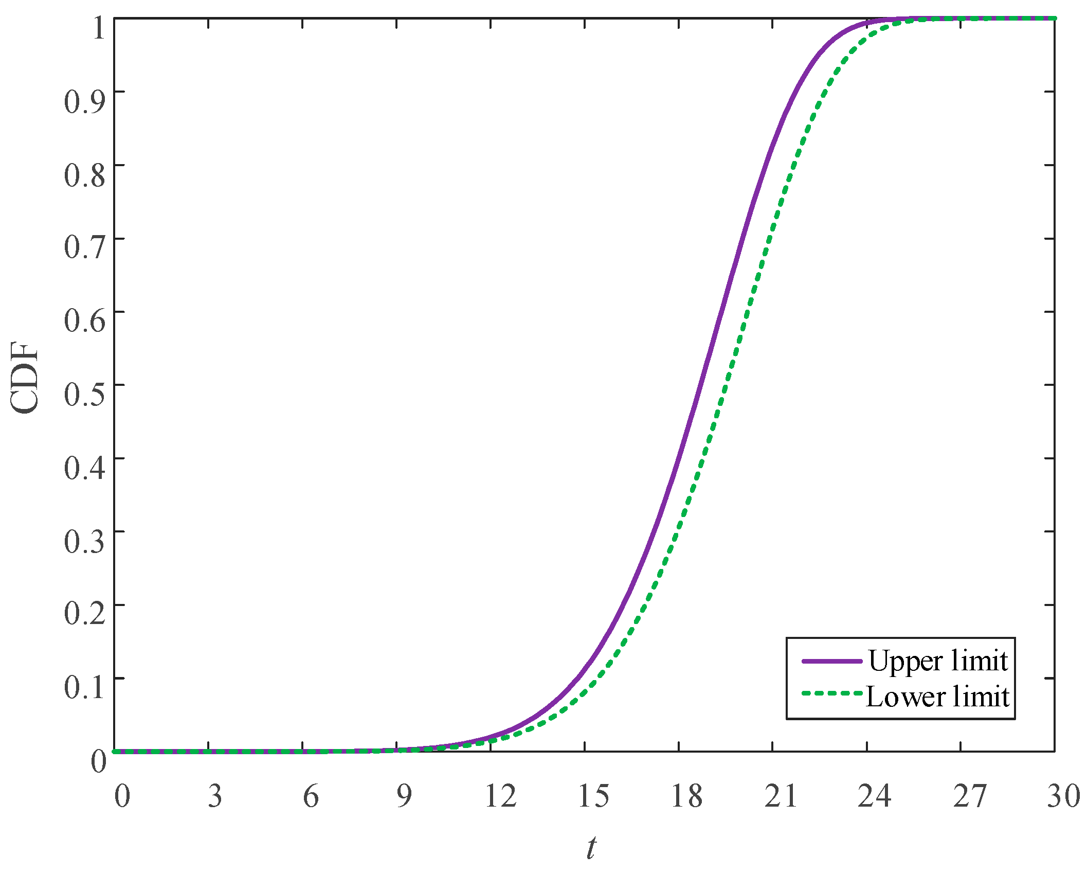
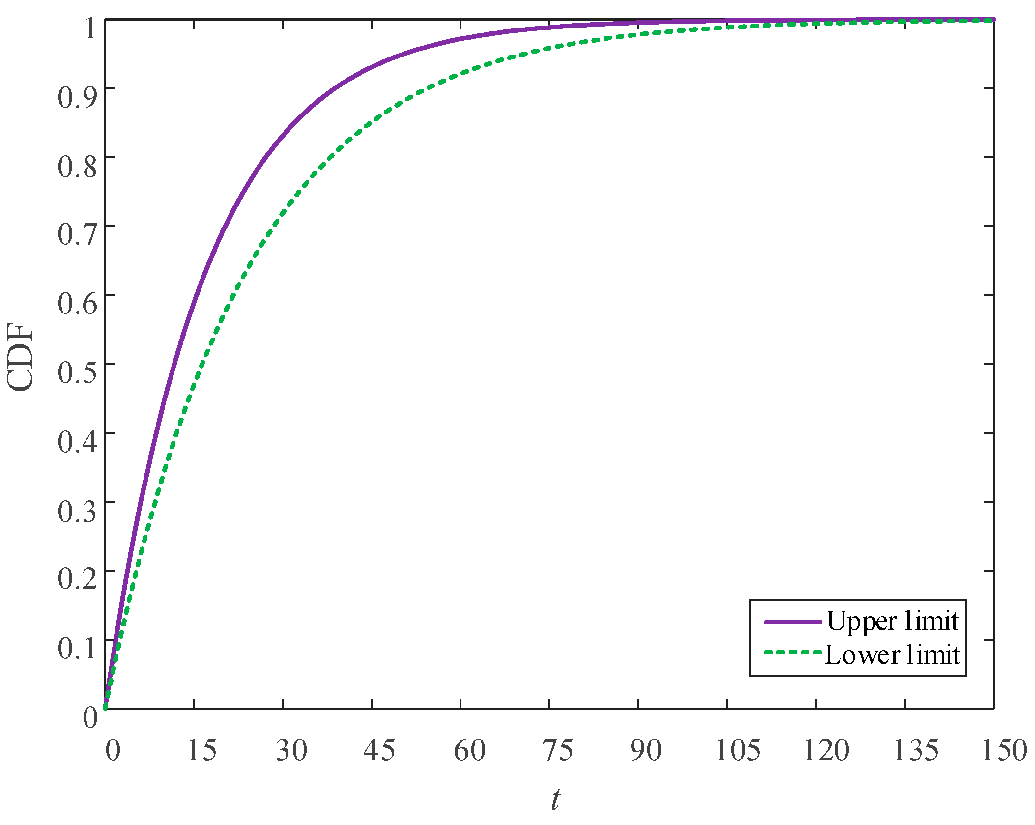
T3	95%	[0.0423, 0.0594]	-	-

. With the distribution parameter intervals, the p-box of T1, T2, and T3 type of components can be obtained, as shown in Figure 2, Figure 3 and Figure 4.

The survival signature of this system can be obtained using Equation (8). The relevant results are shown in

Table 5. Survival signature of the 7 unit system.

l1	l2	l3	l4	Φ(l1,l2,l3,l4)
1	1	0	1	1/2
1	1	0	2	1
1	1	1	1	1
1	1	1	2	1
1	1	2	1	1
1	1	2	2	1
1	2	0	1	1
1	2	0	2	1
1	2	1	1	1
1	2	1	2	1
1	2	2	1	1
1	2	2	2	1

. Since the results of Φ(l₁,l₂,l₃,l₄) = 0 have no effect on the reliability of the system, the corresponding rows are omitted.

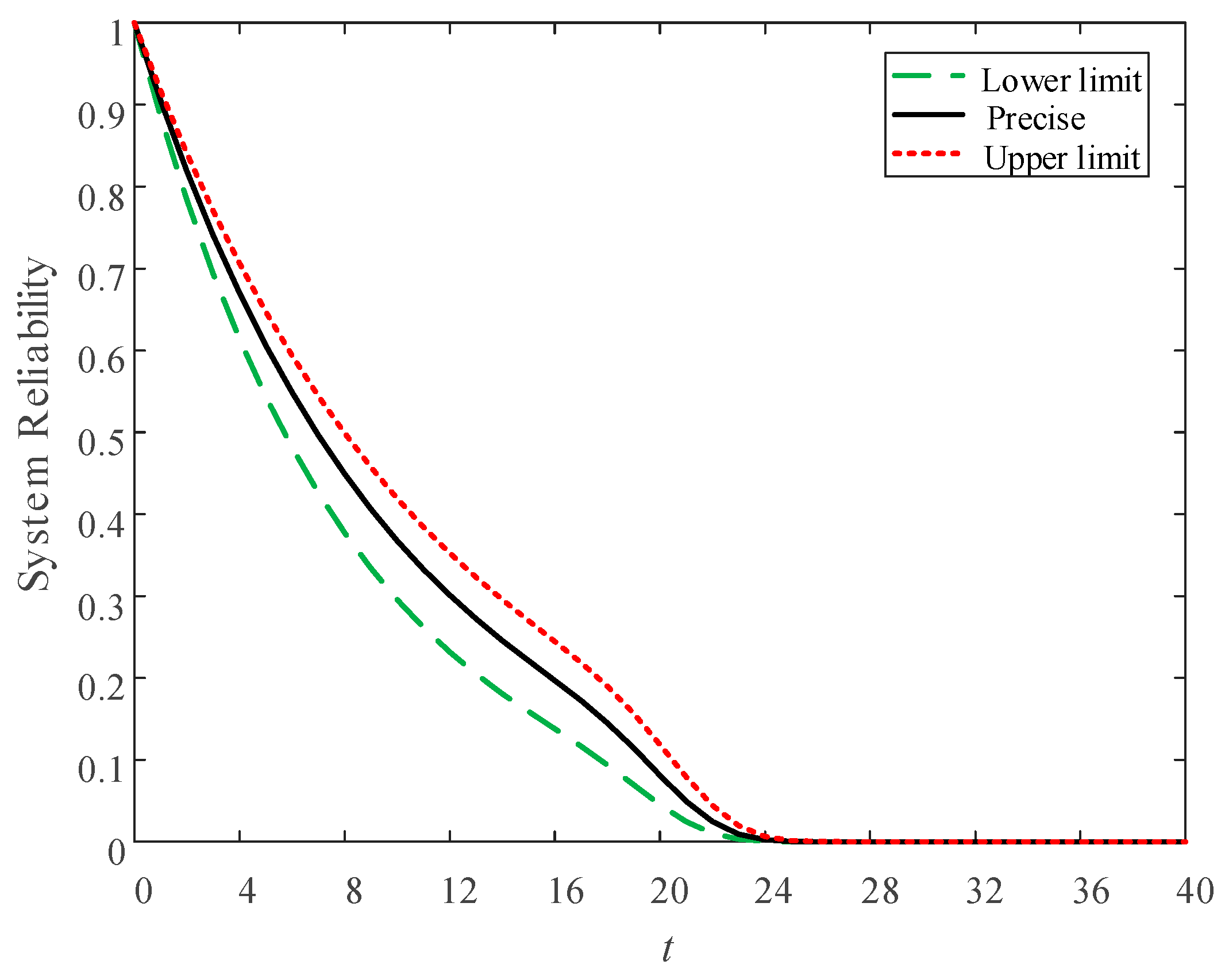
Finally, the lower and upper reliability limit functions of the system can be obtained using Equations (12) and (13). Figure 5 shows the corresponding results. For the purposes of comparison, the precise reliability function of the system is also given in Figure 5.

It can be seen from Figure 5 that the real system reliability is bounded by the lower and upper reliability limits, and the change trend of the limit functions are basically consistent with the true reliability, while the region between them represents the size of the uncertainty. The quantification of system uncertainty helps in effective uncertainty management and increases confidence in the results.

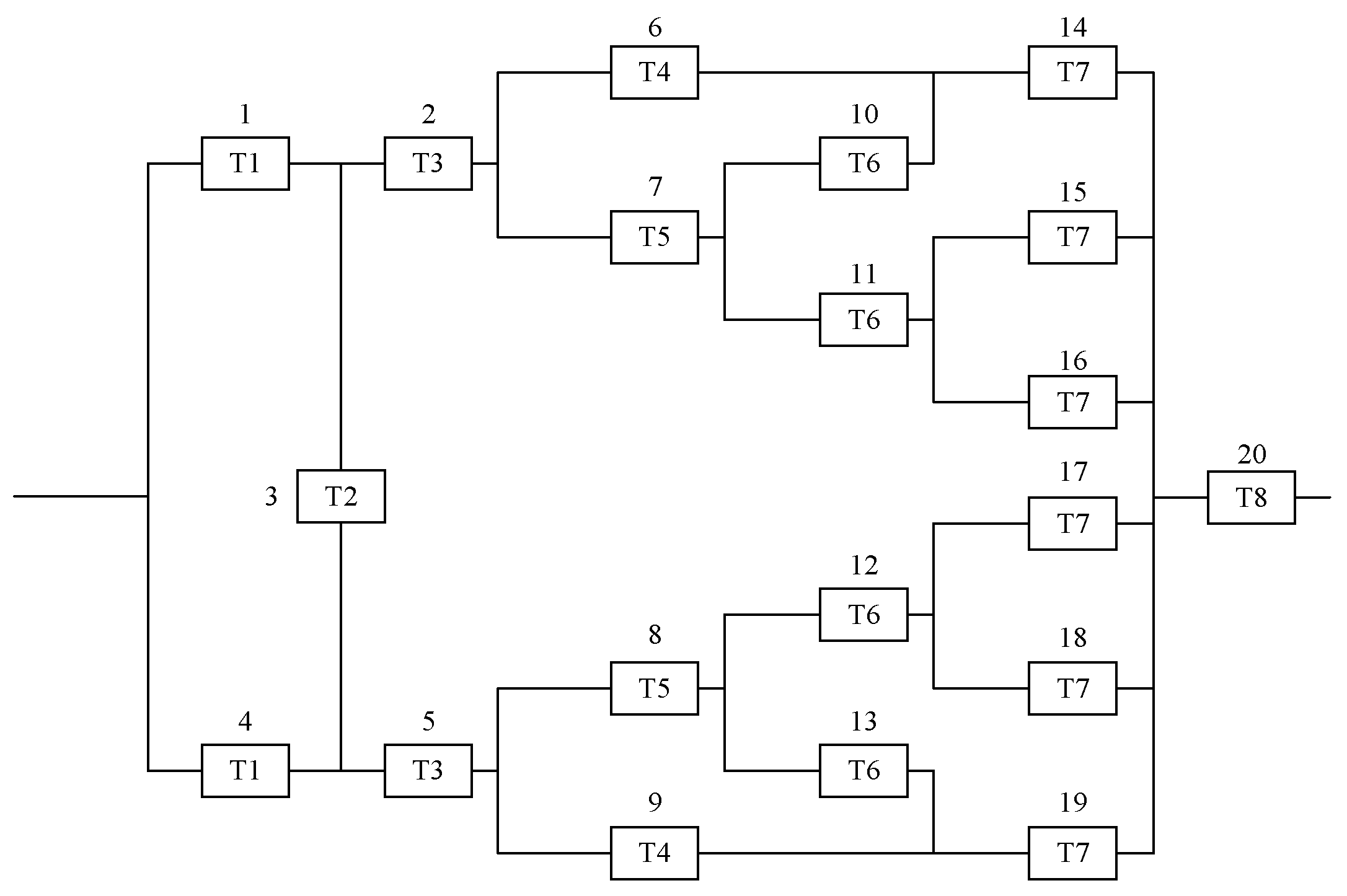
Example 2 (Auxiliary power supply system): In this example, reliability analysis of the auxiliary power supply system for a train is studied based on p-box and survival signature. The reliability block diagram is a complex structure, as shown in Figure 6; the information of each type of component is shown in

Table 6. Information about subsystems or components.

Type	Unit	Distribution	λ	α	β
T1	Pantograph subsystem	Exponential	0.42188	-	-
T2	Insulation subsystem	Exponential	0.16262	-	-
T3	Transformer subsystem	Exponential	0.30944	-	-
T4	Traction converter subsystem 1	Weibull	-	15.0468	7.5118
T5	Traction converter subsystem 2	Exponential	0.14949	-	-
T6	Cable subsystem	Exponential	0.30610	-	-
T7	Single auxiliary converter	Weibull	-	3.8501	2.4975
T8	Power bus	Exponential	0.06572	-	-

. For the exponential distribution, λ represents the failure rate; for the Weibull distribution, α and β represent the scale and shape parameters, respectively. The failure time data the components of types T2, T4, T6, and T8 are shown in

Table 7. Component failure data.

Component Type	Failure Data
T2	0.0349, 0.5847, 1.4434, 2.7405, 3.1757, 3.6475, 3.6797, 5.3652, 6.1297, 7.1585, 7.4751, 8.8711, 11.2241, 12.3072, 15.5112
T4	9.9450, 12.0991, 12.2727, 12.3634, 12.6926, 13.1705, 13.2748, 13.5465, 13.9767, 14.0897, 14.7375, 14.8264, 15.8430, 16.0566, 17.4414
T6	0.1273, 0.3411, 0.4317, 0.4856, 0.7124, 1.0251, 2.2016, 2.2057, 2.3404, 2.4718, 2.5091, 2.9371, 3.9053, 6.1177, 9.3392
T8	0.3468, 0.6107, 1.3017, 1.8569, 3.2337, 3.2970, 7.0740, 7.8945, 8.7717, 14.3528, 15.3607, 17.4318, 19.0361, 21.7302, 26.6873

. Moreover, it is assumed that components of types T1, T3, T5, and T7 have a precise distribution.

Following the steps for calculating the p-box, the 95% Bayesian confidence interval of distribution parameters of type T2, T4, T6, and T8 components are listed in

Table 8. Bayesian parameter confidence interval.

Component Type	Confidence Level	λ	α	β
T2	95%	[0.1384, 0.1940]	-	-
T4	95%	-	[14.8610, 15.5449]	8
T6	95%	[0.2441, 0.3422]	-	-
T8	95%	[0.0636, 0.0892]	-

.

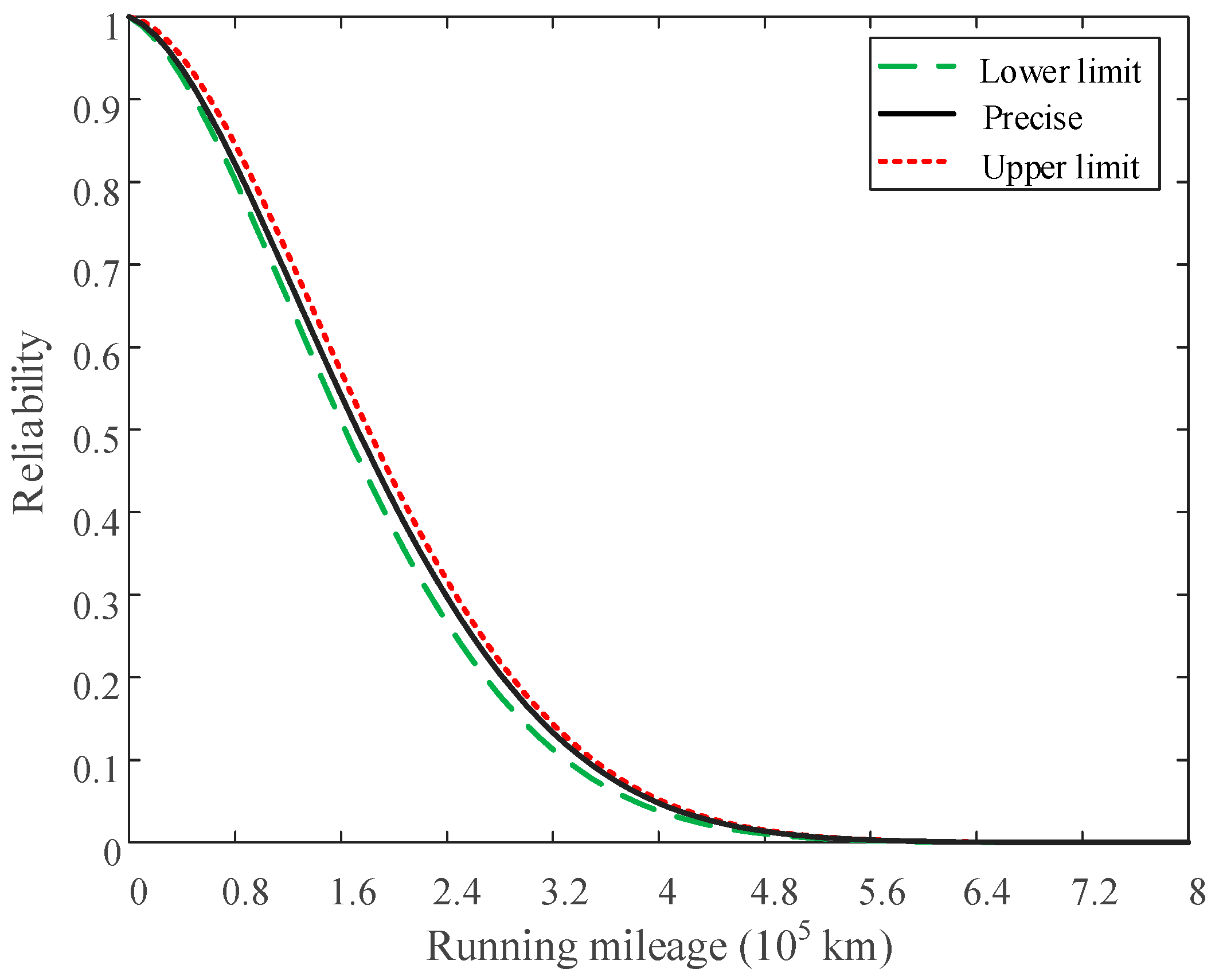
The survival signature of this system can be obtained from Equation (8). Based on p-box and survival signature, the reliability of the system for each point at time t can be obtained from Equations (12) and (13), as shown in Figure 7. Obviously, the change trend of the limit functions are basically consistent with the precise reliability curve, and the quantification of the system uncertainty helps in effective uncertainty management and increases confidence in the results.

5. Conclusions

Modern systems are becoming more and more complicated. At the same time, the exact statistical characteristics of some components may be unavailable because of the limited sample information in practical engineering. The lack of information about a true form of life distribution leads to the presence of epistemic uncertainty over the distributional parameters (e.g., mean and variance). Previous analyses have shown that, if epistemic uncertainty is not taken into account during reliability prediction, the results may be seriously biased and fail to give a useful and reliable estimate. Therefore, it is increasingly important to propose a methodology for reliability assessment of complex systems under aleatory and epistemic uncertainties.

In this paper, an efficient and effective method for reliability analysis of complex systems is proposed based on the theories of p-box and survival signature. Bayesian inference is used to construct the p-boxes and the life distributions of the components with a limited number of samples. The theory of survival signature is applied to calculate the reliability of the system with a mixture of precise and imprecise knowledge of the life distributions of the components. The epistemic uncertainty contained in the system is effectively quantified by using the theory of p-box. Furthermore, reliability analysis of a system using survival signature could separate the system structure from the component probabilistic failure distribution. Therefore, the proposed approach is easy to be implemented in practice and has high computational efficiency.

It should be noted that, because we calculated the p-box based on Bayesian interval estimation in this paper, we need to know the lifetime distribution types of the components. In reality, we may obtain prior information of lifetime distributions of the components from different sources, such as expert experience, failure data, engineering knowledge, etc. How to give a reasonable prior for Bayesian interval estimation using these information sources is a topic of future research for the authors. In general, however, based on p-box and survival signature, this paper presents a new and practical method for system reliability analysis with limited samples, which quantifies the uncertainty in system reliability analysis effectively.