Independent Analysis of Decelerations and Resting Periods through CEEMDAN and Spectral-Based Feature Extraction Improves Cardiotocographic Assessment

Abstract

Fetal monitoring is commonly based on the joint recording of the fetal heart rate (FHR) and uterine contraction signals obtained with a cardiotocograph (CTG). Unfortunately, CTG analysis is difficult, and the interpretation problems are mainly associated with the analysis of FHR decelerations. From that perspective, several approaches have been proposed to improve its analysis; however, the results obtained are not satisfactory enough for their implementation in clinical practice. Current clinical research indicates that a correct CTG assessment requires a good understanding of the fetal compensatory mechanisms. In previous works, we have shown that the complete ensemble empirical mode decomposition with adaptive noise, in combination with time-varying autoregressive modeling, may be useful for the analysis of those characteristics. In this work, based on this methodology, we propose to analyze the FHR deceleration episodes separately. The main hypothesis is that the proposed feature extraction strategy applied separately to the complete signal, deceleration episodes, and resting periods (between contractions), improves the CTG classification performance compared with the analysis of only the complete signal. Results reveal that by considering the complete signal, the classification performance achieved 81.7% quality. Then, including information extracted from resting periods, it improved to 83.2%.

1. Introduction

During labor and delivery, the main aim of fetal monitoring is to identify potential hypoxic fetuses to prevent adverse outcomes. In current clinical practice, this operation is commonly performed by using an instrument known as the cardiotocograph (CTG), which provides the information corresponding to the fetal heart rate (FHR) and uterine contraction (UC) activity. Clinicians visually examine these recordings based on several morphological signal patterns defined in medical guidelines [1,2,3]. Unfortunately, CTG interpretation by this methodology has shown serious disadvantages, such as extensive intra- and inter-observer disagreement, which lead to poor interpretation objectivity and reproducibility [4,5,6].

That is why several approaches have been proposed to provide more representative information about fetal health status. Particularly, in the signal processing field, many studies have focused on extracting hidden FHR characteristics that can improve the CTG interpretation. However, despite these efforts, the results obtained are not satisfactory enough for their use in clinical practice so far [5,7,8,9].

On the one hand, current advances in medical research indicate that a correct assessment of fetal distress requires a good understanding of the compensatory mechanism of the fetus. Besides, its health depends on how it compensates itself under certain stimuli, such as UC events, over time. These compensatory mechanisms are controlled by the autonomic nervous system (ANS), which modulates the fetal cardiac activity after a perceived oxygen insufficiency [10,11]. Indeed, the fetal compensation response, represented by variations in the beat-to-beat FHR, can involve important time-variant dynamics related to the fetal condition [12,13]. Given that concept, an appropriate FHR signal analysis should consider the nonlinear and non-stationary characteristics of the compensatory mechanism. Therefore, conventional signal processing methods that do not integrate these characteristics could not be suited for a correct CTG analysis.

On the other hand, according to the literature [14], the CTG interpretation problems are mainly associated with the assessment of FHR decelerations, which are certainly fetal cardiac responses modulated by the ANS [6]. Likewise, recent research in biomedical engineering indicates that the UC activity has a graded effect on the FHR response [15,16].

In this context, different signal processing approaches have been proposed, which are mainly based on frequency-domain, nonlinear feature extraction, and time-variant analysis. However, considering the physiological phenomena explained above, they have certain limitations because most of the proposed approaches focus only on fetal reactivity as a response to a UC event, without considering the time-variant characteristics involved in the modulated FHR response over time.

In previous works, we have shown that using the complete ensemble empirical mode decomposition with adaptive noise (CEEMDAN) in combination with time-varying autoregressive (TV-AR) modeling, might be useful for the analysis of those physiological characteristics [17,18]. Firstly, CEEMDAN, as an appropriate tool for decomposing nonlinear and non-stationary signals, can help to demodulate the FHR signal dynamics modulated by the ANS (dynamics of interest). This technique depends on the direct extraction of the energy associated with the signal oscillations, and its operation provides a finite number of intrinsic mode functions (IMFs). Secondly, the IMFs are analyzed in the spectral-domain by using TV-AR spectral-based analysis, which allows tracking the time-varying frequency components involved in each IMF, independently.

Based on this feature extraction methodology, this work focuses on studying the CTG classification performance by considering the complete FHR signal, deceleration episodes, and resting periods (between contractions) separately. Considering that recent research has shown that a separate analysis of these FHR signal segments can improve the detection of fetal distress [19], we propose to extract information from those segments independently and determine their contribution in CTG analysis evaluated by a support vector machine (SVM) based classification. The main hypothesis is that the feature extraction approach based on CEEMDAN and TV-AR modeling, applied separately to the complete signal, deceleration episodes, and resting periods, improves the CTG classification performance compared with the traditional analysis based only on the complete signal.

The rest of the paper first presents a brief overview of related works in the field of FHR signal feature extraction (Section 2). Then, Section 3 explains the methodology and describes, in detail, the signal processing techniques used for the CTG signal analysis. Continuing, Section 4 presents a comprehensive analysis and foundations behind the feature extraction operation and the strategy used for their evaluation. Finally, Section 5 concludes this paper and discuses perspectives for future work.

2. State of the Art

2.1. Analysis in Frequency-Domain

According to the literature [20,21,22], the FHR signal involves information of interest that lies in different frequency bands. A continues component corresponds to the FHR signal average. A very low frequency (VLF) band (≤0.03 Hz) that involves slow signal dynamics is related to the nonlinear morphological behavior of FHR decelerations and accelerations. A low frequency (LF) band (0.03–0.15 Hz) is mainly associated with fetal sympathetic ANS activity. A medium frequency (MF) band (0.15–0.5 Hz) is related to the fetal movements and breathing of the mother. Finally, a high frequency (HF) band (0.5–1.0 Hz) is related to fetal breathing.

Given the above, different approaches have been proposed to extract information from such frequency bands of interest. Most of them depend on spectral-based operations because it is assumed that variations in the frequency-domain can be related to the fetus’s condition [23]. In general, these methods are based on fast Fourier transform (FFT) [20,24,25,26,27,28,29], and AR spectral-based analysis, which allows the extraction of quantitative spectral parameters [30,31,32].

2.2. Nonlinear Features

Several techniques have been proposed to study the nonlinear characteristics involved in the FHR signal in relation to fetal health status. In this context, mutual information (MI) has been employed to design efficient features for FHR signal analysis [33] and study the UC and FHR coupling [34]. Multivariate analysis based on linear and nonlinear features has been proposed to discriminate between normal and intrauterine growth-restricted fetuses [35]. Multiscale entropy (MSE) has been used to estimate the signal complexity [36,37] and regularity [38] of FHR recordings. Besides, as presented in Section 3.2.3, empirical mode decomposition (EMD) has been used in different approaches proposed for CTG signal analysis.

2.3. Time-Variant Techniques

Most of the time-variant approaches are based on short time Fourier transform [39], quadratic time-frequency distributions [40], and TV-AR modeling [13,22,41]. Besides, continuous wavelet transform has been used for a spectral-based analysis of the FHR and UC signals [42], and discrete wavelet transform has been employed to study the transient behavior of the UC events [43].

3. Methodology

This work proposes to study the FHR signal characteristics with a focus on the dynamics resulting from ANS modulation. The main idea is to extract signal features from the entire signal, during decelerations and resting periods, thereby investigating whether by analyzing such FHR signal segments separately, the CTG classification can improve compared with the traditional analysis based on the entire signal.

After a perceived oxygen insufficiency, as a first fetal response, the sympathetic nerves may act as a compensatory mechanism to improve the fetal heart-pumping activity, whereas the parasympathetic ANS activity may decrease [24,44]. In contrast, after the perceived threat (oxygen insufficiency) has been attenuated, the parasympathetic ANS may be activated, and the sympathetic activity decreases. That interaction is a normal phenomenon; however, in some cases, these physiological mechanisms may be weakened, leading to fetal distress. Besides, in fetuses, the sympathetic ANS system predominates, because it develops earlier than the parasympathetic ANS system, which becomes more developed with advancing maturity [29]. Therefore, the main goal of our work, as several related approaches proposed in the literature [26,39,45], was to extract information from an FHR signal related to the sympathetic ANS activity in order to estimate a fetus’s state of health.

As explained above, the FHR data involves highly complex characteristics mainly associated with their nonlinear and non-stationary behavior as a result of the ANS activity [11]. Therefore, it is reasonable to think that if such characteristics are not previously demodulated or decomposed, the extraction of the information of interest could be a difficult task. On the other hand, conventional signal processing methods can no longer be used for the analysis of those characteristics, because they are not appropriate to describe this time-variant physiological phenomenon.

In this context, we propose an approach that combines two signal processing techniques: CEEMDAN [46] and TV-AR modeling [47] for the analysis in the time- and spectral-domain, respectively.

On the one hand, CEEMDAN is an adaptive technique that allows decomposing non-stationary and nonlinear time series into IMFs, which are computed by the direct extraction of the energy associated with the signal oscillations. The CEEMDAN decomposition operation is based on similar principles of signal demodulation in amplitude; therefore, we postulate that this method can be useful for extracting the information of interest involved in the FHR dynamics as a result of the ANS modulation. Consequently, the main advantage of CEEMDAN is its dependency on the data-driven mechanism, which does not require a priori known bases as in the case of other traditional techniques such as wavelet and FFT-based decomposition [48,49,50,51].

On the other hand, in order to examine the frequency information involved in the IMFs, we employ TV-AR spectral-based analysis. It is a technique for time series analysis based on a mathematical model fitted to a sampled signal. Therefore, it has several advantages for the analysis of the FHR signal because this model provides a signal description that makes it easier to analyze by a few model parameters. Besides, it allows the extraction of quantitative time-dependent spectral parameters, which are better suited for quantitative analysis [32]. In the spectral-domain, the information of interest involved in the IMFs is represented by the power spectral density peaks, which represents the contributions of their time-variant frequency components. Additionally, considering that the sampling frequency of the FHR signals we studied was the only 4 Hz, the AR modeling was appropriate for the IMF, spectral-based analysis. The AR modeling method effectively describes the peaks of a narrow-band power spectrum [52], and it requires only a fraction of the signal samples that are needed by standard methods, such as the FFT, in order to obtain the same spectral resolution.

In summary, the IMFs computed by the CEEMDAN allow obtaining a less complex signal better suited for parametrical modeling, such as TV-AR modeling. As a result, tracking the FHR frequency components of interest is now an easier task because the spectral analysis focuses on tracking only one main frequency component of interest for each IMF over time.

The proposed CTG signal feature extraction strategy is presented in Figure 1. In this figure, the diagram blocks represent the main processing steps applied to the CTG recording, which are explained in detail in Section 3.1, Section 3.2 and Section 3.3. The codes and machine learning techniques used for the approach we propose were implemented in Matlab^® environment version 2018b.

3.1. CTG Recordings Dataset

The proposed analysis was performed using real CTG data extracted from the CTU-UHB database [53], which contains 552 recordings of FHR and UC signals, both sampled at 4 Hz. From this database, we selected a CTG dataset consisting of two groups: normal and acidotic, based on the pH and BDecf (base deficit in the extracellular fluid) outcome parameters. According to the literature [54], at birth, values of pH > 7.20 and BDecf < 12 commonly indicate a normal condition, whereas pH < 7.05 and BDecf ≥ 12 can indicate a fetal metabolic acidosis. Based on these class formation criteria, our dataset consisted of 372 recordings, 18 labeled as acidotic, and 354 labeled as normal fetuses.

3.2. CTG Signal Analysis

This section presents the signal processing strategy applied to the CTG signal, whose principles are explained using the CTG recording shown in Figure 2. These FHR and UC signals correspond to the last 1500 s of the recording number 1179 extracted from the CTU-UHB database.

3.2.1. Signal Preprocessing

The CTG signal can involve different types of artifacts, such as loss of data and outliers, which are mainly generated by the loss of the sensor’s contact because of movements that can temporarily interrupt the signal’s acquisition.

On the one hand, for the FHR signal preprocessing, we apply the artifact rejection method proposed in [55]. First, the signal values considered physiologically inconsistent, i.e., outside the range between 50 bpm and 210 bpm, are removed from the signal. Then, loss-of-signal data ≤75 s in length are interpolated by using a Hermite spline method.

On the other hand, for the UC signal, loss-of-signal data less than 25 s in length are interpolated; then, the signal is filtered by a moving average filter of 15 s windows length. This filtered UC signal is using for the deceleration identification, as explained in Section 3.3. The preprocessed FHR and UC signals are shown in Figure 3a,b, respectively.

3.2.2. FHR Signal Detrending

After the preprocessing step, and before the CEEMDAN decomposition operation, a signal detrending operation is applied. For this purpose, we first compute a VLF signal trend denoted as the floating-line. The floating-line allows tracking the morphological behavior of FHR decelerations and accelerations, whose behavior involves nonlinear characteristics [5,50]. Following [56], this floating-line is computed by a median filter with a sliding window of 10 s length, whose size was determined as follows:

• We randomly selected a set of ten CTG recordings from the CTU-UHB database.
• Each FHR signal was filtered by a median filter using different window lengths in the range of 6 to 12 s in steps of 1 s.
• The extracted traces (seven for each signal) were superimposed on the corresponding raw FHR signal in order to examine which one tracks the FHR decelerations and accelerations better.
• After a visual analysis, we selected the trace computed by a sliding window of 10 s length.

The computed floating-line is shown in Figure 4a in red. Once the floating-line is computed, it is subtracted from the FHR signal, whose resulting signal (detrended FHR signal) is shown in Figure 4b. For the subsequent decomposition and spectral analysis, the detrended FHR signal is used.

3.2.3. FHR Signal Decomposition and TV-AR Spectrum Computation

As mentioned above, the FHR signal decomposition is performed by the CEEMDAN method. The empirical mode decomposition (EMD) [48], which corresponds to a previous version of this technique, has been used in different biomedical engineering approaches [49]. Particularly, in FHR signal analysis it has been used for FHR estimation from Doppler Ultrasound signals [57], analysis of the FHR signal components in order test the reliability of the EMD performance [58], FHR baseline estimation with analysis of fetal movements [59], assessment of the high frequency FHR information [60], enhancement of the CTG signal quality by reducing signal artifacts [50], and FHR signal feature extraction and classification [49,61]. These works have concluded that EMD could be appropriate for the analysis of the FHR signal components in the time-domain.

Since EMD was proposed [48], it has developed to overcome different problems associated with the decomposition [46,62,63]. The main issue involved in the original EMD method is the mode mixing; i.e., more than one mode of oscillation may contribute to one IMF, or one mode can spread across different IMFs. In consequence, it can lead to an unreliable decomposition of the FHR signal because the IMFs may not correctly describe the FHR signal dynamics of interest. In order to solve this issue, in [46], the improve complete ensemble empirical mode decomposition with adaptive noise (CEEMDAN) method has been proposed. This updated version solves the described mode mixing problem and subsequent drawbacks, such as residual noise and spurious modes generated by the operation itself. Therefore, in this work, we performed the FHR signal decomposition based on the CEEMDAN method. Following [61], the IMFs were computed by using a noise standard deviation (Nstd) set to 0.03, and both the number realizations (NR) and the maximum number of sifting iterations (NI) were set to 50. For a more in-depth explanation of CEEMDAN, please refer to [46]. Once the FHR signal is decomposed, the spectral analysis is performed for each IMF individually.

As explained at the beginning of Section 3, the stationary version of AR modeling has been studied in several approaches, and revealed different advantages compared with non-parametric, spectral-based methods [64].

An AR model assumes that the signal value $y[n]$ at the current sample number n in a data sequence $y[1],y[2],\dots ,y[N]$ can be modeled in function of the p most recent sample values $y[n-1],y[n-2],\dots ,y[n-p]$, and a Gaussian white zero-mean noise $e[n]$ of variance ${\sigma }^2$ as presented in Equation (2). In this equation, p corresponds to the model order, whose value is generally much smaller than the sequence length N, $a_k\{k=1,2,\dots ,p\}$ are the stationary AR coefficients, and n is the discrete-time index.

$$y[n]=-{\displaystyle \sum _{k=1}^p}{a}_{k}y[n-k]+e[n]$$

(1)

Considering that the AR model is applied for each IMF, Equation (1) can be expressed as presented in Equation (2), where i represents the index number of the computed IMFs.

$${\mathrm{IMF}}_i[n]=-{\displaystyle \sum _{k=1}^p}{a}_{i,k}{\mathrm{IMF}}_i[n-k]+e[n]$$

(2)

The z-transform can be applied to Equation (2), whose resulting model transfer function is presented in Equation (3). Here, $IM{F}_i[z]$ and $E[z]$ are the z-transforms of the time series IMF_i[n] and the noise $e[n]$, respectively.

$$H_i[z]=\frac{IM{F}_i[z]}{E[z]}=\frac{1}{1+{\sum }_{k=1}^p{a}_{i,k}{z}^{-k}}.$$

(3)

Then, the stationary AR spectrum can be computed by evaluating $H_i[z]$ around the unit circle in the complex plane; i.e., $z=e^{j2\pi f}$:

$$SA{R}_i(f)=\frac{{\sigma }^2}{{\left|1+{\sum }_{k=1}^p{a}_{i,k}{e}^{-j2\pi fk}\right|}^2}.$$

(4)

Considering that the phenomenon of focus involves dynamics strongly variant time, stationary AR modeling [47] is no longer suitable for the analysis. For this reason, we employ TV-AR modeling as an appropriate method for the proposed spectral analysis. A representation of this time-varying version is presented in Equation (5), where $a_{i,k}(n)\{k=1,2,\dots ,p\}$ are now the time-dependent coefficients, whose set of values $a_{i,k}$ is updated sample-by-sample n.

$${\mathrm{IMF}}_i[n]=-{\displaystyle \sum _{k=1}^p}{a}_{i,k}(n){\mathrm{IMF}}_i[n-k]+e[n].$$

(5)

Likewise, this operation results in a time-varying AR model transfer function, which is represented by:

$$H_i[z,n]=\frac{IM{F}_i[z,n]}{E[z,n]}=\frac{1}{1+{\sum }_{k=1}^p{a}_{i,k}(n)z^{-k}}.$$

(6)

Analogously, the time-varying version of the AR spectrum presented in Equation (4) can be described by:

$$SA{R}_i(f,n)=\frac{{\sigma }^2}{{\left|1+{\sum }_{k=1}^p{a}_{i,k}(n)e^{-j2\pi fk}\right|}^2}.$$

(7)

This last equation allows performing the proposed time-varying analysis, because the computed spectrum resultantly depends on frequency as well as on time.

Following [13], in this work, the AR coefficients ($a_k(n)$) were computed by using a recursive least squares algorithm with a forgetting factor ($\lambda$). The forgetting factor is a model parameter related to the memory time considered in the studied process. Therefore, considering that our approach focuses on the analysis of the same physiological phenomenon as in [13] (analysis of fetal ANS activity over time), we decided to use the same forgetting factor set to 0.99.

For the selection of a suited model order p, we first considered the characteristics of the IMFs. An IMF corresponds to a non-overlapping function modulated in amplitude and frequency [46]. Given that concept, we assumed that in the frequency-domain, for each IMF, only one main frequency component contained the information of interest over time; i.e., in the AR spectrum, only one absolute maximum peak involved such information at each sample n. With this in mind, we studied a set of thirty IMFs (selected randomly from different FHR signals extracted from the database). For each selected IMF, the AR spectrum was computed by using different AR model orders in the range of 4th and 10th. Then, we examined which order p offers a better spectral representation of the frequency component of interest, taking into account that only one main component should be clearly distinguished. After a visual analysis, and following [18], we decided to use a 6th AR model order p.

Examples of the CEEMDAN and TV-AR spectrum computation are shown in Figure 5, in the left and right columns, respectively. This example was obtained by the decomposition of the detrended FHR signal presented in Figure 4b. The TV-AR spectrum is represented by a color map, where the lowest and highest energy level are shown in blue and yellow, respectively. Additionally, for better visualization of the spectral dynamics, the energy values have been normalized between 0 and 1 for each sample n. In addition to the time-varying spectral representation, we computed the average of the TV-AR spectrum (right column), which illustrates the frequency band involved for each IMF.

It is important to note that the number of IMFs obtained from the 372 signals of the dataset (see Section 3.1) varies from 12 to 17. Nevertheless, based on the spectral information described above (averaged TV-AR spectrum), we decided to study the first ten IMFs, thereby considering the entire FHR frequency band of interest.

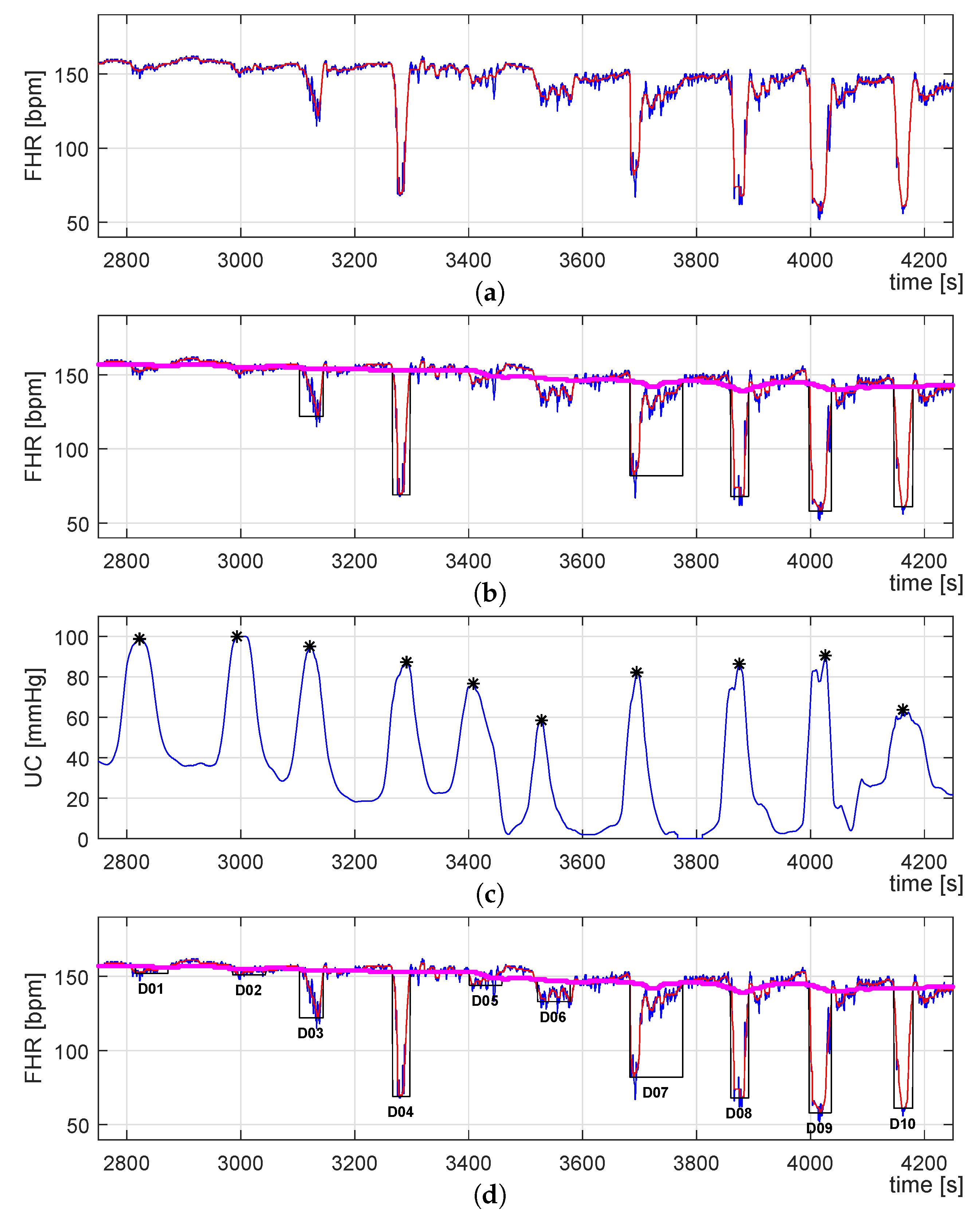
3.3. Identification of UC-Deceleration Episodes

As explained at the beginning of Section 3, the main purpose of this work was to investigate whether, by separately analyzing the complete signal (CS), during decelerations (DD), and during resting (DR) periods, the CTG classification could improve compared with analyzing only the complete signal. Therefore, it is necessary to identify the FHR decelerations in order to differentiate them from the resting periods. The method proposed for deceleration identification is explained using the signals presented in Figure 6a, which correspond to the preprocessed FHR signal and floating-line computed in Section 3.2.2.

For the deceleration episodes’ identification, we propose a new concept: the UC-deceleration episodes. This concept not only considers evident decelerations as defined in guidelines (>15 bpm in amplitude and >15 s length) [1] but also considers the UCs as stimuli that excite a fetal response.

Following [56], the identification of UC-deceleration episodes is performed in two steps. First, evident deceleration episodes are detected by using the floating-line (described in Section 3.2.2) and a progressive baseline (described below). Then, episodes that were not recognized in the previous step are identified considering the UCs stimuli.

In the first step, we propose computing a progressive baseline (PBL), which allows recognizing evident deceleration episodes. This proposed PBL is computed as follows:

• A virtual baseline (VBL) is estimated by filtering the FHR signal using the same median filter for the floating-line computation but with a different sliding window. Following [65], the sliding window size was set to 400 s length.
• Then, the VBL allows defining a range in amplitude delimit by the low (L) and high (H) traces, which corresponds to the signal data that will be considered for the PBL computation. These traces are described by Equations (8) and (9), where n corresponds to the sample number, and $\Delta$FHR is set to 10 bpm following [66].

  $$L(n)=\mathrm{VBL}(n)-\Delta \mathrm{FHR}.$$

  (8)

  $$H(n)=\mathrm{VBL}(n)+\Delta \mathrm{FHR}.$$

  (9)
• Finally, the PBL is computed by considering only the data described by FHR_LH (see Equation (10)) by using the same median filter used for the VBL extraction.

  $${\mathrm{FHR}}_{LH}(n)=\left\{\begin{array}{cc}L(n)\hfill & \mathrm{FHR}(n)<L(n)\hfill \\ \mathrm{FHR}(n)\hfill & L(n)\le \mathrm{FHR}(n)\le H(n)\hfill \\ H(n)\hfill & \mathrm{FHR}(n)>H(n).\hfill \end{array}\right.$$

  (10)

For the evident decelerations’ detection, the PBL is used as a threshold over the floating-line. Differences of more than 15 bpm in amplitude and more than 15 s length [1] are detected as evident decelerations. The computed PBL and evident deceleration episodes are plotted in Figure 6b in magenta and black, respectively.

The second step allows the identification of the episodes that were not recognized as evident decelerations, but that are certainly response to UC events. These episodes, also called $UC$-$segments$, are defined following the criteria proposed in [13], which correspond to FHR signal segments starting 7 s before a UC apex and ending 50 s after it. First, UC apexes of significant amplitude (i.e., ≥30 mmHg) are detected and considered for this operation. Figure 6c shows the preprocessed UC signal (described in Section 3.2.1) and the detected UC apexes. Then, when an evident deceleration was not recognized, but a UC apex was detected, its corresponding uc-segment was added to be considered for the analysis. The complete set of uc-deceleration episodes is presented in Figure 6d. Here, we can observe that episodes D01, D02, D05, and D06, which were not recognized as evident decelerations, were included in this second identification step.

4. Evaluation and Results

Making use of the techniques presented in the previous section, we proceed to evaluate our approach. As explained in Section 1, this work proposes extracting information from the CTG signal based on CEEMDAN and TV-AR modeling, whose feature extraction operation is performed separately on the complete FHR signal, deceleration episodes, and resting periods. The main idea is to determine whether by considering those segments independently, the CTG classification performance can improve compared with the traditional analysis based only on the complete signal.

In this Section, we first explain the foundation of the proposed signal features qualitatively. Then, we present the results concerning their performance in CTG analysis by using a SVM based classification.

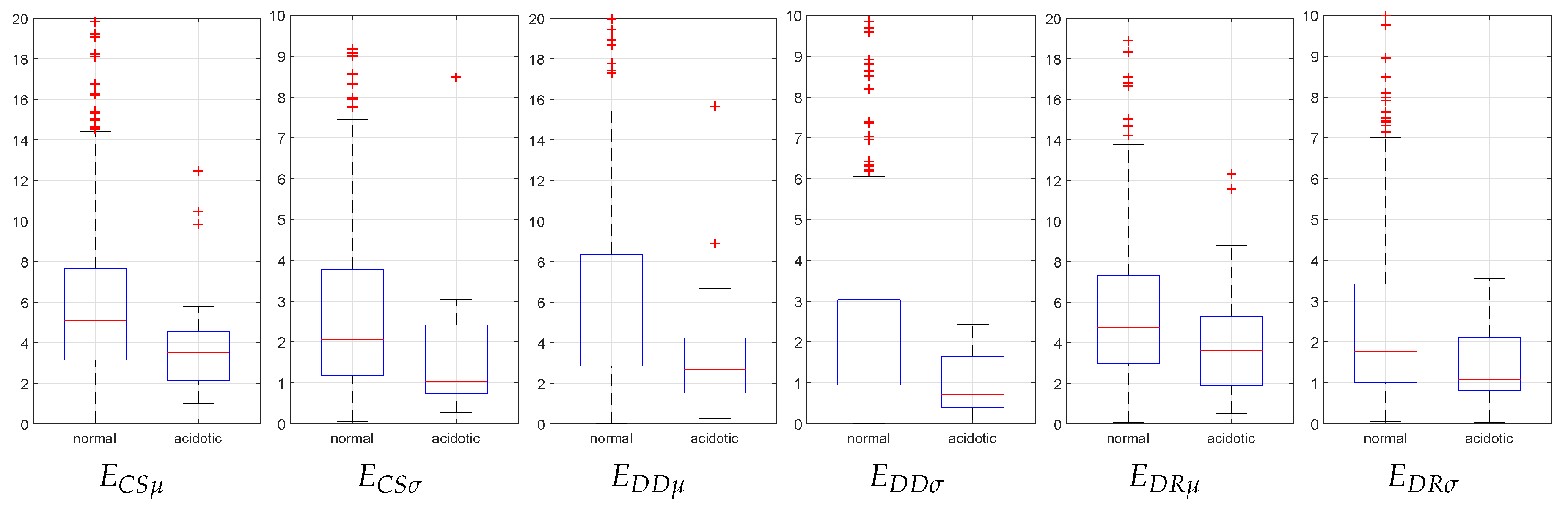
4.1. Definition of Proposed Features

This section presents a comprehensive analysis behind the extraction of the proposed features, whose explanation is performed using two representative cases extracted from the dataset described in Section 3.1. These cases are presented in Figure 7, which belong to the recording numbers 1189 (left column) and 2011 (right column) of the CTG database, as examples of normal and acidotic conditions, respectively. Figure 7a,b shows the raw FHR signal of each recording. The second row shows the preprocessed FHR signal (blue), computed PBL (magenta), floating-line (red), and the identified deceleration episodes (black). The third and fourth row shows the detrended FHR signal and the IMF₆, which was arbitrarily selected for the explanation of the proposed spectral analysis. This IMF involves spectral dynamics in the frequency range between 0.03 and 0.15 Hz (see Figure 5), whose band, as explained in Section 2.1, is mainly related to the fetal sympathetic ANS activity. The fifth and sixth rows show the TV-AR spectrum computed from the IMF₆ and its corresponding total energy (E), respectively. The total spectral energy E is calculated in the complete band of interest (0–2 Hz) for each time instant n, as described in Equation (11). For better visualization and comparison of these two examples, the spectral energy values were scaled between 0 and 100 with respect to the maximum value of energy of these indicators. Besides, in the third, fourth, and sixth rows, the deceleration episodes are highlighted in gray. It is important to mention that the data normalization explained above was performed only for a better explanation of this example. For the feature computation and evaluation, as presented in Section 4.2, the features were standardized using z-score based normalization.

It is important to note that for the graphic explanation of the proposed spectral analysis, only one IMF was considered. Nevertheless, for the subsequent feature extraction operation (performed in Section 4.2), the entire FHR frequency range of interest was considered by analyzing the first ten IMFs, as explained in Section 3.2.3.

$$E[n]={\displaystyle \sum _{f=0}^{2Hz}}(SAR[f,n]).$$

(11)

Results shown in Figure 7i,j indicates that the representative examples exhibit important spectral dynamics strongly variant in time. As represented by the spectral energy E (last row), the spectral behavior differs between the normal and the acidotic case. Notably, for the normal case, the indicator E (see Figure 7k) presents pronounced variations in amplitude. In contrast, the example corresponding to an acidotic fetal condition shows completely different behavior. In this acidotic case, E is considerably lower and exhibits a less marked variation in amplitude compared with the previous case. This phenomenon can be directly related to the fetal health status because the fetal response, modulated by the sympathetic ANS activity, may decrease for an acidotic case [13].

In order to evaluate whether those graphic observations are related to the fetal health condition, we compute the indicator E for the complete dataset (defined in Section 3.1). Then, from each obtained indicator, we calculate two statistical coefficients: the average ($\mu$) and the standard deviation ($\sigma$). It is important to note that for this example, only two features were computed; nevertheless, as explained in Section 4.2, for the evaluation of our approach, a larger set of features was extracted. Finally, we apply a Wilcoxon rank-sum test [67], which allows determining whether such extracted features are statistically significant (p-value < 0.05) under the hypothesis that the median value of normal class data differs from the median value of the acidotic class data.

The previous operation was performed independently for the complete signal ($E_{CS}$), during decelerations ($E_{DD}$), and during resting periods ($E_{DR}$).

Table 1. Results of the statistical test for the extracted spectral features for the complete signal (CS), during decelerations (DD), and during resting (DR) periods, whose values correspond to the 50th[25th–75th] percentiles of the data, respectively.

Feature	Normal Cases	Acidotic Cases	Significance (p-Value)
$E_{CS\mu }$	$5.09[3.14-7.66]$	$3.50[2.14-4.56]$	0.0213
$E_{CS\sigma }$	$2.06[1.18-3.78]$	$1.03[0.74-2.42]$	0.0079
$E_{DD\mu }$	$4.87[2.85-8.35]$	$2.67[1.52-4.22]$	0.0016
$E_{DD\sigma }$	$1.69[0.95-3.03]$	$0.72[0.39-1.64]$	0.0015
$E_{DR\mu }$	$4.76[2.98-7.31]$	$3.63[1.90-5.31]$	0.0708
$E_{DR\sigma }$	$1.77[1.01-3.42]$	$1.08[0.82-2.11]$	0.0277

presents the results, whose corresponding box plots are shown in Figure 8.

As can be observed in the last column of Table 1, most of the features we tested showed that the median values corresponding to the normal class were significantly higher (p-value < 0.05) compared with the acidotic class.

4.2. Feature Computation

The analysis performed above opens perspectives for the extraction of a larger set of features, including not only the IMF₆ (analyzed in the previous section), but rather all the IMFs involving dynamics in the FHR frequency bands established in the literature (see Section 2.1). According to the spectral information involved in the IMFs, as explained in Section 3.2.3, we considered the first ten IMFs for the analysis.

Besides, in addition to the indicator of total spectral energy (E) (Equation (11)), we computed the energy of the main component ($E^c$), and frequency of the main component ($f^c$). These indicators are described in Equation (12), where $f^c$ corresponds to the frequency value at which the spectral energy exhibits the maximal level for each sample n. Then, we made use of seven statistical coefficients that have been commonly used in CTG analysis, which were computed for each indicator. This set of coefficients corresponds to the arithmetic mean ($\mu$), median (M), standard deviation ($\sigma$), mean absolute deviation (mad), root mean square (RMS), sample entropy (SampEn) [68], and approximate entropy (ApEn) [69]. These last two coefficients allow estimating the signal complexity, which might be related to the interaction of the fetal sympathetic and parasympathetic ANS response [70]. Besides, according to the literature [38,71,72], entropy-based features have shown better performance in classification compared with the conventional CTG signal analysis. For the computation of the entropy-based features, following [69,73,74], we employed an embedding dimension $m=2$ and a tolerance $r=0.2\times \sigma$, where $\sigma$ was the standard deviation.

$$E^c[n]=SAR[f,n],f=f^c.$$

(12)

In addition to the features described above (denoted as the modal-spectral features), and following the results obtained in [61], we propose to include another set of time-domain features (denoted as the conventional features), which have shown relatively satisfactory results in CTG classification. For this operation, we make use of the same seven statistical coefficients described above, which are computed from the IMFs in the time-domain, raw FHR signal, PBL, and detrended FHR signal. It is important to note that for the IMFs in the time-domain and detrended FHR signal analysis, central tendency measures are not informative; therefore, the arithmetic mean and median coefficients are not considered for such indicators.

As explained at the beginning of Section 3, the main idea is to analyze the FHR signal during decelerations (DD) and resting periods (DR), independently from the complete signal (CS), thereby investigating whether the CTG classification can improve compared with the traditional analysis based on the CS. However, considering that the deceleration episodes can be 15 s in (60 samples) length, the SampEn and ApEn coefficients are not appropriate for the analysis of DD because their computation is applicable only for segments longer than 100 samples [69], or 200 samples [75] length.

As a result, 210 modal-spectral and 69 conventional features are computed from CS and DR, independently, whereas the features computed from DD include 150 modal-spectral and 63 conventional features.

Taking into account that the fetal response can change in the course of labor and that the FHR signal quality can decrease toward the delivery, it is necessary to consider an informative signal segment, as near as possible to the delivery where features can be computed (also called as epoch). According to the literature [5], there is not a standard definition of an optimal epoch, whose selection depends mainly on the type of the analysis performed, such as time-invariant, time-variant, short term, or long term. In this work, following [18], we decided to consider an epoch corresponding to the last 35 min before delivery. Once the features are computed, the data are standardized using z-score based normalization. As a result, each group of feature data has a mean value equal to zero and a standard deviation equal to one.

After the feature extraction operation, we perform a feature elimination step based on a Wilcoxon rank-sum test [67], also employed in Section 4.1. Making use of this test, features that show a statistically significant difference (p-value) are selected, whereas the remaining non-significant features are excluded for the analysis. This operation is performed for the complete set of features (including CS, DD, and DR based features), independently for each feature. As a result of this operation from the CS, DD, and DR, we obtained 38, 23, and 27 significant features, respectively, which are presented in

Table 2. Feature sets and corresponding significant features extracted from the complete signal (CS).

Feature Set	Significant Features		Type
$C{S}_1$	IMF1-E	$\mu$, M, RMS	modal-spectral
$C{S}_2$	IMF1-$E^c$	$\mu$, M, RMS
$C{S}_3$	IMF2-$E^c$	ApEn, SampEn
$C{S}_4$	IMF4-$E^c$	ApEn, SampEn
$C{S}_5$	IMF6-E	$\mu$, $\sigma$, mad, RMS
$C{S}_6$	IMF6-$E^c$	$\mu$, $\sigma$, mad, RMS
$C{S}_7$	IMF8-E	$\mu$, $\sigma$, mad, RMS
$C{S}_8$	IMF8-$E^c$	$\mu$, $\sigma$, mad, RMS
$C{S}_9$	IMF10-E	ApEn, SampEn
$C{S}_{10}$	IMF10-$E^c$	ApEn, SampEn
$C{S}_{11}$	FHR signal	$\sigma$, mad, ApEn, SampEn	conventional
$C{S}_{12}$	PBL	$\sigma$, mad
$C{S}_{13}$	IMF6	ApEn
$C{S}_{14}$	IMF7	ApEn

,

Table 3. Feature sets and corresponding significant features extracted during decelerations (DD).

Feature Set	Significant Features		Type
$D{D}_1$	IMF1-E	$\mu$, $\sigma$, mad, RMS	modal-spectral
$D{D}_2$	IMF4-E	$\sigma$
$D{D}_3$	IMF4-$E^c$	$\sigma$, RMS
$D{D}_4$	IMF5-$E^c$	M
$D{D}_5$	IMF6-E	$\mu$, M, $\sigma$, mad, RMS
$D{D}_6$	IMF6-$E^c$	$\mu$, M, $\sigma$, mad, RMS
$D{D}_7$	IMF6-$f^c$	M
$D{D}_8$	FHR signal	$\mu$, M, RMS	conventional
$D{D}_9$	PBL	$\mu$

and

Table 4. Feature sets and corresponding significant features extracted during resting periods (DR).

Feature Set	Significant Features		Type
$D{R}_1$	IMF1-E	$\mu$, M, RMS	modal-spectral
$D{R}_2$	IMF1-$E^c$	$\mu$, M, RMS
$D{R}_3$	IMF2-E	$\mu$, mad
$D{R}_4$	IMF2-$E^c$	ApEn
$D{R}_5$	IMF6-E	$\sigma$, ApEn, SampEn, RMS
$D{R}_6$	IMF8-E	ApEn, SampEn
$D{R}_7$	IMF10-$E^c$	SampEn
$D{R}_8$	IMF7-$f^c$	$\mu$, $\sigma$, mad
$D{R}_9$	FHR signal	$\sigma$, mad, ApEn, SampEn	conventional
$D{R}_{10}$	PBL	$\sigma$, mad
$D{R}_{11}$	detrended FHR	ApEn, SampEn

. In these tables, the significant features are grouped in feature sets according to their category; i.e., one feature set for each IMF and each computed indicator.

4.3. Features Evaluation and Discussion

Once the feature sets are defined, we proceed to evaluate their classification performance. For this operation, we employ the strategy proposed in [61]. This evaluation strategy is based on stratified 5-folds cross-validation and uses a SVM as a classifier. First, the data in the feature dimension is randomly split into training and testing set but keeping the proportion of the normal and acidotic classes, where four folds are used as training, and one as testing data. Then, for the training set, principal component analysis (PCA) is applied, and the testing set data is transformed accordingly. This method provides attributes in the feature dimension that are less correlated with each other but that keep as much significant information as possible [44]. After that, considering the imbalanced number of observations between classes, the adaptive synthetic sampling technique (ADASYN) is used. This technique can adaptively generate synthetic data based on both the minority class and the nearest majority class data. It is applied to the training set to generate synthetic data for the minority class by using a factor of 19 and 5 k-neighbors. For a detailed explanation of the ADASYN method, please refer to [76]. Finally, the data resulting from such operation is used as the input data for the classifier, and the trained model is used to evaluate the testing set. As a metric for classification performance, we use the geometric mean (see Equation (13)), where Se and Sp correspond to the statistical metrics of sensitivity and specificity, respectively. These measures have been commonly used in CTG classification as appropriate indicators of quality ($QI$) for imbalanced data [44,77]. In this work, the complete feature evaluation procedure is repeated 300 times; thereby, the performance metric $QI$ is based on the average of the results obtained from the 300 iterations.

$$QI=\sqrt{Se·Sp}.$$

(13)

The strategy explained above was applied separately for the CS, DD, and DR. Likewise, we evaluated the classification performance by combining the feature sets extracted from these groups. This evaluation strategy allows identifying the optimal feature sets and the classification performance achieved for each signal segment, whose results are presented in

Table 5. Classification performance obtained by considering CS, DD, and DR.

FHR Segment	Optimal Feature Sets	QI (%)
CS	CS4, CS10, CS11, CS12	81.7
DD	DD1, DD3, DD8	66.8
DR	DR8, DR9, DR10	76.3
DD_DR	DR8, DR9, DR10	76.3
CS_DD	CS4, CS11, CS12, DD4, DD8	82.5
CS_DR	CS4, CS11, CS12, DR5	83.2←
CS_DD_DR	CS4, CS11, CS12, DR5	83.2

.

Results reveal that the analysis of CS achieved 81.7% quality, which is higher than DD and DR, independently. Nevertheless, the best classification performance was 83.2%, whose value was obtained by the contribution of features extracted from the CS and DR, whose performance was higher than the previous value obtained by only CS.

Particularly, when considering CS in combination with DD, the classification performance increased from 81.7% to 82.5% of quality. Then, when including features extracted from DR, the classification performance was 83.2%. As can be observed in the last row of Table 5 (CS_DD_DR), the classification performance did not increase compared with the results obtained from CS_DR. Likewise, the optimal feature sets were the same for both analyses. This phenomenon indicates that features extracted from DD do not contribute to improving the CTG classification compared to the combination of features extracted from the CS and DR.

It is important to note that considering DD in combination with DR (DD_DR), the classification performance achieved 76.2%, which is still lower compared with CS. In consequence, features extracted from the CS are still required; i.e., the analysis of the complete signal should not be replaced by the analysis of only decelerations and resting periods, but rather include them for the analysis.

The best classification performance was achieved by the features sets CS₄, CS₁₁, CS₁₂, and DR₅, where two of them correspond to modal-spectral, whereas the other two sets correspond to conventional features. As presented in Table 2 and Table 4, the select sets were extracted from the indicators IMF₄-$E^c$, FHR signal, PBL, and IMF₆-E, respectively.

The results coincide with a recent approach [19], which employs another database, but similar class formation criteria and evaluation. That research shows that, considering features extracted from the entire FHR segment in combination with contraction-dependent features, might improve the detection of fetal distress, whose classification performance, based on the geometric mean, improved from 70% to 79%. Our approach based on CEEMDAN and TV-AR modeling shows that considering the complete segment and resting periods independently, the CTG classification performance improved from 81.7% to 83.2%.

From a physiological perspective, these results are highly interesting, because, as can be observed in Figure 5 (right column), the IMF₄ and IMF₆ involve spectral information inside the LF band (0.03–0.15 Hz), which is associated with the fetal sympathetic ANS activity. Therefore, these results show that both CS and DR may involve significant information related to the sympathetic ANS activity, whose independent analysis can help to assess the fetal condition, and thereby improve the CTG’s classification performance. Note that the LF band mentioned above is used only as a reference in order to associate the significant IMF dynamics with a possible physiological phenomenon. It is an important characteristic of our approach because the analysis is not performed only on an established frequency range; rather, it is based on tracking FHR dynamics that can involve information of interest in those frequency bands.

5. Conclusions

Results revealed that the analysis of the complete FHR signal achieved a classification performance of 81.7%. Then, by including features extracted from resting periods, the classification performance increased to 83.2%. These results coincide with recent, similar research, which has shown that considering features extracted from the entire FHR segment and contraction-dependent features, the classification performance improved to 79% [19].

From a physiological perspective, these results are highly interesting, because the optimal modal-spectral features, resulting from the automatic evaluation operation, are computed from indicators that involve spectral information inside the LF band (0.03–0.15 Hz), which is associated with fetal sympathetic ANS activity. Besides, considering that these features are extracted from the complete signal and resting periods independently, both epochs may involve significant information related to the sympathetic ANS activity, whose independent analysis can improve the CTG classification performance.

Our approach, based on CEEMDAN and TV-AR modeling, applied separately to the complete signal and resting periods, has shown to be a promising approach for fetal distress estimation during labor. Note that in this feature extraction approach, the classification strategy was used only to evaluate and select our proposed features. Therefore, in order to prove the hypothesis and validate our classification results, further investigation is needed. In this context, together with the proposed analysis and evaluation, it would be necessary to study different class formation criteria, other techniques for automatic classification, and a higher number of CTG recordings extracted from different databases.

This method was intended to be used for assisting clinicians in fetal condition assessments in future. Based on the proposed strategy, the next step requires a strategy to feed back the information to clinicians for a better understanding of the CTG signal. The idea is to provide real-time information concerning significant events such as FHR variability, baseline, and decelerations, and a classification of fetal health that can be in agreement with the known states defined in proposed CTG guidelines.

References

1. Ayres-de Campos, D.; Spong, C.Y.; Chandraharan, E.; FIGO Intrapartum Fetal Monitoring Expert Consensus Panel. FIGO consensus guidelines on intrapartum fetal monitoring: Cardiotocography. Int. J. Gynecol. Obstet. 2015, 131, 13–24. [Google Scholar] [CrossRef] [PubMed] [Green Version]
2. American College of Obstetricians and Gynecologists. Practice bulletin no. 116: Management of intrapartum fetal heart rate tracings. Obstet. Gynecol. 2010, 116, 1232. [Google Scholar] [CrossRef] [PubMed]
3. Rooth, G.; Huch, A.; Huch, R. FIGO News: Guidelines for the use of fetal monitoring. Int. J. Gynecol. Obstet. 1987, 25, 159–167. [Google Scholar]
4. Santo, S.; Ayres-de Campos, D. Human factors affecting the interpretation of fetal heart rate tracings: An update. Curr. Opin. Obstet. Gynecol. 2012, 24, 84–88. [Google Scholar] [CrossRef] [PubMed]
5. Haritopoulos, M.; Illanes, A.; Nandi, A.K. Survey on cardiotocography feature extraction algorithms for foetal welfare assessment. In Proceedings of the XIV Mediterranean Conference on Medical and Biological Engineering and Computing 2016, Paphos, Greece, 31 March–2 April 2016; Springer: Cham, Switzerland, 2016; pp. 1193–1198. [Google Scholar]
6. Freeman, R.K.; Garite, T.J.; Nageotte, M.P.; Miller, L.A. Fetal Heart Rate Monitoring; Lippincott Williams & Wilkins: Philadelphia, PA, USA, 2012. [Google Scholar]
7. Ugwumadu, A.; Steer, P.; Parer, B.; Carbone, B.; Vayssiere, C.; Maso, G.; Arulkumaran, S. Time to optimise and enforce training in interpretation of intrapartum cardiotocograph. BJOG Int. J. Obstet. Gynaecol. 2016, 123, 866–869. [Google Scholar] [CrossRef] [PubMed] [Green Version]
8. Nunes, I.; Ayres-de Campos, D. Computer analysis of foetal monitoring signals. Best Pract. Res. Clin. Obstet. Gynaecol. 2016, 30, 68–78. [Google Scholar] [CrossRef]
9. Lutomski, J.E.; Meaney, S.; Greene, R.A.; Ryan, A.C.; Devane, D. Expert systems for fetal assessment in labour. Cochrane Database Syst. Rev. 2015. [Google Scholar] [CrossRef] [Green Version]
10. Garabedian, C.; De Jonckheere, J.; Butruille, L.; Deruelle, P.; Storme, L.; Houfflin-Debarge, V. Understanding fetal physiology and second line monitoring during labor. J. Gynecol. Obstet. Hum. Reprod. 2017, 46, 113–117. [Google Scholar] [CrossRef]
11. Ugwumadu, A. Are we (mis) guided by current guidelines on intrapartum fetal heart rate monitoring? Case for a more physiological approach to interpretation. BJOG Int. J. Obstet. Gynaecol. 2014, 121, 1063–1070. [Google Scholar] [CrossRef]
12. Cesarelli, M.; Romano, M.; Ruffo, M.; Bifulco, P.; Pasquariello, G. Foetal heart rate variability frequency characteristics with respect to uterine contractions. J. Biomed. Sci. Eng. 2010, 3, 1014. [Google Scholar] [CrossRef] [Green Version]
13. Romano, M.; Bifulco, P.; Cesarelli, M.; Sansone, M.; Bracale, M. Foetal heart rate power spectrum response to uterine contraction. Med. Biol. Eng. Comput. 2006, 44, 188–201. [Google Scholar] [CrossRef] [PubMed] [Green Version]
14. Hruban, L.; Spilka, J.; Chudáček, V.; Janků, P.; Huptych, M.; Burša, M.; Hudec, A.; Kacerovský, M.; Koucký, M.; Procházka, M.; et al. Agreement on intrapartum cardiotocogram recordings between expert obstetricians. J. Eval. Clin. Pract. 2015, 21, 694–702. [Google Scholar] [CrossRef] [PubMed]
15. Feng, G.; Quirk, J.G.; Djurić, P.M. Inference about Causality from Cardiotocography Signals Using Gaussian Processes. In Proceedings of the ICASSP 2019-2019 IEEE International Conference on Acoustics, Speech and Signal Processing (ICASSP), Brighton, UK, 12–17 May 2019; pp. 2852–2856. [Google Scholar]
16. Sletten, J.; Kiserud, T.; Kessler, J. Effect of uterine contractions on fetal heart rate in pregnancy: A prospective observational study. Acta Obstet. Gynecol. Scand. 2016, 95, 1129–1135. [Google Scholar] [CrossRef] [PubMed]
17. Fuentealba, P.; Illanes, A.; Ortmeier, F. Spectral-Based Analysis of Progressive Dynamical Changes in the Fetal Heart Rate Signal During Labor by Using Empirical Mode Decomposition. In Proceedings of the 2018 Computing in Cardiology (CinC), Maastricht, The Netherlands, 23–26 September 2018; pp. 1–4. [Google Scholar]
18. Fuentealba, P.; Illanes, A.; Ortmeier, F. Foetal heart rate assessment by empirical mode decomposition and spectral analysis. Curr. Dir. Biomed. Eng. 2019, 5, 381–383. [Google Scholar] [CrossRef]
19. Warmerdam, G.J.J.; Vullings, R.; Van Laar, J.O.E.H.; Bergmans, J.W.M.; Schmitt, L.; Oei, S.G. Detection rate of fetal distress using contraction-dependent fetal heart rate variability analysis. Physiol. Meas. 2018, 39, 025008. [Google Scholar] [CrossRef] [Green Version]
20. Kwon, J.Y.; Park, I.Y.; Shin, J.C.; Song, J.; Tafreshi, R.; Lim, J. Specific change in spectral power of fetal heart rate variability related to fetal acidemia during labor: Comparison between preterm and term fetuses. Early Hum. Dev. 2012, 88, 203–207. [Google Scholar] [CrossRef]
21. Gonçalves, H.; Rocha, A.P.; Ayres-de Campos, D.; Bernardes, J. Internal versus external intrapartum foetal heart rate monitoring: The effect on linear and nonlinear parameters. Physiol. Meas. 2006, 27, 307. [Google Scholar] [CrossRef]
22. Signorini, M.G.; Magenes, G.; Cerutti, S.; Arduini, D. Linear and nonlinear parameters for the analysisof fetal heart rate signal from cardiotocographic recordings. IEEE Trans. Biomed. Eng. 2003, 50, 365–374. [Google Scholar] [CrossRef]
23. Siira, S.M.; Ojala, T.H.; Vahlberg, T.J.; Rosén, K.G.; Ekholm, E.M. Do spectral bands of fetal heart rate variability associate with concomitant fetal scalp pH? Early Hum. Dev. 2013, 89, 739–742. [Google Scholar] [CrossRef]
24. Van Laar, J.; Peters, C.; Houterman, S.; Wijn, P.F.; Kwee, A.; Oei, S. Normalized spectral power of fetal heart rate variability is associated with fetal scalp blood pH. Early Hum. Dev. 2011, 87, 259–263. [Google Scholar] [CrossRef]
25. Van Laar, J.; Peters, C.; Vullings, R.; Houterman, S.; Bergmans, J.; Oei, S. Fetal autonomic response to severe acidaemia during labour. BJOG Int. J. Obstet. Gynaecol. 2010, 117, 429–437. [Google Scholar] [CrossRef] [PubMed]
26. Van Laar, J.; Peters, C.; Vullings, R.; Houterman, S.; Oei, S. Power spectrum analysis of fetal heart rate variability at near term and post term gestation during active sleep and quiet sleep. Early Hum. Dev. 2009, 85, 795–798. [Google Scholar] [CrossRef] [PubMed]
27. Van Laar, J.; Porath, M.; Peters, C.; Oei, S. Spectral analysis of fetal heart rate variability for fetal surveillance: Review of the literature. Acta Obstet. Gynecol. Scand. 2008, 87, 300–306. [Google Scholar] [CrossRef] [PubMed]
28. Cesarelli, M.; Romano, M.; Bifulco, P.; Fedele, F.; Bracale, M. An algorithm for the recovery of fetal heart rate series from CTG data. Comput. Biol. Med. 2007, 37, 663–669. [Google Scholar] [CrossRef]
29. Siira, S.M.; Ojala, T.H.; Vahlberg, T.J.; Jalonen, J.O.; Välimäki, I.A.; Rosén, K.G.; Ekholm, E.M. Marked fetal acidosis and specific changes in power spectrum analysis of fetal heart rate variability recorded during the last hour of labour. BJOG Int. J. Obstet. Gynaecol. 2005, 112, 418–423. [Google Scholar] [CrossRef] [PubMed]
30. Warrick, P.A.; Hamilton, E.F. Fetal heart-rate variability response to uterine contractions during labour and delivery. In Proceedings of the Computing in Cardiology (CinC), Krakow, Poland, 9–12 September 2012; pp. 417–420. [Google Scholar]
31. Cazares, S.; Moulden, M.; Redman, C.W.; Tarassenko, L. Tracking poles with an autoregressive model: A confidence index for the analysis of the intrapartum cardiotocogram. Med. Eng. Phys. 2001, 23, 603–614. [Google Scholar] [CrossRef]
32. Illanes, A.; Haritopoulos, M. Fetal heart rate feature extraction from cardiotocographic recordings through autoregressive model’s power spectral-and pole-based analysis. In Proceedings of the 2015 37th Annual International Conference of the IEEE Engineering in Medicine and Biology Society (EMBC), Milan, Italy, 25–29 August 2015; pp. 5842–5845. [Google Scholar]
33. Granero-Belinchon, C.; Roux, S.G.; Abry, P.; Doret, M.; Garnier, N.B. Information Theory to Probe Intrapartum Fetal Heart Rate Dynamics. Entropy 2017, 19, 640. [Google Scholar] [CrossRef] [Green Version]
34. Warrick, P.A.; Hamilton, E.F. Mutual information estimates of CTG synchronization. In Proceedings of the 2015 Computing in Cardiology Conference (CinC), Nice, France, 6–9 September 2015; pp. 137–139. [Google Scholar]
35. Magenes, G.; Bellazzi, R.; Fanelli, A.; Signorini, M. Multivariate analysis based on linear and non-linear FHR parameters for the identification of IUGR fetuses. In Proceedings of the 2014 36th Annual International Conference of the IEEE Engineering in Medicine and Biology Society (EMBC), Chicago, IL, USA, 26–30 August 2014; pp. 1868–1871. [Google Scholar]
36. Costa, M.D.; Schnettler, W.T.; Amorim-Costa, C.; Bernardes, J.; Costa, A.; Goldberger, A.L.; Ayres-de Campos, D. Complexity-loss in fetal heart rate dynamics during labor as a potential biomarker of acidemia. Early Hum. Dev. 2014, 90, 67–71. [Google Scholar] [CrossRef] [Green Version]
37. Ferrario, M.; Signorini, M.G.; Magenes, G. Complexity analysis of the fetal heart rate variability: Early identification of severe intrauterine growth-restricted fetuses. Med Biol. Eng. Comput. 2009, 47, 911–919. [Google Scholar] [CrossRef] [Green Version]
38. Ferrario, M.; Signorini, M.G.; Magenes, G.; Cerutti, S. Comparison of entropy-based regularity estimators: Application to the fetal heart rate signal for the identification of fetal distress. IEEE Trans. Biomed. Eng. 2006, 53, 119–125. [Google Scholar] [CrossRef]
39. Romano, M.; Bracale, M.; Cesarelli, M.; Campanile, M.; Bifulco, P.; De Falco, M.; Sansone, M.; Di Lieto, A. Antepartum cardiotocography: A study of fetal reactivity in frequency domain. Comput. Biol. Med. 2006, 36, 619–633. [Google Scholar] [CrossRef] [PubMed]
40. Dong, S.; Azemi, G.; Boashash, B. Improved characterization of HRV signals based on instantaneous frequency features estimated from quadratic time–frequency distributions with data-adapted kernels. Biomed. Signal Process. Control 2014, 10, 153–165. [Google Scholar] [CrossRef]
41. Fuentealba, P.; Illanes, A.; Ortmeier, F. Foetal heart rate signal spectral analysis by using time-varying autoregressive modelling. Curr. Dir. Biomed. Eng. 2018, 4, 579–582. [Google Scholar] [CrossRef]
42. Bursa, M.; Lhotska, L. The Use of Convolutional Neural Networks in Biomedical Data Processing. In Proceedings of the International Conference on Information Technology in Bio-and Medical Informatics, Lyon, France, 28–31 August 2017; Springer: Cham, Switzerland, 2017; pp. 100–119. [Google Scholar]
43. Cattani, C.; Doubrovina, O.; Rogosin, S.; Voskresensky, S.L.; Zelianko, E. On the creation of a new diagnostic model for fetal well-being on the base of wavelet analysis of cardiotocograms. J. Med. Syst. 2006, 30, 489–494. [Google Scholar] [CrossRef] [PubMed]
44. Georgoulas, G.; Stylios, C.D.; Groumpos, P.P. Predicting the risk of metabolic acidosis for newborns based on fetal heart rate signal classification using support vector machines. IEEE Trans. Biomed. Eng. BME 2006, 53, 875. [Google Scholar] [CrossRef]
45. Romano, M.; Iuppariello, L.; Ponsiglione, A.M.; Improta, G.; Bifulco, P.; Cesarelli, M. Frequency and time domain analysis of foetal heart rate variability with traditional indexes: A critical survey. Comput. Math. Methods Med. 2016, 2016, 9585431. [Google Scholar] [CrossRef] [Green Version]
46. Colominas, M.A.; Schlotthauer, G.; Torres, M.E. Improved complete ensemble EMD: A suitable tool for biomedical signal processing. Biomed. Signal Process. Control 2014, 14, 19–29. [Google Scholar] [CrossRef]
47. Kay, S.M.; Marple, S.L. Spectrum analysis—A modern perspective. Proc. IEEE 1981, 69, 1380–1419. [Google Scholar] [CrossRef]
48. Huang, N.E.; Shen, Z.; Long, S.R.; Wu, M.C.; Shih, H.H.; Zheng, Q.; Yen, N.C.; Tung, C.C.; Liu, H.H. The empirical mode decomposition and the Hilbert spectrum for nonlinear and non-stationary time series analysis. Proc. R. Soc. Lond. A Math. Phys. Eng. Sci. 1998, 454, 903–995. [Google Scholar] [CrossRef]
49. Krupa, N.; Ali, M.; Zahedi, E.; Ahmed, S.; Hassan, F.M. Antepartum fetal heart rate feature extraction and classification using empirical mode decomposition and support vector machine. Biomed. Eng. Online 2011, 10, 6. [Google Scholar] [CrossRef] [Green Version]
50. Krupa, B.; Ali, M.M.; Zahedi, E. The application of empirical mode decomposition for the enhancement of cardiotocograph signals. Physiol. Meas. 2009, 30, 729. [Google Scholar] [CrossRef] [PubMed]
51. Wu, Z.; Huang, N.E. A study of the characteristics of white noise using the empirical mode decomposition method. Proc. R. Soc. Lond. A Math. Phys. Eng. Sci. 2004, 460, 1597–1611. [Google Scholar] [CrossRef]
52. Huang, J. Study of Autoregressive (AR) Spectrum Estimation Algorithm for Vibration Signals of Industrial Stream Turbines. Int. J. Control Autom. 2014, 7, 349–362. [Google Scholar] [CrossRef]
53. Chudáček, V.; Spilka, J.; Burša, M.; Janku, P.; Hruban, L.; Huptych, M.; Lhotská, L. Open access intrapartum CTG database. BMC Pregnancy Childbirth 2014, 14, 16. [Google Scholar] [CrossRef] [Green Version]
54. Kumar, N.; Suman, A.; Sawant, K. Relationship between immediate postpartum umbilical cord blood pH and fetal distress. Int. J. Contemp. Pediatr. 2016, 3, 113–119. [Google Scholar] [CrossRef]
55. Spilka, J.; Georgoulas, G.; Karvelis, P.; Oikonomou, V.P.; Chudáček, V.; Stylios, C.; Lhotská, L.; Janku, P. Automatic evaluation of FHR recordings from CTU-UHB CTG database. In Information Technology in Bio-and Medical Informatics; Springer: Berlin/Heidelberg, Germany, 2013; pp. 47–61. [Google Scholar]
56. Fuentealba, P.; Illanes, A.; Ortmeier, F. Progressive fetal distress estimation by characterization of fetal heart rate decelerations response based on signal variability in cardiotocographic recordings. In Proceedings of the 2017 Computing in Cardiology (CinC), Rennes, France, 24–27 September 2017; pp. 1–4. [Google Scholar]
57. Al-Angari, H.M.; Kimura, Y.; Hadjileontiadis, L.J.; Khandoker, A.H. A hybrid EMD-kurtosis method for estimating fetal heart rate from continuous Doppler signals. Front. Physiol. 2017, 8, 641. [Google Scholar] [CrossRef] [Green Version]
58. Romano, M.; Faiella, G.; Clemente, F.; Iuppariello, L.; Bifulco, P.; Cesarelli, M. Analysis of foetal heart rate variability components by means of empirical mode decomposition. In Proceedings of the XIV Mediterranean Conference on Medical and Biological Engineering and Computing 2016, Paphos, Greece, 31 March–2 April 2016; Springer: Cham, Switzerland, 2016; pp. 71–74. [Google Scholar]
59. Lu, Y.; Li, X.; Wei, S.; Liu, X. Fetal heart rate baseline estimation with analysis of fetal movement signal. Bio Med Mater. Eng. 2014, 24, 3763–3769. [Google Scholar] [CrossRef] [Green Version]
60. Ortiz, M.; Bojorges, E.; Aguilar, S.; Echeverria, J.; Gonzalez-Camarena, R.; Carrasco, S.; Gaitan, M.; Martinez, A. Analysis of High Frequency Fetal Heart Rate Variability Using the Empirical Mode Decomposition. Comput. Cardiol. 2005, 32, 675–678. [Google Scholar]
61. Fuentealba, P.; Illanes, A.; Ortmeier, F. Cardiotocograph Data Classification Improvement by Using Empirical Mode Decomposition. In Proceedings of the 2019 41st Annual International Conference of the IEEE Engineering in Medicine and Biology Society (EMBC), Berlin, Germany, 23–27 July 2019; pp. 5646–5649. [Google Scholar]
62. Wu, Z.; Huang, N.E. Ensemble empirical mode decomposition: A noise-assisted data analysis method. Adv. Adapt. Data Anal. 2009, 1, 1–41. [Google Scholar] [CrossRef]
63. Torres, M.E.; Colominas, M.A.; Schlotthauer, G.; Flandrin, P. A complete ensemble empirical mode decomposition with adaptive noise. In Proceedings of the 2011 IEEE International Conference on Acoustics, Speech and Signal Processing (ICASSP), Prague, Czech Republic, 22–27 May 2011; pp. 4144–4147. [Google Scholar]
64. Manolakis, D.G.; Ingle, V.K.; Kogon, S.M. Statistical and Adaptive Signal Processing: Spectral Estimation, Signal Modeling, Adaptive Filtering, and Array Processing; McGraw-Hill: Boston, MA, USA, 2000. [Google Scholar]
65. Fuentealba, P.; Illanes, A.; Ortmeier, F. Analysis of the foetal heart rate in cardiotocographic recordings through a progressive characterization of decelerations. Curr. Dir. Biomed. Eng. 2017, 3, 423–427. [Google Scholar] [CrossRef] [Green Version]
66. Agostinelli, A.; Braccili, E.; Marchegiani, E.; Rosati, R.; Sbrollini, A.; Burattini, L.; Morettini, M.; Di Nardo, F.; Fioretti, S.; Burattini, L. Statistical baseline assessment in cardiotocography. In Proceedings of the 2017 39th Annual International Conference of the IEEE Engineering in Medicine and Biology Society (EMBC), Seogwipo, Korea, 11–15 July 2017; pp. 3166–3169. [Google Scholar]
67. Gibbons, J.D.; Chakraborti, S. Nonparametric statistical inference. In International Encyclopedia of Statistical Science; Springer: Berlin/Heidelberg, Germany, 2011; pp. 977–979. [Google Scholar]
68. Richman, J.S.; Moorman, J.R. Physiological time-series analysis using approximate entropy and sample entropy. Am. J. Physiol. Heart Circ. Physiol. 2000, 278, H2039–H2049. [Google Scholar] [CrossRef] [PubMed] [Green Version]
69. Pincus, S. Approximate entropy (ApEn) as a complexity measure. Chaos Interdiscip. J. Nonlinear Sci. 1995, 5, 110–117. [Google Scholar] [CrossRef] [PubMed]
70. Pincus, S.M.; Viscarello, R.R. Approximate entropy: A regularity measure for fetal heart rate analysis. Obstet. Gynecol. 1992, 79, 249–255. [Google Scholar] [PubMed]
71. Fergus, P.; Selvaraj, M.; Chalmers, C. Machine learning ensemble modelling to classify caesarean section and vaginal delivery types using Cardiotocography traces. Comput. Biol. Med. 2018, 93, 7–16. [Google Scholar] [CrossRef] [PubMed]
72. Spilka, J.; Chudáček, V.; Kouckỳ, M.; Lhotská, L.; Huptych, M.; Janku, P.; Georgoulas, G.; Stylios, C. Using nonlinear features for fetal heart rate classification. Biomed. Signal Process. Control 2012, 7, 350–357. [Google Scholar] [CrossRef] [Green Version]
73. Spilka, J.; Chudácek, V.; Kouckỳ, M.; Lhotská, L. Assessment of non-linear features for intrapartal fetal heart rate classification. In Proceedings of the 2009 9th International Conference on Information Technology and Applications in Biomedicine, Larnaca, Cyprus, 4–7 November 2009; pp. 1–4. [Google Scholar]
74. Spilka, J.; Georgoulas, G.; Karvelis, P.; Chudáček, V.; Stylios, C.D.; Lhotská, L. Discriminating normal from “abnormal” pregnancy cases using an automated fhr evaluation method. In Proceedings of the Hellenic Conference on Artificial Intelligence, Ioannina, Greece, 15–17 May 2014; Springer: Cham, Switzerland, 2014; pp. 521–531. [Google Scholar]
75. Yentes, J.M.; Hunt, N.; Schmid, K.K.; Kaipust, J.P.; McGrath, D.; Stergiou, N. The appropriate use of approximate entropy and sample entropy with short data sets. Ann. Biomed. Eng. 2013, 41, 349–365. [Google Scholar] [CrossRef]
76. He, H.; Bai, Y.; Garcia, E.A.; Li, S. ADASYN: Adaptive synthetic sampling approach for imbalanced learning. In Proceedings of the 2008 IEEE International Joint Conference on Neural Networks, IJCNN 2008, Hong Kong, China, 1–8 June 2008; pp. 1322–1328. [Google Scholar]
77. Warmerdam, G.J.; Vullings, R.; Van Laar, J.O.; Bergmans, J.; Schmitt, L.; Oei, S. Selective heart rate variability analysis to account for uterine activity during labor and improve classification of fetal distress. In Proceedings of the 2016 38th Annual International Conference of the IEEE Engineering in Medicine and Biology Society (EMBC), Orlando, FL, USA, 16–20 August 2016; pp. 2950–2953. [Google Scholar]
Figure 1. Diagram of proposed strategy for the cardiotocograph (CTG) feature extraction.
Applsci 09 05421 g001
Figure 2. CTG recording number 1179 (last 1500 s) extracted from the CTU-UHB database. (a) Raw fetal heart rate (FHR) signal; (b) Raw uterine contraction (UC) signal.
Applsci 09 05421 g002
Figure 3. (a) Preprocessed FHR signal; (b) preprocessed UC signal.
Applsci 09 05421 g003
Figure 4. Signal detrending operation. (a) Preprocessed FHR signal presented in Figure 3a (blue) and computed floating-line (red); (b) detrended FHR signal obtained by the subtraction operation of signals presented (a).
Applsci 09 05421 g004
Figure 5. Example of the FHR signal decomposition operation and spectral analysis, one row for each intrinsic mode function (IMF). (left column) IMFs (IMF1…IMF10) computed from the detrended FHR signal presented in Figure 4b; (right column) time-varying (TV-AR) spectrum computed from each IMF.
Applsci 09 05421 g005
Figure 6. Identification of deceleration episodes. (a) Preprocessed FHR signal (blue) and floating-line (red); (b) progressive baseline (PBL) (magenta) and evident deceleration episodes (black); (c) preprocessed UC signal (blue) and signal apexes (black dots); (d) deceleration episodes after the second identification step (D01…D10) (black).
Applsci 09 05421 g006
Figure 7. Representative cases: (a) raw FHR signal of recording number 1189, pH = 7.36, BDecf = 0.43; (b) raw FHR signal of recording number 2011, pH = 7.01, BDecf = 12.10; (c,d) preprocessed FHR signal (blue), PBL (magenta), floating-line (red), and deceleration episodes (black); (e,f) detrended FHR signal; (g,h) IMF6; (i,j) TV-AR spectrum computed from IMF6; (k,l) spectral energy (E) from (i,j).
Applsci 09 05421 g007
Figure 8. Box plots of representative features. The borders of the box are the 25th and 75th percentiles of the data. The median of the data is represented by the red line, and red crosses are the outliers.
Applsci 09 05421 g008