Total Least-Squares Iterative Closest Point Algorithm Based on Lie Algebra

Abstract

In geodetic surveying, input data from two coordinates are needed to compute rigid transformations. A common solution is a least-squares algorithm based on a Gauss–Markov model, called iterative closest point (ICP). However, the error in the ICP algorithm only exists in target coordinates, and the algorithm does not consider the source model’s error. A total least-squares (TLS) algorithm based on an errors-in-variables (EIV) model is proposed to solve this problem. Previous total least-squares ICP algorithms used a Euler angle parameterization method, which is easily affected by a gimbal lock problem. Lie algebra is more suitable than the Euler angle for interpolation during an iterative optimization process. In this paper, Lie algebra is used to parameterize the rotation matrix, and we re-derive the TLS algorithm based on a GHM (Gauss–Helmert model) using Lie algebra. We present two TLS-ICP models based on Lie algebra. Our method is more robust than previous TLS algorithms, and it suits all kinds of transformation matrices.

1. Introduction

An iterative closest point (ICP) algorithm [1] estimates a pose transformation matrix using coordinates from a source model and target model. This technique is frequently used in ego-motion estimation [2], geodesy, computer vision, and system identification [3]. In this paper, the ICP algorithm is only concerned with the estimation of the pose transformation matrix. This means we have known correspondences between two point clouds, and there are no outliers in the source model and target model. ICP forms a cost function using two point clouds’ coordinates and searches for a rigid transformation to minimize its residual error. In [4], Horn proposed an analytical solution to the ICP problem using unit-quaternion. This approach only considers target errors and assumes the error is isotropic, identical, and independent Gaussian noise. If errors from the target model are not isotropic and identical, then we can use a nonlinear optimization method [5] to obtain a rigid transformation matrix. However, errors do not only exist in the target model in practice. A more accurate model assumes that errors exist in both the source model and target model; this is called an errors-in-variables (EIV) model. Golub and Van Loan [6] proposed a total least-squares (TLS) method, especially for solving EIV problems. If the cost function of EIV is linear in the estimated parameter, we can use a Newton-Gauss TLS algorithm [7] or Lagrange TLS algorithm [8] to solve an EIV model. However, the cost function of an ICP algorithm is nonlinear because of the rotation matrix. New TLS algorithms were designed to solve nonlinear ICP problems [9,10]. The Felus [9] uses a Procrustes approach to obtain a rotation matrix to avoid nonlinearity in the TLS cost function. Then the scale s and translation t are obtained using a linear EIV model. Felus assumes that errors in the target model and source model are the same, so a rotation matrix from the Procrustes approach satisfies the EIV model. In [10], Brun fixes the translation and estimates the rotation matrix using [10]. After obtaining the rotation matrix, the translation matrix is estimated using a linear EIV model. [10] cannot guarantee the optimality and effectiveness of the algorithm because of its alternating optimization strategy. [9,10] use approximation methods and Euler angle parameterization to solve the nonlinear TLS problem. In [11], Ohta constructs a cost function using elements of the rotation matrix directly. This method is convenient for obtaining results using existing methods such as [7,12]. However, it minimizes the cost function in Euclidean space, which does not conform to reality because the rotation matrix belongs to a special orthogonal group. We cannot promise that rotation matrix constructed by elements is identity orthogonal matrix. We must minimize the Frobenius norm to project the rotation matrix of the TLS algorithm to a special orthogonal group. This does not guarantee that the final rotation matrix is the global optimal solution. Previous papers focus on how to construct a robust cost function and how to deal with the weight matrix. The Euler angle is a commonly used variable to parameterize the rotation matrix [13,14,15]. However, the Euler angle loses its freedom in the case of a gimbal lock and is not suitable for interpolating in nonlinear optimization. In practical situations, measurement data cannot promise that a gimbal lock does not occur. To solve this problem, we introduce Lie algebra to the TLS problem. We use a variant of the Gauss–Helmert [16] model, which is a general method to solve nonlinear TLS problems without assumptions, and Lie algebra is used to parameterize the rotation matrix without the gimbal lock problem.

The rest of this paper is organized as follows. In Section 2, we introduce definitions and properties of Lie algebra and Lie groups. Then we introduce a variant of the Gauss–Helmert model that is used in the ICP model. We specify the Jacobian matrix used in the Gauss–Helmert model. In Section 3, we use a numerical example to verify our TLS algorithm, and we compare it to least-squares results. We summarize our conclusions in Section 4.

2. ICP Algorithm Based on Lie Algebra

In Section 2.1, we describe the fundamental ICP problem and introduce the TLS model to solve it. In Section 2.2, the GHM model is used to solve the nonlinear TLS problem. In Section 2.3, we introduce Lie groups and Lie algebra to parameterize the rotation matrix. In Section 2.4, we derive the Jacobian matrix for use in the GHM model and parameter updating method.

2.1. Iterative Closest Points

We use ICP to compute a rigid transformation matrix between two frames. We measure points’ coordinates from two frames, and their correspondences are known. Measurements are assumed without data, and we can obtain the equation:

$${\overline{X}}_i{}^{\prime }=R{\overline{X}}_i+t{\overline{X}}_i{}^{\prime }=R{\overline{X}}_i+t,$$

(1)

where ${\overline{X}}_i$ is a 3D point from the target model without noise, and ${\overline{X}}_i{}^{\prime }$ is a 3D point of the source model without noise. ${\overline{X}}_i=X_i+\Delta X_i$, where $X_i$ is the measurement of the 3D point from the target model, and $\Delta X_i$ is the measurement error in the target model. ${\overline{X}}_i{}^{\prime }=X_i{}^{\prime }+\Delta X_i{}^{\prime }$, where $X_i{}^{\prime }$ is the measurement of the 3D point from the source model, and $\Delta X_i{}^{\prime }$ is the measurement error in the source model. The aim of ICP is to estimate the rotation matrix R and t using measurements {$X_i{}^{\prime }$} and {$X_i$}. The least-squares (LS) method thinks that $\Delta X_i{}^{\prime }=0$, so the optimization equation is:

$$\underset{R,t}{min}{{\displaystyle \sum }}_{i=1}^n\Delta X_i{}^{\prime T}\Delta X_i{}^{\prime }=\underset{R,t}{min}{{\displaystyle \sum }}_{i=1}^n{(R{X}_i+t-X_i{}^{\prime })}^T\left(R{X}_i+t-X_i{}^{\prime }\right),$$

(2)

where n is the total number of measurements from the target model and source model. We can see from Equation (2) that the LS approach only minimizes residual error in the target model. TLS considers the error from both the target model and source model, and the optimization equation is:

$$\underset{R,t}{min}{{\displaystyle \sum }}_{i=1}^n\Delta X_i{}^{\prime T}\Delta X_i{}^{\prime }+\Delta X_i^T\Delta X_i,$$

(3)

We do not only minimize Equation (3); we must guarantee that $X_i{}^{\prime }+\Delta X_i{}^{\prime }=R\left(X_i+\Delta X_i\right)+t$. We add a Lagrange multiplier to Equation (3) and the optimization equation becomes:

$$\underset{R,t}{min}{{\displaystyle \sum }}_{i=1}^n\Delta X_i{}^{\prime T}\Delta X_i{}^{\prime }+\Delta X_i^T\Delta X_i+{{\displaystyle \sum }}_{i=1}^{n}2{\lambda }_i\left(R\left(X_i+\Delta X_i\right)+t-X_i{}^{\prime }-\Delta X_i{}^{\prime }\right),$$

(4)

where ${\lambda }_i$ is a real number. Equation (4) is a constrained nonlinear optimization problem; we use the GHM model to solve this problem.

2.2. Variant of the Gauss–Helmert Model

First, we transform Equation (4) to:

$$\Phi \underset{R,t}{=min}{e}^{T}Pe+2{\lambda }^T[(A+V_A)R^T+l_n^T\otimes t^T-Y-V_y],$$

(5)

where $e={\left[\begin{array}{c}vec(V_A)\\ vec(V_y)\end{array}\right]}_{6n\ast 1}$, and the operator “vec” is to stack one column of a matrix under the other from left to right. p is the Fisher information matrix and is equal to the identity matrix in this paper:

$$A+V_A={\left[\begin{array}{ccc}{x}_1+\Delta x_1& y_1+\Delta y_1& z_1+\Delta z_1\\ x_2+\Delta x_2& y_2+\Delta y_2& z_2+\Delta z_2\\ \dots & \dots & \dots \\ x_n+\Delta x_n& y_n+\Delta y_n& z_n+\Delta z_n\end{array}\right]}_{n\times 3},$$

(6)

$$Y+V_y={\left[\begin{array}{ccc}{x}_1{}^{\prime }+\Delta x_1{}^{\prime }& y_1{}^{\prime }+\Delta y_1{}^{\prime }& z_1{}^{\prime }+\Delta z_1{}^{\prime }\\ x_2{}^{\prime }+\Delta x_2{}^{\prime }& y_2{}^{\prime }+\Delta y_2{}^{\prime }& z_2{}^{\prime }+\Delta z_2{}^{\prime }\\ \dots & \dots & \dots \\ x_n{}^{\prime }+\Delta x_n{}^{\prime }& y_n{}^{\prime }+\Delta y_n{}^{\prime }& z_n{}^{\prime }+\Delta z_n{}^{\prime }\end{array}\right]}_{n\times 3},$$

(7)

$l_n$ is an n × 1 vector of ones. The operator $\otimes$ denotes the Kronecker–Zehfuss product, and $X_i={[\begin{array}{ccc}{x}_i& y_i& z_i\end{array}]}^T$, $X_i{}^{\prime }={[\begin{array}{ccc}{x}_i{}^{\prime }& y_i{}^{\prime }& z_i{}^{\prime }\end{array}]}^T$. We find that $\Psi =(A+V_A)R^T+l_n\otimes t^T\otimes t^T-Y-V_y$ is related to the estimated parameter $\xi$ and random error e. We use a first-order Taylor expansion to $\Psi$ and obtain a linear equation with respect to $\xi$ and e:

$$\Psi \approx J_e\delta e+J_{\xi }\delta \xi +\Psi \left(e_0,{\xi }_0\right),$$

(8)

where $J_e=\frac{\partial \Psi }{\partial e^T}$, $J_{\xi }=\frac{\partial \Psi }{\partial {\xi }^T}$, $\delta e=e-e_0$, and $\delta \xi$ is the update step of the estimated parameter. We substitute Equation (8) into Equation (5) to obtain:

$$\Phi \underset{R,t}{\approx min}{e}^{T}Pe+2{\lambda }^T\left[J_e\delta e+J_{\xi }\delta \xi +\Psi \left(e_0,{\xi }_0\right)\right],$$

(9)

We take the partial derivative of Equation (9) with respect to e and the estimated parameter $\xi$ to obtain:

$$0.5\times \frac{\partial \Phi }{\partial e^T}=Pe+B_0^T\lambda =0,$$

(10)

$$0.5\times \frac{\partial \Phi }{\partial {\xi }^T}=A_0^T\lambda =0,$$

(11)

where $B_0=\left[R\otimes I_n-I_3\otimes I_n\right]$ and $A_0=J_{\xi }$. The derivations of these two parameters are given in Section 2.4. We combine Equations (8)–(11) and obtain iterative results:

$$\delta \xi =-{(J_{\xi }^T{N}_0^{-1}{J}_{\xi })}^{-1}{J}_{\xi }^T{N}_0^{-1}{\omega }_0,$$

(12)

$$\lambda {=N}_0^{-1}\left(J_{\xi }\delta \xi +{\omega }_0\right),$$

(13)

$$e=-P^{-1}{J}_e^T\lambda ,$$

(14)

where ${\omega }_0=-J_{e}e+\Psi \left(e_0,{\xi }_0\right)$. The initial value of the random error is $e_0=0$, and ${\xi }_0={\left[\begin{array}{cccccc}0& 0& 0& 0& 0& 0\end{array}\right]}^T$. We can use Equations (12)–(14) to update $\xi$.

2.3. Lie Algebra and Lie Group

Euler angle constructs rotation matrix as following equation:

$$R=\left[\begin{array}{ccc}cos{\theta }_z& -sin{\theta }_z& 0\\ sin{\theta }_z& cos{\theta }_z& 0\\ 0& 0& 1\end{array}\right]\left[\begin{array}{ccc}cos{\theta }_y& 0& sin{\theta }_y\\ 0& 1& 0\\ -sin{\theta }_y& 0& cos{\theta }_y\end{array}\right]\left[\begin{array}{ccc}1& 0& 0\\ 0& cos{\theta }_x& -sin{\theta }_x\\ 0& sin{\theta }_x& cos{\theta }_x\end{array}\right],$$

(15)

where ${\theta }_z$, ${\theta }_y$, and ${\theta }_x$ are, respectively, the rotation angles around the z-, y-, and x-axes. If ${\theta }_y=\frac{\pi }{2}$, then the Euler angle is unsuitable for interpolation because of the gimbal lock problem. When the second rotation angle is 90 degrees, the rotation matrix constructed by the Euler angle loses z- and x-axis freedom. In this paper, we introduce Lie algebra and a Lie group to replace the Euler angle.

A group is a set of elements together with an operation that combines any two of its elements to form a third element also in the set. A Lie group is also a differential manifold, with the property that the group operations are smooth [17]. A Lie group must satisfy the four properties listed in

Table 1. Properties for Lie group. $R_1,R_2,R_3\in SO\left(3\right)$. $T_1,T_2,T_3\in SE\left(3\right)$.

Property	SO (3)	SE (3)
Closure	$R_1{R}_2\in SO\left(3\right)$	$T_1{T}_2\in SE\left(3\right)$
Associativity	$R_1\left(R_2{R}_3\right)=(R_1{R}_2)R_3=R_1{R}_2{R}_3$	$T_1\left(T_2{T}_3\right)=\left(T_1{T}_2\right)T_3=T_1{T}_2{T}_3$
Identity	$R_{1}1=1R_1=R_1\in SO\left(3\right)$	$T_{1}1=1T_1=T_1\in SE\left(3\right)$
Invertibility	$R_1^{-1}\in SO\left(3\right)$	$T_1^{-1}\in SE\left(3\right)$

.

A rotation matrix is a special orthogonal group, denoted by SO (3), which also belongs to a Lie group. A rigid transformation is in a special Euclidean group, denoted by SE (3), which also belongs to a Lie group. Every Lie group is associated with a Lie algebra. For example, a rotation matrix is associated with a three-dimensional vector $\varphi$, which is the angle-axis representation of the rotation matrix R. The rigid transformation matrix $\left[\begin{array}{cc}R& t\\ 0& 1\end{array}\right]$ is associated with the six-dimensional vector $\xi$. SO (3) is the Lie algebra corresponding to the Lie group SO (3), and SE (3) is the Lie algebra corresponding to the Lie group SE (3). A Lie algebra operation is defined by a Lie bracket. The Lie bracket of $\varphi$ is:

$$\left[{\varphi }_1,{\varphi }_2\right]={({\varphi }_1{\varphi }_2-{\varphi }_2{\varphi }_1)}^{\wedge },$$

(16)

where ${\varphi }^{\wedge }$ is the antisymmetric matrix of vector $\varphi$.

The Lie bracket of $\xi$ is:

$$\left[{\xi }_1,{\xi }_2\right]={({\xi }_1{}^{\wedge }{\xi }_2{}^{\wedge }-{\xi }_2{}^{\wedge }{\xi }_1{}^{\wedge })}^{\wedge },$$

(17)

The operator “$\wedge$” has different definitions for the Lie algebra of SO (3) and SE (3). If $\xi$ is in SE (3) space, then ${\xi }^{\wedge }=\left[\begin{array}{cc}{\varphi }^{\wedge }& \rho \\ 0& 1\end{array}\right]$. If $\xi$ is in SO (3) space, then ${\xi }^{\wedge }$ is equal to the antisymmetric matrix of vector $\xi$.

We can see from Equation (8) that a nonlinearity factor only exists in a rotation matrix. According to SO (3) and SE (3), we have two strategies to parameterize a rigid transformation matrix. The first is to use SO (3) and a translation vector to parameterize the transformation matrix. The second uses SE (3) directly to parameterize the transformation matrix. We will compare the performance of these two methods and come to a conclusion which method is more suitable for the TLS-ICP algorithm. Here, we provide two parameterization methods to calculate $J_{\xi }$.

Method 1: The estimated parameter is [$\varphi$,t]:

$$\left[\begin{array}{cc}R& t\\ 0& 1\end{array}\right]=\left[\begin{array}{cc}exp({\varphi }^{\wedge })& t\\ 0& 1\end{array}\right],$$

(18)

Method 2: The estimated parameter is $\xi =\left[\varphi ,\rho \right]$:

$$\left[\begin{array}{cc}R& t\\ 0& 1\end{array}\right]=\left[\begin{array}{cc}exp({\varphi }^{\wedge })& J\rho \\ 0& 1\end{array}\right],$$

(19)

where $J=\frac{sin\theta }{\theta }I+\left(1-\frac{sin\theta }{\theta }\right)a{a}^T+\frac{1-cos\theta }{\theta }{a}^{\wedge }$, $\theta$ is the norm of $\varphi$, and a is the unit vector of $\varphi$.

After obtaining $\delta \xi$, we should update the estimated parameter $\xi$. If the parameter is in Euclidean space, such as a Euler angle, then the parameter can be updated using ${\xi }_{k+1}={\xi }_k+\delta \xi$. Here, we notice that Lie algebra does not belong to Euclidean space, and the operators “+” and “-” are undefined. We define a new plus operator, “$\oplus$,” which conforms to the Lie algebra update rule. If we use Lie algebra to parameterize a rotation matrix or transformation matrix, the parameter is updated as ${\xi }_{k+1}={\xi }_k\oplus \delta \xi$. Section 2.4 provides details of the update formula.

2.4. Jacobian of the GHM

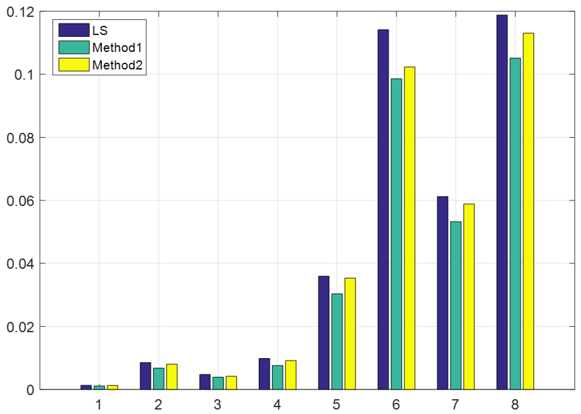
$J_e=\frac{\partial \Psi }{\partial e^T}$ and $J_{\xi }=\frac{\partial \Psi }{\partial {\xi }^T}$ are needed to obtain the GHM model results. First, we change the form of equation $\Psi$ to:

$$\Psi =(A+V_A)R^T+l_n^T\otimes t^T-Y-V_y=(R\otimes I_n)\times vec(A+V_A)+t\otimes l_n-vec(Y+V_y),$$

(20)

where e is linear in Equation (5), and $J_e$ is easily obtained as:

$$J_e=\left[\begin{array}{cc}\frac{\partial \Psi }{\partial vec{(V_A)}^T}& \frac{\partial \Psi }{\partial vec{(V_y)}^T}\end{array}\right]={\left[R\otimes I_n-I_3\otimes I_n\right]}_{3n\times 6n},$$

(21)

where $I_n$ is an identity matrix of dimension n. Then we need to calculate $J_{\xi }=\frac{\partial \psi }{\partial {\xi }^T}$.

Method 1: If we use parameterization method 1, then the Jacobian matrix is:

$$J_{\xi }={\left[\begin{array}{cc}\frac{\partial \Psi }{\partial \left[\begin{array}{ccc}{\varphi }_1& {\varphi }_2& {\varphi }_3\end{array}\right]}& \frac{\partial \Psi }{\partial \left[\begin{array}{ccc}{t}_1& t_2& t_3\end{array}\right]}\end{array}\right]}_{3n\times 6},$$

(22)

$\frac{\partial \psi }{\partial \left[\begin{array}{ccc}{t}_1& t_2& t_3\end{array}\right]}$ is easily obtained from Equation (20) as:

$$\frac{\partial \psi }{\partial \left[\begin{array}{ccc}{t}_1& t_2& t_3\end{array}\right]}=I_3\otimes l_n,$$

(23)

$\frac{\partial \psi }{\partial \left[\begin{array}{ccc}{\varphi }_1& {\varphi }_2& {\varphi }_3\end{array}\right]}$ can be simplified as follows:

$$\frac{\partial \psi }{\partial \left[\begin{array}{ccc}{\varphi }_1& {\varphi }_2& {\varphi }_3\end{array}\right]}={\left[\begin{array}{ccc}vec\left(\frac{\partial (A+V_A)R^T}{\partial {\varphi }_1}\right)& vec\left(\frac{\partial (A+V_A)R^T}{\partial {\varphi }_2}\right)& vec\left(\frac{\partial (A+V_A)R^T}{\partial {\varphi }_2}\right)\end{array}\right]}_{3n\times 3},$$

(24)

According to deductions from Appendix A, we know that:

$$\frac{\partial Rp}{\partial \left[\begin{array}{ccc}{\varphi }_1& {\varphi }_2& {\varphi }_3\end{array}\right]}=-{(Rp)}^{\wedge }.$$

(25)

We let $R(X_i+\Delta X_i)={\left[\begin{array}{ccc}{f}_i& g_i& h_i\end{array}\right]}^T$, so we can obtain the following equation:

$$\frac{\partial R(X_i+\Delta X_i)}{\partial \left[\begin{array}{ccc}{\varphi }_1& {\varphi }_2& {\varphi }_3\end{array}\right]}=\left[\begin{array}{ccc}\frac{\partial f_i}{\partial {\varphi }_1}& \frac{\partial f_i}{\partial {\varphi }_2}& \frac{\partial f_i}{\partial {\varphi }_3}\\ \frac{\partial g_i}{\partial {\varphi }_1}& \frac{\partial g_i}{\partial {\varphi }_2}& \frac{\partial g_i}{\partial {\varphi }_3}\\ \frac{\partial h_i}{\partial {\varphi }_1}& \frac{\partial h_i}{\partial {\varphi }_2}& \frac{\partial h_i}{\partial {\varphi }_3}\end{array}\right],$$

(26)

The elements in Equation (26) can be obtained from Equation (25). Thus, $\frac{\partial \psi }{\partial \left[\begin{array}{ccc}{\varphi }_1& {\varphi }_2& {\varphi }_3\end{array}\right]}$ is equal to:

$$\frac{\partial vec(A+V_A)R^T}{\partial {\varphi }_1}={\left[\begin{array}{ccc}\frac{\partial f_1}{\partial {\varphi }_1}& \frac{\partial g_1}{\partial {\varphi }_1}& \frac{\partial h_1}{\partial {\varphi }_1}\\ \frac{\partial f_2}{\partial {\varphi }_1}& \frac{\partial g_2}{\partial {\varphi }_1}& \frac{\partial h_2}{\partial {\varphi }_1}\\ \dots & \dots & \dots \\ \frac{\partial f_n}{\partial {\varphi }_1}& \frac{\partial g_n}{\partial {\varphi }_1}& \frac{\partial h_n}{\partial {\varphi }_1}\end{array}\right]}_{n\times 3},$$

(27)

$$\frac{\partial vec(A+V_A)R^T}{\partial {\varphi }_2}={\left[\begin{array}{ccc}\frac{\partial f_1}{\partial {\varphi }_2}& \frac{\partial g_1}{\partial {\varphi }_2}& \frac{\partial h_1}{\partial {\varphi }_2}\\ \frac{\partial f_2}{\partial {\varphi }_2}& \frac{\partial g_2}{\partial {\varphi }_2}& \frac{\partial h_2}{\partial {\varphi }_2}\\ \dots & \dots & \dots \\ \frac{\partial f_n}{\partial {\varphi }_2}& \frac{\partial g_n}{\partial {\varphi }_2}& \frac{\partial h_n}{\partial {\varphi }_2}\end{array}\right]}_{n\times 3},$$

(28)

$$\frac{\partial vec(A+V_A)R^T}{\partial {\varphi }_3}={\left[\begin{array}{ccc}\frac{\partial f_1}{\partial {\varphi }_3}& \frac{\partial g_1}{\partial {\varphi }_3}& \frac{\partial h_1}{\partial {\varphi }_3}\\ \frac{\partial f_2}{\partial {\varphi }_3}& \frac{\partial g_2}{\partial {\varphi }_3}& \frac{\partial h_2}{\partial {\varphi }_3}\\ \dots & \dots & \dots \\ \frac{\partial f_n}{\partial {\varphi }_3}& \frac{\partial g_n}{\partial {\varphi }_3}& \frac{\partial h_n}{\partial {\varphi }_3}\end{array}\right]}_{n\times 3},$$

(29)

The estimated parameters in method 1 are the Lie algebra of SO (3) and the translation vector. Thus, the update parameter is equal to ${[\begin{array}{cc}\Delta \varphi & \Delta t\end{array}]}^T$. The translation vector is in Euclidean space, so it is easy to update the new translation variable: $t_{k+1}=t_k+\Delta t$. $\Delta \varphi$ belongs to the Lie algebra of SO (3), and the updated formula is:

$${\varphi }_{k+1}=ln{(exp(\Delta {\varphi }^{\wedge })R_k)}^{\vee },$$

(30)

$R_k$ is the kth step rotation matrix. The operator “$\wedge$” is defined in Section 2.4. The “$ln{()}^{\vee }$” operator transforms the Lie group of SO (3) to the Lie algebra of SO (3). We do not provide specific expressions for “$ln{()}^{\vee }$” here; these can be found in [17]. In Appendix A, we deduce the Jacobian of Equation (25) using left multiplication so that update Formula (30) also uses left multiplication. Thus, the method 1 parameter update formula is:

$${\xi }_{k+1}={\xi }_k\oplus \delta \xi ={\left[\begin{array}{cc}{t}_k+\Delta t& ln{(exp(\Delta {\varphi }^{\wedge })R_k)}^{\vee }\end{array}\right]}^T,$$

(31)

Method 2: If we use parameterization method 2, the Jacobian matrix is:

$$J_{\xi }=\left[\begin{array}{cc}\frac{\partial \Psi }{\partial \left[\begin{array}{ccc}{\rho }_1& {\rho }_2& {\rho }_3\end{array}\right]}& \frac{\partial \Psi }{\partial \left[\begin{array}{ccc}{\varphi }_1& {\varphi }_2& {\varphi }_3\end{array}\right]}\end{array}\right].$$

(32)

From Appendix B, we know that:

$$\frac{\partial Tp}{\partial \xi }=\left[\begin{array}{cc}I& -{(Rp+t)}^{\wedge }\end{array}\right],$$

(33)

The left side of Equation (33) uses homogeneous coordinates, and the right side uses inhomogeneous coordinates. We transform homogeneous coordinate to inhomogeneous coordinates by default. We let $T(X_i+\Delta X_i)={\left[\begin{array}{ccc}{f}_i& g_i& h_i\end{array}\right]}^T$, so we can obtain the following equation:

$$\frac{\partial T(X_i+\Delta X_i)}{\partial \xi }=\left[\begin{array}{cccccc}\frac{\partial f_i}{\partial {\rho }_1}& \frac{\partial f_i}{\partial {\rho }_2}& \frac{\partial f_i}{\partial {\rho }_3}& \frac{\partial f_i}{\partial {\varphi }_1}& \frac{\partial f_i}{\partial {\varphi }_2}& \frac{\partial f_i}{\partial {\varphi }_3}\\ \frac{\partial g_i}{\partial {\rho }_1}& \frac{\partial g_i}{\partial {\rho }_2}& \frac{\partial g_i}{\partial {\rho }_3}& \frac{\partial g_i}{\partial {\varphi }_1}& \frac{\partial g_i}{\partial {\varphi }_2}& \frac{\partial g_i}{\partial {\varphi }_3}\\ \frac{\partial h_i}{\partial {\rho }_1}& \frac{\partial h_i}{\partial {\rho }_2}& \frac{\partial h_i}{\partial {\rho }_3}& \frac{\partial h_i}{\partial {\varphi }_1}& \frac{\partial h_i}{\partial {\varphi }_2}& \frac{\partial h_i}{\partial {\varphi }_3}\end{array}\right],$$

(34)

The elements in Equation (34) can be obtained by Equation (35). Thus, we have:

$$J_{\xi }={\left[\begin{array}{cccccc}\frac{\partial f_1}{\partial {\rho }_1}& \frac{\partial f_1}{\partial {\rho }_2}& \frac{\partial f_1}{\partial {\rho }_3}& \frac{\partial f_1}{\partial {\varphi }_1}& \frac{\partial f_1}{\partial {\varphi }_2}& \frac{\partial f_1}{\partial {\varphi }_3}\\ \dots & \dots & \dots & \dots & \dots & \dots \\ \frac{\partial f_n}{\partial {\rho }_1}& \frac{\partial f_n}{\partial {\rho }_2}& \frac{\partial f_n}{\partial {\rho }_3}& \frac{\partial f_n}{\partial {\varphi }_1}& \frac{\partial f_n}{\partial {\varphi }_2}& \frac{\partial f_n}{\partial {\varphi }_3}\\ \frac{\partial g_1}{\partial {\rho }_1}& \frac{\partial g_1}{\partial {\rho }_2}& \frac{\partial g_1}{\partial {\rho }_3}& \frac{\partial g_1}{\partial {\varphi }_1}& \frac{\partial g_1}{\partial {\varphi }_2}& \frac{\partial g_1}{\partial {\varphi }_3}\\ \dots & \dots & \dots & \dots & \dots & \dots \\ \frac{\partial g_n}{\partial {\rho }_1}& \frac{\partial g_n}{\partial {\rho }_2}& \frac{\partial g_n}{\partial {\rho }_3}& \frac{\partial g_n}{\partial {\varphi }_1}& \frac{\partial g_n}{\partial {\varphi }_2}& \frac{\partial g_n}{\partial {\varphi }_3}\\ \frac{\partial h_1}{\partial {\rho }_1}& \frac{\partial h_1}{\partial {\rho }_2}& \frac{\partial h_1}{\partial {\rho }_3}& \frac{\partial h_1}{\partial {\varphi }_1}& \frac{\partial h_1}{\partial {\varphi }_2}& \frac{\partial h_1}{\partial {\varphi }_3}\\ \dots & \dots & \dots & \dots & \dots & \dots \\ \frac{\partial h_n}{\partial {\rho }_1}& \frac{\partial h_n}{\partial {\rho }_2}& \frac{\partial h_n}{\partial {\rho }_3}& \frac{\partial h_n}{\partial {\varphi }_1}& \frac{\partial h_n}{\partial {\varphi }_2}& \frac{\partial h_n}{\partial {\varphi }_3}\end{array}\right]}_{3n\times 6},$$

(35)

The estimated parameters in method 2 are the Lie algebra of SE (3). The update parameter is equal to $\Delta \xi$, which belongs to the Lie algebra of SE (3), and the updated formula is:

$${\xi }_{k+1}=ln{(exp(\Delta {\xi }^{\wedge })T_k)}^{\vee },$$

(36)

where $T_k$ is the kth step rigid transformation matrix. The Operator “$\wedge$” is defined in Section 2.4. The operator “$ln{()}^{\vee }$” transforms the Lie group of SE (3) to the Lie algebra of SE (3). We provide no specific expressions for “$ln{()}^{\vee }$.” These can be found in [17]. In Appendix B, we deduce the Jacobian of Equation (33) using left multiplication, so that update Equation (36) also uses left multiplication. Thus, the method 2 parameter updated formula is:

$${\xi }_{k+1}={\xi }_k\oplus \delta \xi =ln{(exp(\Delta {\xi }^{\wedge })T_k)}^{\vee },$$

(37)

3. Experiments

In this section, we use the dataset from [9]. This numerical example is from an actual experiment of fitting two surfaces that are surveyed in two different reference systems. Four control points are chosen in two different coordinate systems. We assume that we have a known scale equal to 2.1, and we multiply the source coordinate by 2.1. Data from [9] are shown in

Table 2. A numerical example.

Point No.	Source x	Source y	Source z	Target x’	Target y’	Target z’
1	63	84	21	290	150	15
2	210	84	21	420	80	2
3	210	273	21	540	200	20
4	63	273	21	390	300	5

. We compare the LS- and TLS-ICP algorithms using simulated data and demonstrate that the TLS-ICP algorithm is more accurate. Then we use real measurement data from Table 2 and demonstrate that the TLS algorithm has a smaller residual error than the LS method.

First, we compare results from TLS and LS using simulated data. A true translation vector is set to (190, 110, −15), and a rotation matrix is constructed by the Euler angle. The true rotation angles around the z-, y-, and x-axes are set to 45 degrees, 90 degrees, and 60 degrees, respectively. Then, we generate controlled points in target coordinates according to the true rotation matrix, true translation, and controlled points in the source coordinate. We add noise in the source and target coordinates according to two distributions: normal and uniform. We classify noise into eight classes, as shown in

Table 3. Noise type and variance for each class.

Noise Number	Noise Type	x	y	z	Noise Number	Noise Type	x	y	z
1	Normal	0.1	0.1	0.1	5	Uniform	5	5	5
2	Normal	0.1	0.5	1	6	Uniform	5	10	20
3	Normal	0.1	0.5	0.5	7	Uniform	5	10	10
4	Normal	0.1	1	1	8	Uniform	5	20	20

. The normal distribution is a Gaussian distribution with zero mean and a covariance. We use the uniform distribution to generate samples in some range, and every sample is generated by equal chance. In the first row of Table 3, 0.1 is the variance of the Gaussian distribution, and a noise number of 5 means that the uniform distribution generates samples ranging from −5 to 5.

The rotation error is:

$$Erro{r}_R=acos(max(min(0.5\ast \left(\Delta R(0,0\right)+\Delta R(1,1)+\Delta R(2,2)),1),-1),$$

(38)

where $\Delta R=R_{true}^T{R}_{TLS}$, $R_{TLS}$ is the rotation matrix from the TLS algorithm, and $R_{true}$ is the true rotation matrix. The error measure in Equation (38) describes how close $\Delta R$ is to the identity matrix. If $\Delta R$ is closer to the identity matrix, then our algorithm is more accurate. The translation error is evaluated as $Erro{r}_t=\Vert t_{true}-t_{TLS}\Vert$, where $t_{TLS}$ is the translation from the TLS algorithm, and $t_{true}$ is the true translation.

If noise is generated by a normal distribution, then the information matrix p is set to the inverse of the variance. If noise is generated by a uniform distribution, then the information matrix p is set to the identity matrix. Figure 1 and Figure 2 show the rotation error and translation error, respectively, of least-squares, method 1, and method 2. We see from these figures that larger variances between the x-, y-, and z-axes lead to a larger error of the least-squares method. This is because the rotation matrix is obtained by the Procrustes approach [9], which assumes that noise in the x-, y-, and z-axes is equal. In this situation, the LS algorithm is nearly as accurate as the TLS algorithm, and we can see this result in the first column of Figure 1 and Figure 2. However, the TLS algorithm performs much better than the LS algorithm when variances between the x-, y-, and z-axes become large, as shown in the fourth column and the eighth column in Figure 1 and Figure 2. Method 1 is more accurate than method 2 in estimating the rotation matrix, but method 2 is more accurate than method 1 in estimating the translation vector. This phenomenon is caused by different parameterization approaches in these two methods. The parameterization of method 2 uses the Lie algebra of SE (3), which is a six-dimensional vector. The first three elements in this vector describe the translation and rotation matrices. The last three elements only describe the rotation matrix. The first three elements are optimized during the TLS iterative process, and then we recover the translation vector using the last three elements in the Lie algebra vector. The benefit of this is that the Jacobian matrix conditional number is not so large, which means that the estimated parameters equally decide the direction of optimization. In Method 1, the Jacobian matrix of $\varphi$ is $-{(Rp)}^{\wedge }$, and the Jacobian matrix of t is always the identity matrix. If p is very large, then the Jacobian matrix of $\varphi$ mainly decides the direction of optimization, so that method 1 has a smaller rotation error than method 2.

Here, we directly use data from [12], which is an actual experiment of fitting two surfaces surveyed in two reference systems. Data are shown in Table 2, and the result is shown in

Table 4. The comparision between Lie algebra TLS, Euler Angle TLS and common LS algorithm.

Estimated Parameter	Euler Method	Estimated Parameter	Method 1	LS	Estimated Parameter	Method 2	LS
Z-axis angle (rad)	2.516	${\varphi }_1$	0.0207793	0.02066	${\xi }_1$	151.836	151.834
Y-axis angle (rad)	−3.137	${\varphi }_2$	−0.011339	−0.0112	${\xi }_2$	175.062	175.066
X-axis angle	−3.119	${\varphi }_3$	−0.625356	−0.6254	${\xi }_3$	−17.5989	−17.6049
$t_1$	195.23	$t_1$	195.231	195.23	${\xi }_4$	0.02065	0.02066
$t_2$	118.064	$t_2$	118.064	118.067	${\xi }_5$	0.0112623	0.01128
$t_3$	−15.138	$t_3$	−15.1442	−15.143	${\xi }_6$	−0.62536	−0.6253
SSE	1.14	SSE	0.0564	68.577	SSE	0.005056	68.577

. We give results of LS, TLS based on Euler angle, method 1, and method 2. Our two methods have much smaller sums of residual errors than the LS method. This is mainly because the TLS algorithm considers noise from the source and target coordinate systems. Further discussion of errors and the model are beyond the scope of this paper; refer to Grafarend [18]. Compared to the Euler angle method, our method has smaller SSE after optimization, which proves that Lie algebra is more suitable for the TLS-ICP algorithm. We should note that our method also can be used in similar transformation estimation. The difference is that the Jacobian of scale s is needed for additional calculations.

TLS-ICP algorithm often uses 4–8 points to calculate transformation between two coordinates in geological mapping. Thus, in previous experiments, datasets from [9] are used to evaluate accuracy. However, in the field of three-dimensional reconstruction, ICP algorithm also can be used to calculate robot pose. Thus, the cost time of ICP is very important. In our experiment, all of codes run on a laptop with 2.7 GHz quad cores in Ubuntu. We use 100 points, 500 points, and 1000 points, which are copied from [9], to evaluate the cost time of every step in our algorithm. The cost time of every iterative step is 0.2 ms using four points. The cost time of every iterative step is 380 ms using 100 points. The cost time of every iterative step is 46 s using 500 points. The cost time of every iterative step is 369 s using 1000 points. In our experiment, the process of our algorithm converges to final result after three or four steps.

4. Conclusions

In this paper, we present two total least-squares ICP algorithms based on Lie algebra using a GHM framework. These methods can estimate a rigid transformation matrix from adjusted source coordinates and adjusted target coordinates. Our methods perform better than the common least-squares ICP algorithm because they consider random noise from the source coordinate, which results in a smaller sum of squared errors. The most important contribution of this paper is that our methods are more robust than [12,19], which utilize the Euler angle to describe the rotation matrix. The nonlinearity in the cost function due to the rotation matrix results in there being no analytical solution to this problem. Thus, an iterative optimization algorithm is employed to solve the GHM model. The Euler angle is unsuitable for interpolation because of the gimbal lock problem. We replace the Euler angle with Lie algebra to execute the TLS optimization algorithm and give deduction of our method in detail.

References

1. Rusinkiewicz, S. Efficient variants of the ICP algorithm. Proc. 3DIM 2001, 1, 145–152. [Google Scholar]
2. Mur-Artal, R.; Montiel, J.M.M.; Tardós, J.D. Orb-slam: A versatile and accurate monocular slam system. IEEE Trans. Robot. 2015, 31, 1147–1163. [Google Scholar] [CrossRef] [Green Version]
3. Kreiberg, D.; Söderström, T.; Yang-Wallentin, F. Errors-in-variables system identification using structural equation modeling. Automatica 2016, 66, 218–230. [Google Scholar] [CrossRef] [Green Version]
4. Horn, B.K.P. Closed-form solution of absolute orientation using unit quaternions. Repr. J. Opt. Soc. Am. A 1987, 4, 629–642. [Google Scholar] [CrossRef]
5. Kummerle, R.; Grisetti, G.; Strasdat, H.; Konolige, K.; Burgard, W. G2o: A general framework for graph optimization. In Proceedings of the 2011 IEEE International Conference on Robotics and Automation, Shanghai, China, 9–13 May 2011. [Google Scholar]
6. Golub, G.H.; Van Loan, C.F. An Analysis of the Total Least Squares Problem. SIAM J. Numer. Anal. 1980, 17, 883–893. [Google Scholar] [CrossRef]
7. Shen, Y.; Li, B.; Chen, Y. An iterative solution of weighted total least-squares adjustment. J. Geod. 2011, 85, 229–238. [Google Scholar] [CrossRef]
8. Mahboub, V. On weighted total least-squares for geodetic transformations. J. Geod. 2012, 86, 359–367. [Google Scholar] [CrossRef]
9. Felus, Y.A.; Burtch, R.C. On symmetrical three-dimensional datum conversion. GPS Solut. 2009, 13, 65–74. [Google Scholar] [CrossRef]
10. Estépar, R.S.J.; Brun, A.; Westin, C.F. Robust Generalized Total Least Squares Iterative Closest Point Registration. Medical Image Computing and Computer-Assisted Intervention—MICCAI 2004. MICCAI 2004. In Lecture Notes in Computer Science; Barillot, C., Haynor, D.R., Hellier, P., Eds.; Springer: Berlin/Heidelberg, Germany, 2004; Volume 3216. [Google Scholar]
11. Ohta, N.; Kanatani, K. Optimal estimation of three-dimensional rotation and reliability evaluation. IEICE Trans. Inf. Syst. 1998, 81, 1247–1252. [Google Scholar]
12. Fang, X. A total least squares solution for geodetic datum transformations. Acta Geod. Geophys. 2014, 49, 189–207. [Google Scholar] [CrossRef]
13. Chang, G. On least-squares solution to 3D similarity transformation problem under Gauss–Helmert model. J. Geod. 2015, 89, 573–576. [Google Scholar] [CrossRef]
14. Fang, X. Weighted total least-squares with constraints: A universal formula for geodetic symmetrical transformations. J. Geod. 2015, 89, 459–469. [Google Scholar] [CrossRef]
15. Wang, B.; Li, J.; Liu, C.; Yu, J. Generalized total least squares prediction algorithm for universal 3D similarity transformation. Adv. Space Res. 2017, 59, 815–823. [Google Scholar] [CrossRef]
16. Koch, K. Robust estimations for the nonlinear Gauss Helmert model by the expectation maximization algorithm. J. Geod. 2014, 88, 263–271. [Google Scholar] [CrossRef]
17. Barfoot, T.D. State Estimation for Robotics; Cambridge University Press: Cambridge, UK, 2017. [Google Scholar]
18. Teunissen, P. Applications of linear and nonlinear models: Fixed effects, random effects, and total least squares. Surveyor 2012, 58, 339–340. [Google Scholar] [CrossRef]
19. Schaffrin, B.; Felus, Y.A. On the multivariate total least-squares approach to empirical coordinate transformations. Three algorithms. J. Geod. 2008, 82, 373–383. [Google Scholar] [CrossRef]
Figure 1. The rotation error is compared between least-squares and our proposed methods. The blue, green, and yellow bars are the rotation errors of least-squares, method 1, and method 2, respectively. The x-axis of this figure is a different noise class shown in Table 3.
Applsci 09 05352 g001
Figure 2. The translation error is compared between least-squares method and our proposed methods. The blue, green, and yellow bars are the translation errors of least-squares, method 1, and method 2, respectively. The x-axis of this figure is a different noise class shown in Table 3.
Applsci 09 05352 g002