Geometric and Radiometric Consistency of Parrot Sequoia Multispectral Imagery for Precision Agriculture Applications


Abstract
1. Introduction
1.1. Key Topics
1.2. Background
1.3. Motivation
2. Methods
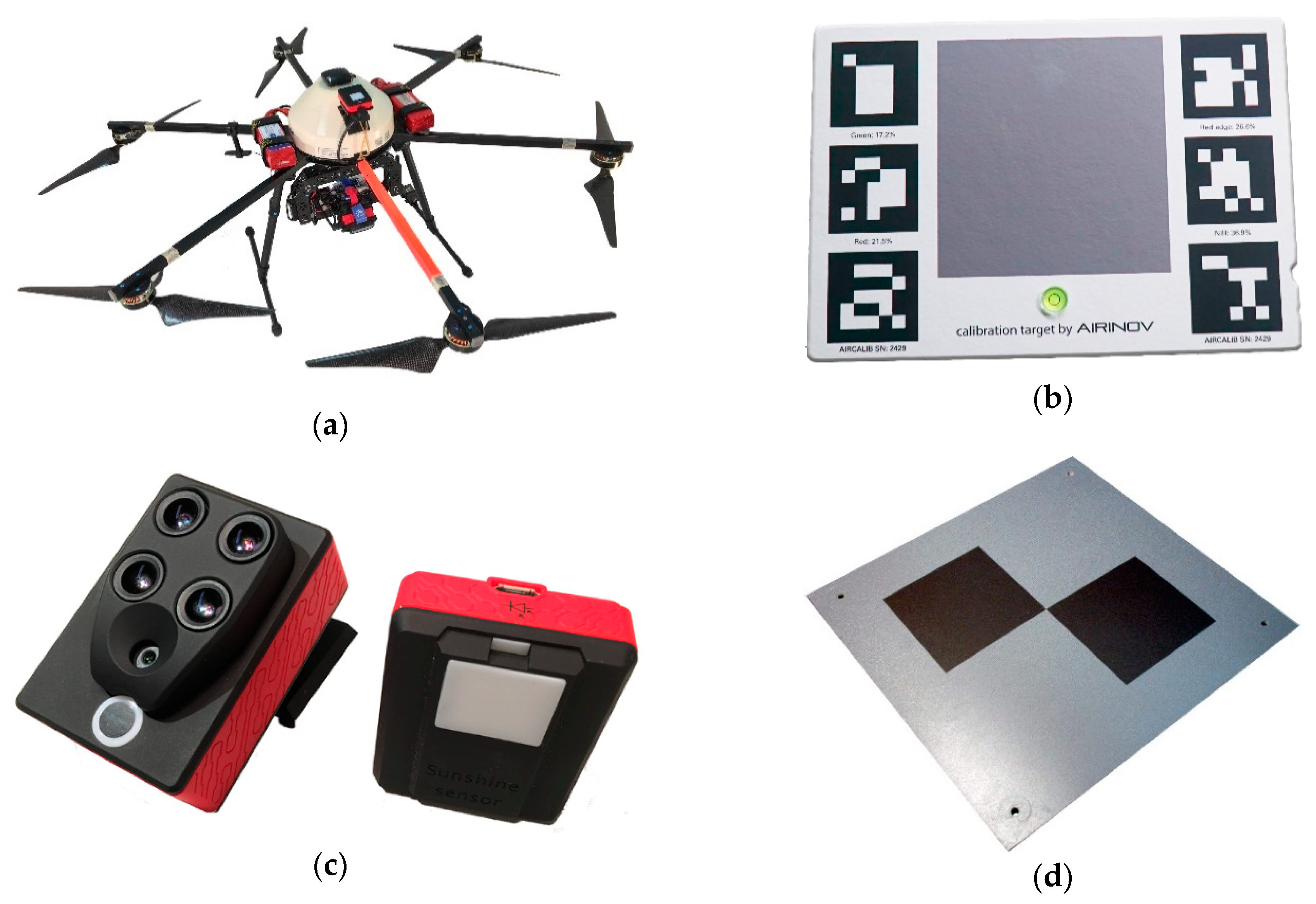
2.1. The Equipment
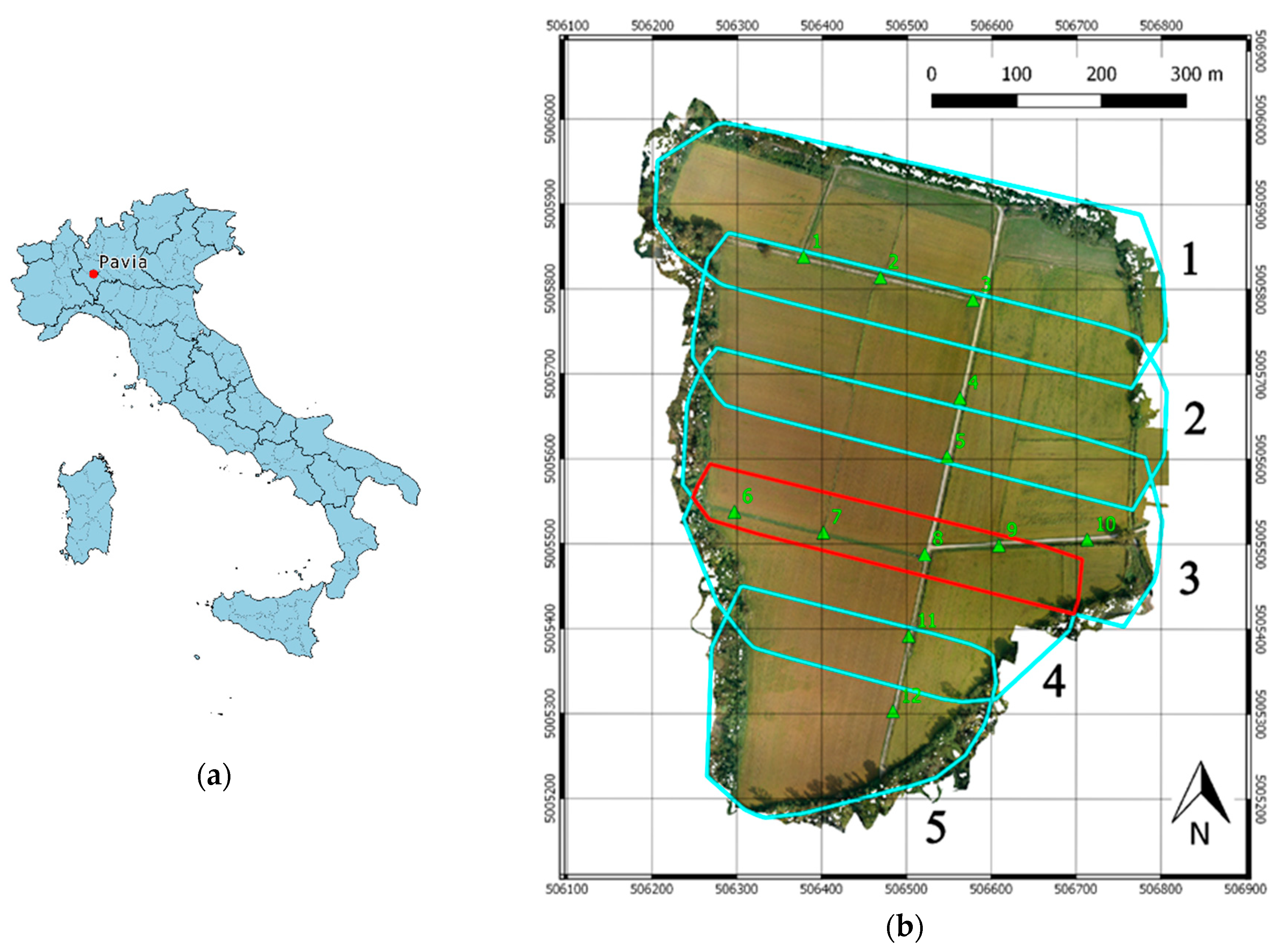
2.2. The Block Structure
2.3. The Photogrammetric Processing
- Direct georeferencing (DG) scenario: no GCPs were inserted in the BBA and each sub-block was processed by direct photogrammetry using positions from the Sequoia integrated GPS receiver. This scenario was used only in geometric assessment.
- Independent georeferentiation/independent radiometric processing (Ig/Ir) scenario: the two blocks were independently processed in terms of geometry and radiometry. This scenario was used both in geometric and radiometric assessment.
- Independent georeferentiation/joint radiometric processing (Ig/Jr) scenario: this scenario is a variation of the previous one, in which orientation parameters were computed for each block independently, as in the second scenario, but the two flights were then merged for dense point cloud and reflectance maps generation. This scenario coincides with the so-called “merge option” in Pix4Dmapper software, and it is the recommended procedure for processing photogrammetric blocks with a large number of images and an overlapping area. It should ensure that radiometric differences caused by a misalignment in the dense point clouds are avoided. Scenario Ig/Jr was used only in radiometric assessment.
- Joint georeferentiation/independent radiometric processing (Jg/Ir) scenario: the two blocks were jointly orientated, and the obtained exterior orientation parameters were then transferred to a single-block project for generation of dense point clouds and reflectance maps. In this scenario, possible radiometric inconsistencies due to separate computation of interior and exterior orientation parameters are eliminated. This scenario was used in both geometric and radiometric assessment.
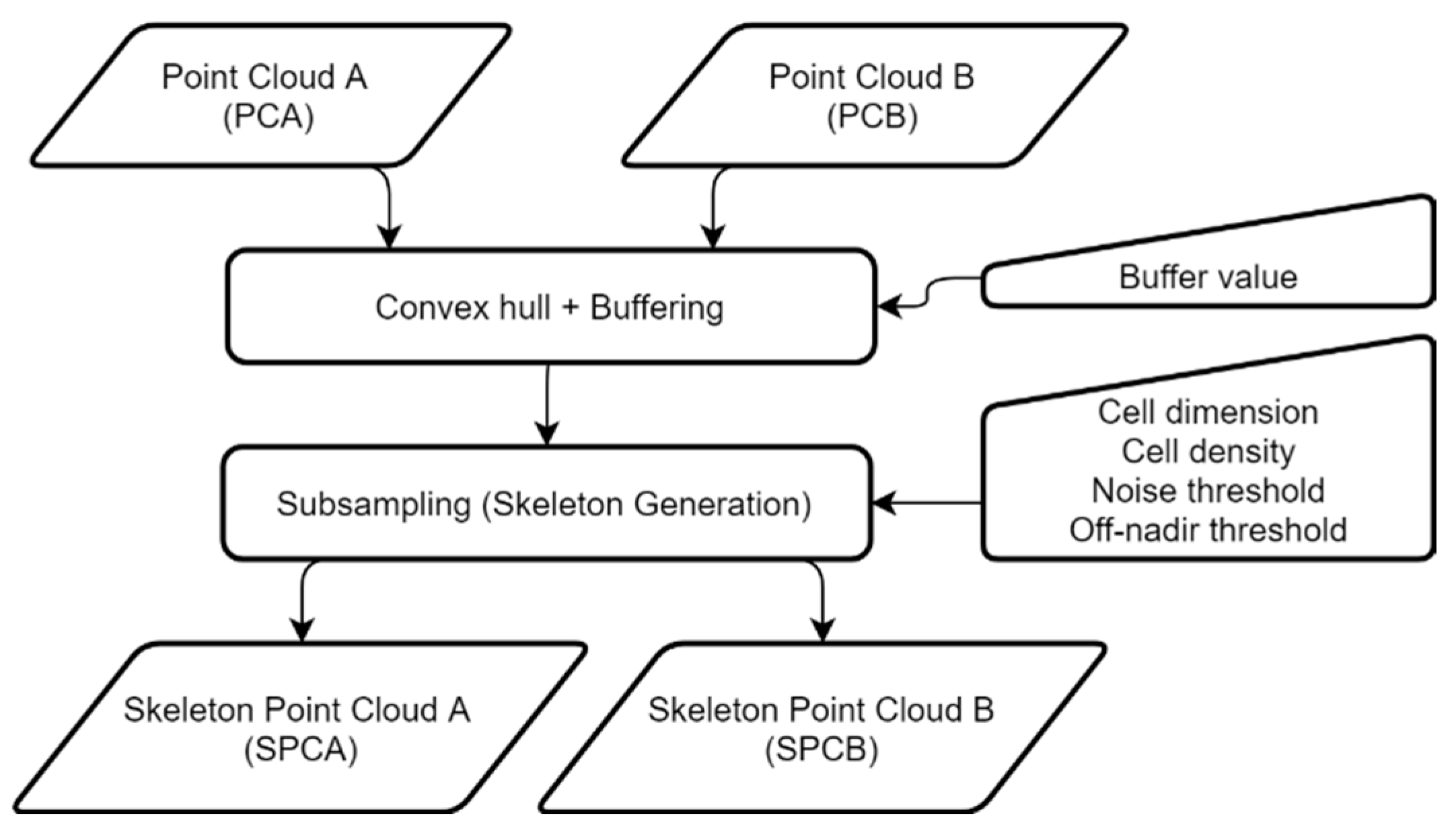
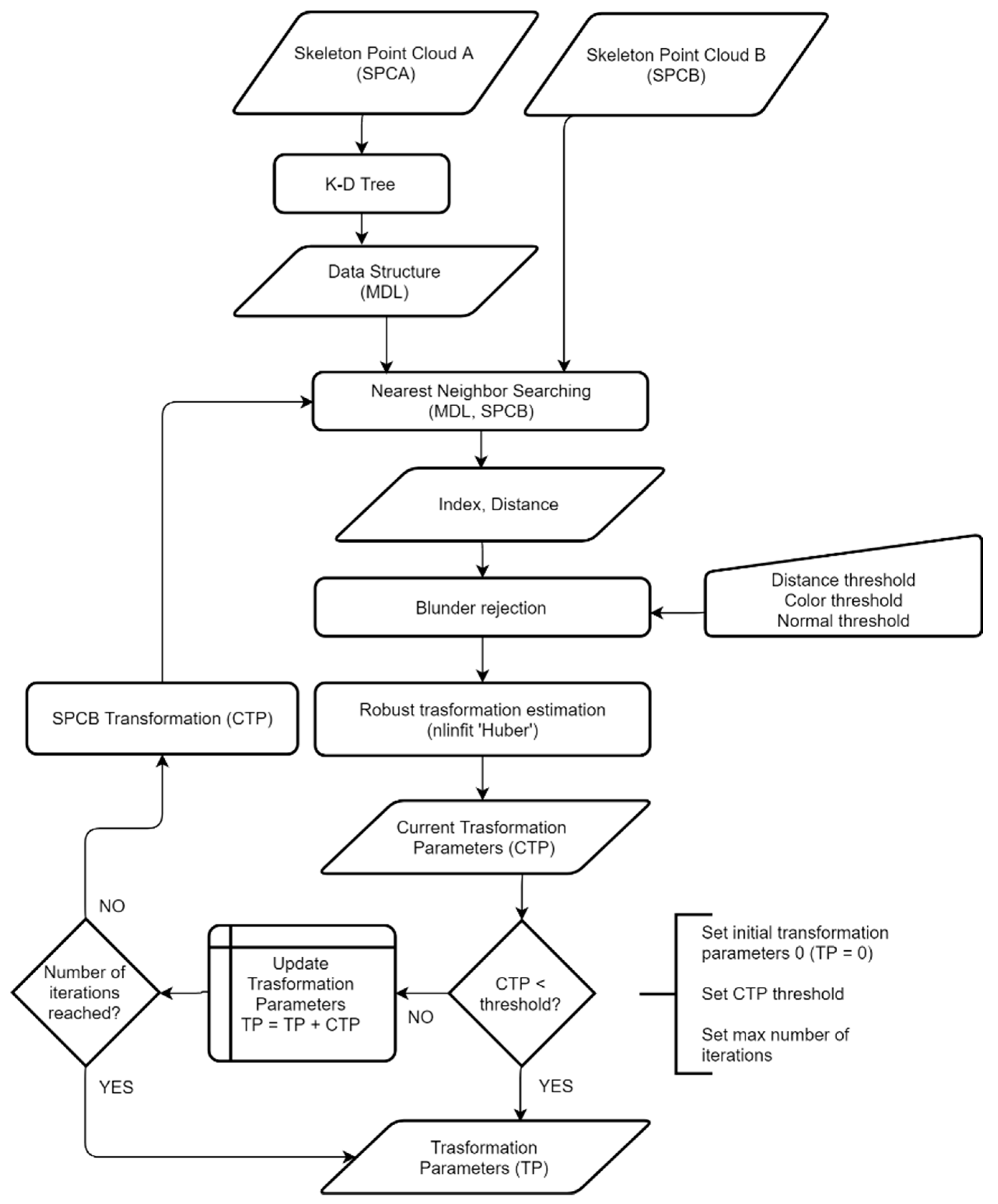
2.4. Geometric Consistency Assessment
- has in its input the running SPCB (produced by the previous iteration; in the first iteration, this is SPCB itself), the SPCA (remaining unaltered for all the process), and the running 3D rigid transformation determined so far;
- couples each point of the running SPCB with the closest point belonging to SPCA;
- performs outlier rejection based on the points’ distances, the angle between the surface normals at the two points considered, and the norm of the difference between their RGB vectors;
- determines the parameters of a refinement of the 3D rigid transformation aligning running SPCB and SPCA, by solving a non-linear least squares (NLLS) problem defined by Equation (1); in plain words, the NLLS solver evaluates the distance between each B-point (belonging to running SPCB) and the plane passing through the paired A-point (belonging to SPCA) and the normal to SPCA; it determines the unknowns in order to minimize the sum of all the distances;
- applies the determined 3D transformation to the running SPCB;
- composes the newly determined transformation with that received in the input;
- returns the updated running SPCB and coordinate transformation.
2.5. Radiometric Consistency Assessment
3. Results
3.1. Geometric Consistency
3.1.1. Reliability of the ICP-Derived Transformations
3.1.2. Assessment of the Distance between Overlapping Blocks
3.2. Radiometric Consistency
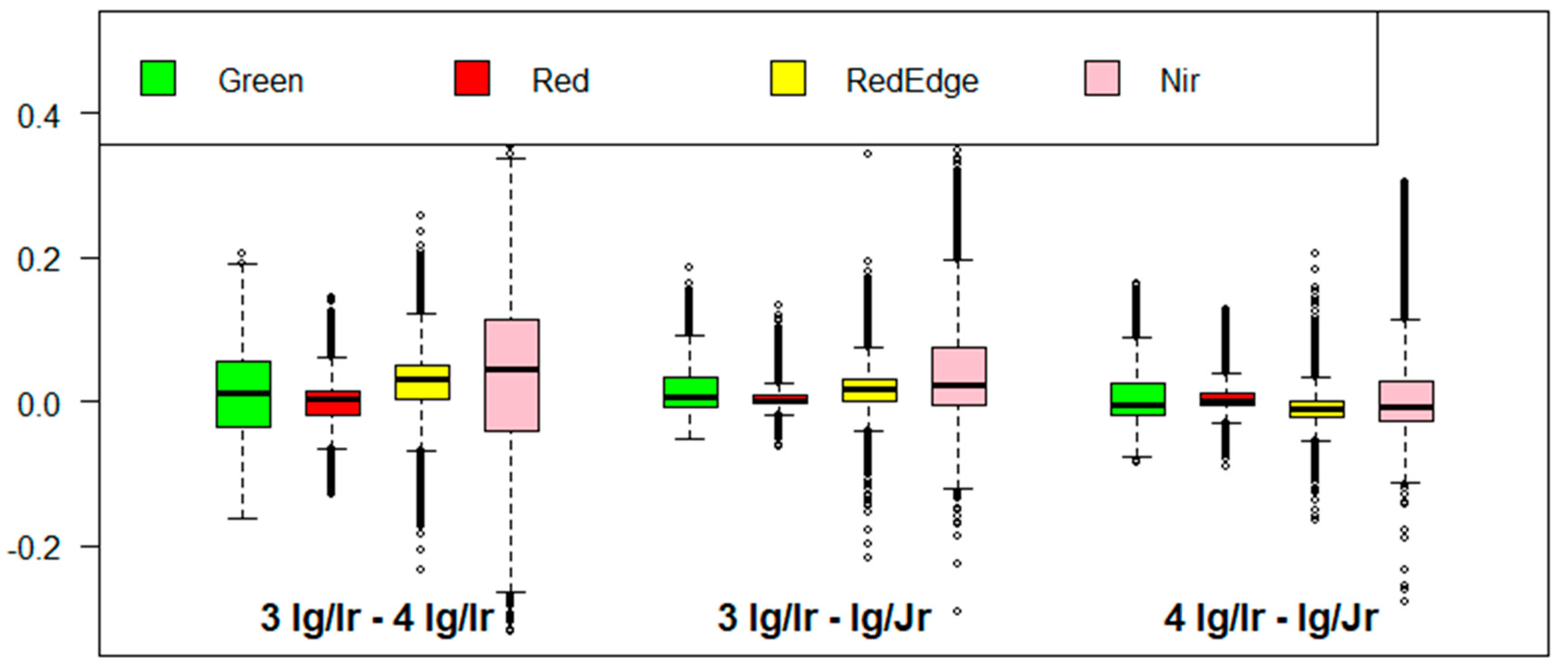
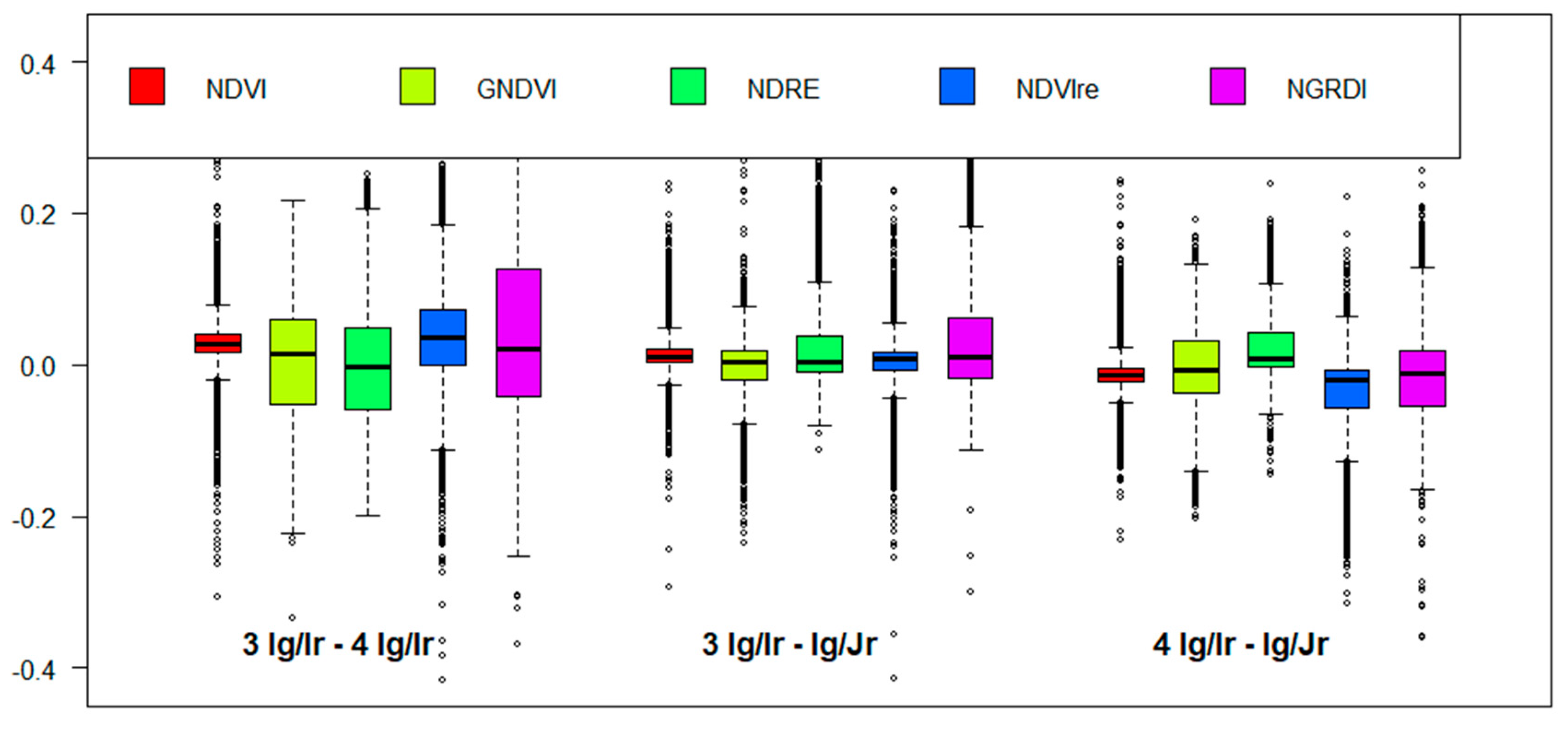
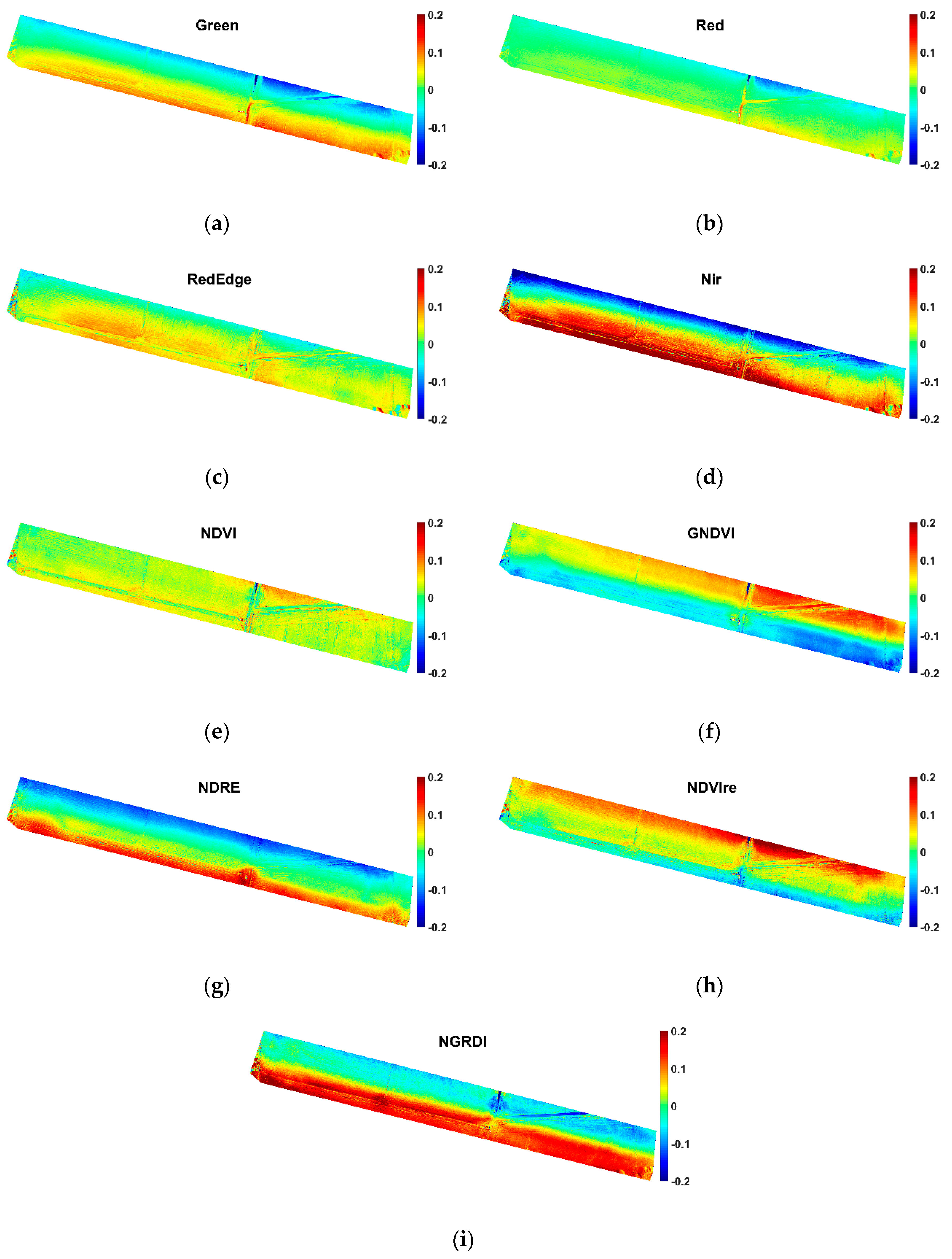
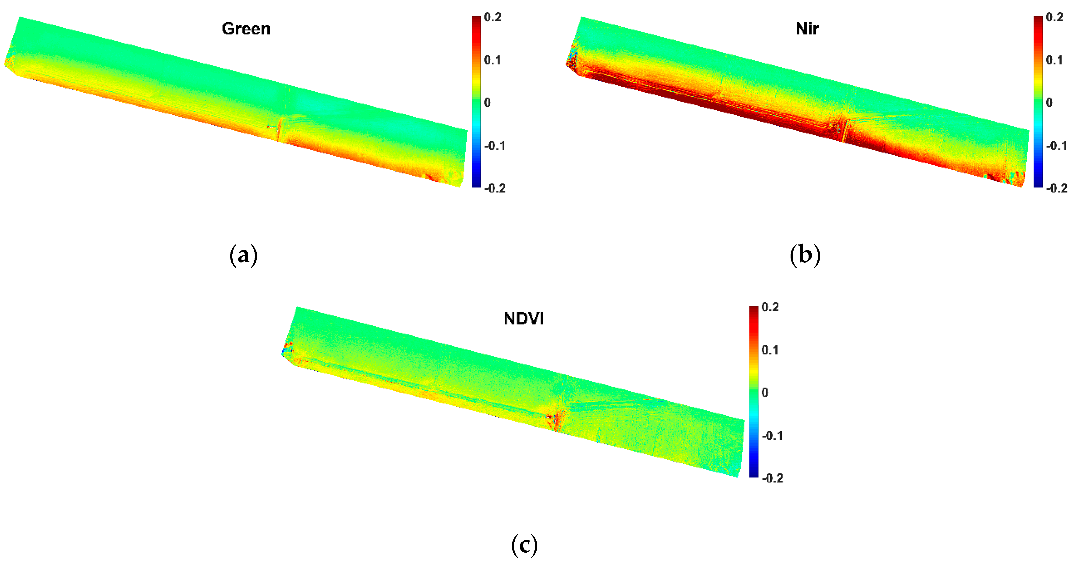
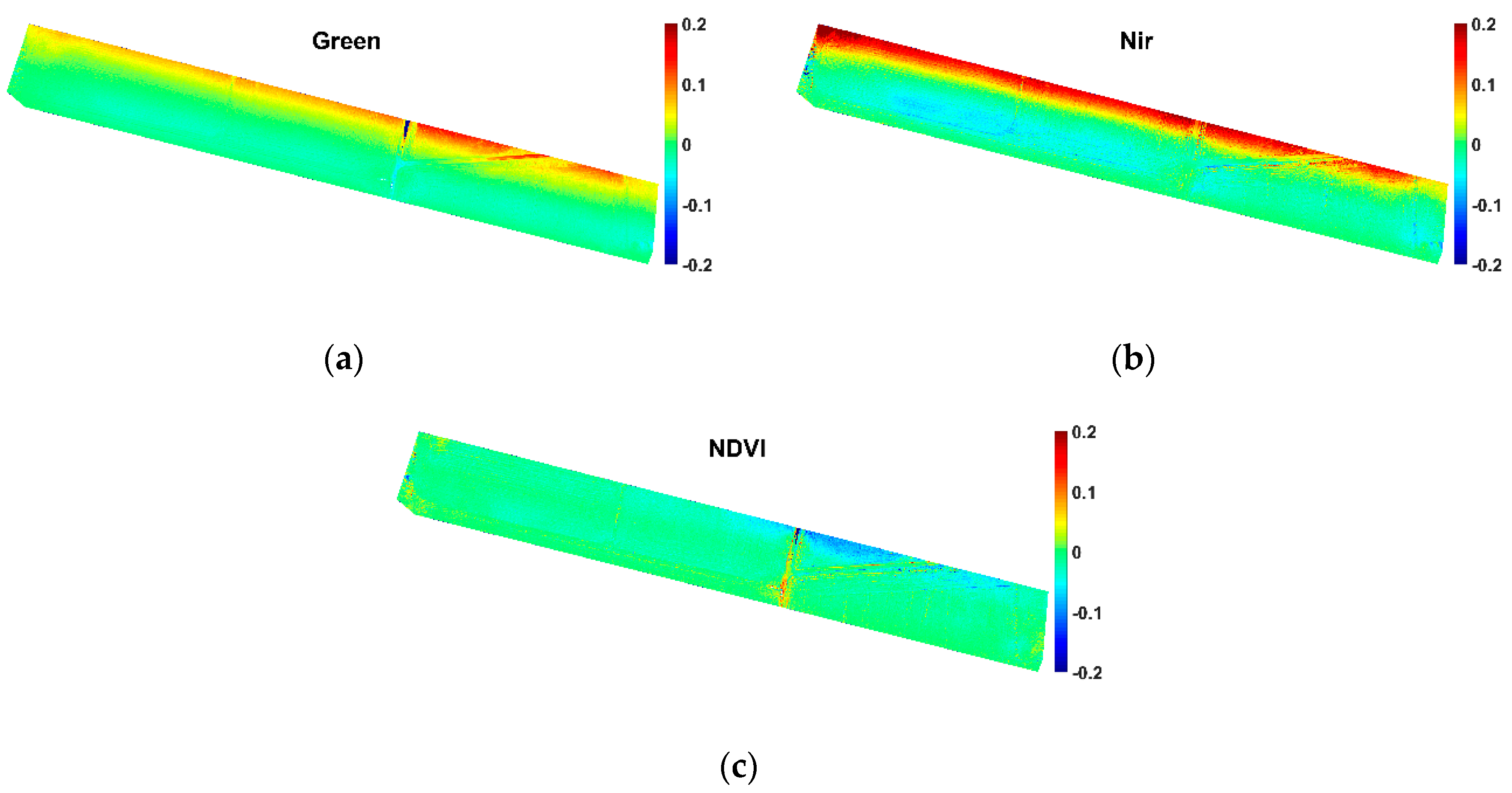
3.2.1. Assessment of the Radiometric Differences between Overlapping Blocks
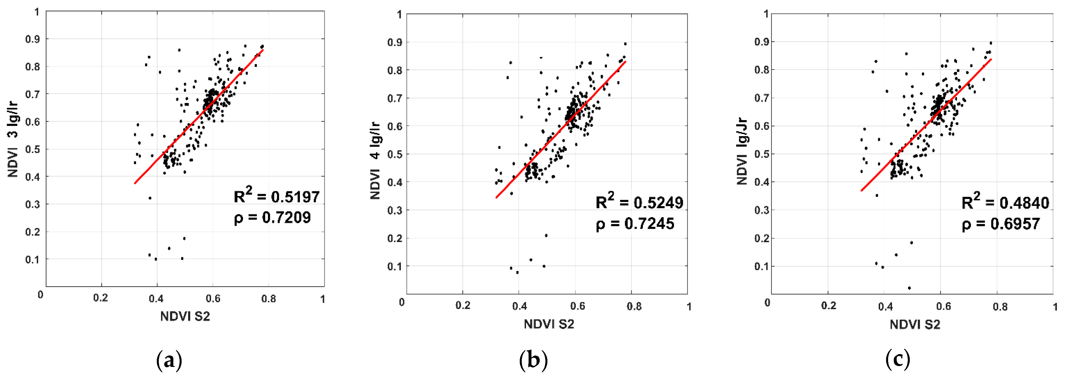
3.2.2. Comparison with Sentinel-2 Imagery
4. Discussion
4.1. Geometric Consistency
4.2. Radiometric Consistency
5. Conclusions
Supplementary Materials
Author Contributions
Acknowledgments
Conflicts of Interest
References
- Candiago, S.; Remondino, F.; De Giglio, M.; Dubbini, M.; Gattelli, M. Evaluating multispectral images and vegetation indices for precision farming applications from UAV images. Remote Sens. 2015, 7, 4026–4047. [Google Scholar] [CrossRef]
- Schieffer, J.; Dillon, C. The economic and environmental impacts of precision agriculture and interactions with agro-environmental policy. Precis. Agric. 2015, 16, 46–61. [Google Scholar] [CrossRef]
- Turner, D.; Lucieer, A.; Watson, C. An automated technique for generating georectified mosaics from ultra-high resolution unmanned aerial vehicle (UAV) imagery, based on structure from motion (SfM) point clouds. Remote Sens. 2012, 4, 1392–1410. [Google Scholar] [CrossRef]
- Parrot. Available online: https://community.parrot.com/t5/Sequoia/bd-p/Sequoia (accessed on 13 June 2019).
- Chiang, K.W.; Tsai, M.L.; Chu, C.H. The development of an UAV borne direct georeferenced photogrammetric platform for ground control point free applications. Sensors 2012, 12, 9161–9180. [Google Scholar] [CrossRef]
- Lussem, U.; Bareth, G.; Bolten, A.; Schellberg, J. Feasibility study of directly georeferenced images from low-cost unmanned aerial vehicles for monitoring sward height in a long-term experiment on grassland. Grassl. Sci. Eur. 2017, 22, 354–356. [Google Scholar]
- Tahar, K.N. An evaluation on different number of ground control points in unmanned aerial vehicle photogrammetric block. Int. Arch. Photogramm. Remote Sens. Spat. Inf. Sci. 2013, 40, 93–98. [Google Scholar] [CrossRef]
- James, M.R.; Robson, S.; d’Oleire-Oltmanns, S.; Niethammer, U. Optimising UAV topographic surveys processed with structure-from-motion: Ground control quality, quantity and bundle adjustment. Geomorphology 2017, 280, 51–66. [Google Scholar] [CrossRef]
- Mesas-Carrascosa, F.J.; Torres-Sánchez, J.; Clavero-Rumbao, I.; García-Ferrer, A.; Peña, J.M.; Borra-Serrano, I.; López-Granados, F. Assessing optimal flight parameters for generating accurate multispectral orthomosaicks by UAV to support site-specific crop management. Remote Sens. 2015, 7, 12793–12814. [Google Scholar] [CrossRef]
- Assmann, J.J.; Kerby, J.T.; Cunliffe, A.M.; Myers-Smith, I.H. Vegetation monitoring using multispectral sensors—best practices and lessons learned from high latitudes. J. Unmanned Veh. Syst. 2018, 7, 54–75. [Google Scholar] [CrossRef]
- Fernández-Guisuraga, J.; Sanz-Ablanedo, E.; Suárez-Seoane, S.; Calvo, L. Using unmanned aerial vehicles in postfire vegetation survey campaigns through large and heterogeneous areas: Opportunities and challenges. Sensors 2018, 18, 586. [Google Scholar] [CrossRef]
- Caroti, G.; Martínez-Espejo Zaragoza, I.; Piemonte, A. Accuracy assessment in structure from motion 3D reconstruction from UAV-born images: The influence of the data processing methods. Int. Arch. Photogramm. Remote Sens. Spat. Inf. Sci. 2015, 40. [Google Scholar] [CrossRef]
- Benassi, F.; Dall’Asta, E.; Diotri, F.; Forlani, G.; Morra di Cella, U.; Roncella, R.; Santise, M. Testing accuracy and repeatability of UAV blocks oriented with GNSS-supported aerial triangulation. Remote Sens. 2017, 9, 172. [Google Scholar] [CrossRef]
- Martínez-Carricondo, P.; Agüera-Vega, F.; Carvajal-Ramírez, F.; Mesas-Carrascosa, F.J.; García-Ferrer, A.; Pérez-Porras, F.J. Assessment of UAV-photogrammetric mapping accuracy based on variation of ground control points. Int. J. Appl. Earth Obs. 2018, 72, 1–10. [Google Scholar] [CrossRef]
- Harwin, S.; Lucieer, A. Assessing the accuracy of georeferenced point clouds produced via multi-view stereopsis from unmanned aerial vehicle (UAV) imagery. Remote Sens. 2012, 4, 1573–1599. [Google Scholar] [CrossRef]
- Casella, V.; Franzini, M. Modelling steep surface by various configurations of nadir and oblique photogrammetry. ISPRS Ann. Photogramm. Remote Sens. Spat. Inf. Sci. 2016, 3. [Google Scholar] [CrossRef]
- Jaud, M.; Passot, S.; Le Bivic, R.; Delacourt, C.; Grandjean, P.; Le Dantec, N. Assessing the accuracy of high-resolution digital surface models computed by PhotoScan® and MicMac® in sub-optimal survey conditions. Remote Sens. 2016, 8, 465. [Google Scholar] [CrossRef]
- Fritz, A.; Kattenborn, T.; Koch, B. UAV-based photogrammetric point clouds—Tree stem mapping in open stands in comparison to terrestrial laser scanner point clouds. Int. Arch. Photogramm. Remote Sens. Spat. Inf. Sci. 2013, 40, 141–146. [Google Scholar] [CrossRef]
- Wallace, L.; Lucieer, A.; Malenovský, Z.; Turner, D.; Vopěnka, P. Assessment of forest structure using two UAV techniques: A comparison of airborne laser scanning and structure from motion (SfM) point clouds. Forests 2016, 7, 62. [Google Scholar] [CrossRef]
- Turner, D.; Lucieer, A.; de Jong, S. Time series analysis of landslide dynamics using an unmanned aerial vehicle (UAV). Remote Sens. 2015, 7, 1736–1757. [Google Scholar] [CrossRef]
- Clapuyt, F.; Vanacker, V.; Van Oost, K. Reproducibility of UAV-based earth topography reconstructions based on Structure-from-Motion algorithms. Geomorphology 2016, 260, 4–15. [Google Scholar] [CrossRef]
- Honkavaara, E.; Saari, H.; Kaivosoja, J.; Pölönen, I.; Hakala, T.; Litkey, P.; Mäkynen, J.; Pesonen, L. Processing and Assessment of Spectrometric, Stereoscopic Imagery Collected Using a Lightweight UAV Spectral Camera for Precision Agriculture. Remote Sens. 2013, 5, 5006–5039. [Google Scholar] [CrossRef]
- Tu, Y.-H.; Phinn, S.; Johansen, K.; Robson, A. Assessing Radiometric Correction Approaches for Multi-Spectral UAS Imagery for Horticultural Applications. Remote Sens. 2018, 10, 1684. [Google Scholar] [CrossRef]
- Roosjen, P.P.J.; Suomalainen, J.M.; Bartholomeus, H.M.; Kooistra, L.; Clevers, J.G.P.W. Mapping Reflectance Anisotropy of a Potato Canopy Using Aerial Images Acquired with an Unmanned Aerial Vehicle. Remote Sens. 2017, 9, 417. [Google Scholar] [CrossRef]
- Parrot for Developers. Available online: https://forum.developer.parrot.com/t/parrot-announcement-release-of-application-notes/5455?source_topic_id=6558 (accessed on 18 June 2019).
- Borgogno Mondino, E.; Gajetti, M. Preliminary considerations about costs and potential market of remote sensing from UAV in the Italian viticulture context. Eur. J. Remote Sens. 2017, 50, 310–319. [Google Scholar] [CrossRef]
- Aasen, H.; Honkavaara, E.; Lucieer, A.; Zarco-Tejada, P.J. Quantitative Remote Sensing at Ultra-High Resolution with UAV Spectroscopy: A Review of Sensor Technology, Measurement Procedures, and Data Correction Workflows. Remote Sens. 2018, 10, 1091. [Google Scholar] [CrossRef]
- Guo, Y.; Senthilnath, J.; Wu, W.; Zhang, X.; Zeng, Z.; Huang, H. Radiometric Calibration for Multispectral Camera of Different Imaging Conditions Mounted on a UAV Platform. Sustainability 2019, 11, 978. [Google Scholar] [CrossRef]
- Mafanya, M.; Tsele, P.; Botai, J.O.; Manyama, P.; Chirima, G.J.; Monate, T. Radiometric calibration framework for ultra-high-resolution UAV-derived orthomosaics for large-scale mapping of invasive alien plants in semi-arid woodlands: Harrisia pomanensis as a case study. Int. J. Remote Sens. 2018, 39, 5119–5140. [Google Scholar] [CrossRef]
- Honkavaara, E.; Khoramshahi, E. Radiometric Correction of Close-Range Spectral Image Blocks Captured Using an Unmanned Aerial Vehicle with a Radiometric Block Adjustment. Remote Sens. 2018, 10, 256. [Google Scholar] [CrossRef]
- Miyoshi, G.T.; Imai, N.N.; Tommaselli, A.M.G.; Honkavaara, E.; Näsi, R.; Moriya, E.A.S. Radiometric block adjustment of hyperspectral image blocks in the Brazilian environment. Int. J. Remote Sens. 2018, 39, 4910–4930. [Google Scholar] [CrossRef]
- Johansen, K.; Raharjo, T. Multi-temporal assessment of lychee tree crop structure using multi-spectral RPAS imagery. Int. Arch. Photogramm. Remote Sens. Spatial Inf. Sci. 2017, 42, 165–170. [Google Scholar] [CrossRef]
- Ahmed, O.S.; Shemrock, A.; Chabot, D.; Dillon, C.; Williams, G.; Wasson, R.; Franklin, S.E. Hierarchical land cover and vegetation classification using multispectral data acquired from an unmanned aerial vehicle. Int. J. Remote Sens. 2017, 38, 2037–2052. [Google Scholar] [CrossRef]
- GNSS Positioning Service Portal of Regione Piemonte and Regione Lombardia. Available online: https://www.spingnss.it/spiderweb/frmindex.aspx (accessed on 16 August 2019).
- Casella, V.; Chiabrando, F.; Franzini, M.; Manzino, A.M. Accuracy assessment of a photogrammetric UAV block by using different software and adopting diverse processing strategies. In Proceedings of the 5th International Conference on Geographical Information Systems Theory, Applications and Management, Heraklion, Crete, Greece, 3–5 May 2019. [Google Scholar]
- Ronchetti, G.; Pagliari, D.; Sona, G. DTM generation through UAV survey with a fisheye camera on a vineyard. Int. Arch. Photogramm. Remote Sens. Spatial Inf. Sci. 2018, 42, 983–989. [Google Scholar] [CrossRef]
- Rusinkiewicz, S.; Levoy, M. Efficient variants of the ICP algorithm. 3DIM 2001, 1, 145–152. [Google Scholar]
- Gelfand, N.; Ikemoto, L.; Rusinkiewicz, S.; Levoy, M. Geometrically stable sampling for the ICP algorithm. 3DIM 2003, 1, 260–267. [Google Scholar] [CrossRef]
- Glira, P.; Pfeifer, N.; Briese, C.; Ressl, C. Rigorous strip adjustment of airborne laser scanning data based on the ICP algorithm. Int. Ann. Photogramm. Remote Sens. Spat. Inf. Sci. 2015, 2, 73–80. [Google Scholar] [CrossRef]
- M ATLAB. Statistics and Machine Learning Toolbox; The MathWorks, Inc.: Natick, MA, USA, 2019. [Google Scholar]
- Low, K.L. Linear Least-Squares Optimization for Point-to-Plane ICP Surface Registration; Technical report, 4; University of North Carolina: Chapel Hill, NC, USA, 2004. [Google Scholar]
- Chen, Y.; Medioni, G. Object modelling by registration of multiple range images. Image Vis. Comput. 1992, 10, 145–155. [Google Scholar] [CrossRef]
- Rouse, J.W., Jr.; Haas, R.H.; Schell, J.A.; Deering, D.W. Monitoring Vegetation System in the Great Plains with ERTS. In Proceedings of the Third Earth Resources Technology Satellite-1 Symposium, Greenbelt, MD, USA, 10–14 December 1974. [Google Scholar]
- Gitelson, A.A.; Kaufman, Y.J.; Merzlyak, M.N. Use of a green channel in remote sensing of global vegetation from EOS-MODIS. Remote Sens. Environ. 1996, 58, 289–298. [Google Scholar] [CrossRef]
- Barnes, E.M.; Clarke, T.R.; Richards, S.E.; Colaizzi, P.D.; Haberland, J.; Kostrzewski, M.; Waller, P.; Choi, C.; Riley, E.; Thompson, T.; et al. Coincident detection of crop water stress, nitrogen status and canopy density using ground based multispectral data. In Proceedings of the Fifth International Conference on Precision Agriculture, Bloomington, MN, USA, 16–19 July 2000. [Google Scholar]
- Gitelson, A.A.; Merzlyak, M.N. Spectral reflectance changes associated with autumn senescence of Aesculus hippocastanum L. and Acer platanoides L. leaves. Spectral features and relation to chlorophyll estimation. J. Plant Physiol. 1994, 143, 286–292. [Google Scholar] [CrossRef]
- Gitelson, A.A.; Kaufman, Y.J.; Stark, R.; Rundquist, D. Novel algorithms for remote estimation of vegetation fraction. Remote Sens. Environ. 2002, 80, 76–87. [Google Scholar] [CrossRef]
- Dash, J.P.; Pearse, G.D.; Watt, M.S. UAV Multispectral Imagery Can Complement Satellite Data for Monitoring Forest Health. Remote Sens. 2018, 10, 1216. [Google Scholar] [CrossRef]
- Puliti, S.; Saarela, S.; Gobakken, T.; Ståhl, G.; Næsset, E. Combining UAV and Sentinel-2 auxiliary data for forest growing stock volume estimation through hierarchical model-based inference. Remote Sens. Environ. 2018, 204, 485–497. [Google Scholar] [CrossRef]
- Stark, D.J.; Vaughan, I.P.; Evans, L.J.; Kler, H.; Goossens, B. Combining drones and satellite tracking as an effective tool for informing policy change in riparian habitats: A proboscis monkey case study. Remote Sens. Ecol. Conserv. 2018, 4, 44–52. [Google Scholar] [CrossRef]
- Matese, A.; Toscano, P.; Di Gennaro, S.F.; Genesio, L.; Vaccari, F.P.; Primicerio, J.; Belli, C.; Zaldei, A.; Bianconi, R.; Gioli, B. Intercomparison of UAV, Aircraft and Satellite Remote Sensing Platforms for Precision Viticulture. Remote Sens. 2015, 7, 2971–2990. [Google Scholar] [CrossRef]
- Khaliq, A.; Comba, L.; Biglia, A.; Ricauda Aimonino, D.; Chiaberge, M.; Gay, P. Comparison of Satellite and UAV-Based Multispectral Imagery for Vineyard Variability Assessment. Remote Sens. 2019, 11, 436. [Google Scholar] [CrossRef]
- Zhang, S.; Zhao, G.; Lang, K.; Su, B.; Chen, X.; Xi, X.; Zhang, H. Integrated Satellite, Unmanned Aerial Vehicle (UAV) and Ground Inversion of the SPAD of Winter Wheat in the Reviving Stage. Sensors 2019, 19, 1485. [Google Scholar] [CrossRef]
- Strecha, C. From expert to everyone: Democratizing photogrammetry. In Proceedings of the ISPRS Technical Commission II Symposium “Toward Photogrammetry 2020”, Riva del Garda, Italy, 3–7 June 2018. [Google Scholar]
- Iqbal, F.; Lucieer, A.; Barry, K. Simplified radiometric calibration for UAS-mounted multispectral sensor. Eur. J. Remote Sens. 2018, 51, 301–313. [Google Scholar] [CrossRef]
- Stow, D.; Nichol, C.J.; Wade, T.; Assmann, J.J.; Simpson, G.; Helfter, C. Illumination Geometry and Flying Height Influence Surface Reflectance and NDVI Derived from Multispectral UAS Imagery. Drones 2019, 3, 55. [Google Scholar] [CrossRef]
- González-Piqueras, J. Radiometric Performance of Multispectral Camera Applied to Operational Precision Agriculture. In Proceedings of the IGARSS 2018—2018 IEEE International Geoscience and Remote Sensing Symposium, Valencia, Spain, 22–27 July 2018; pp. 3393–3396. [Google Scholar] [CrossRef]
- Teal, R.K.; Tubana, B.; Girma, K.; Freeman, K.W.; Arnall, D.B.; Walsh, O.; Raun, W.R. In-season prediction of corn grain yield potential using normalized difference vegetation index. Agron. J. 2006, 98, 1488–1494. [Google Scholar] [CrossRef]
- Katsigiannis, P.; Misopolinos, L.; Liakopoulos, V.; Alexandridis, T.K.; Zalidis, G. An autonomous multi-sensor UAV system for reduced-input precision agriculture applications. In Proceedings of the 24th Mediterranean Conference on Control and Automation (MED), Athens, Greece, 21–24 June 2016; pp. 60–64. [Google Scholar] [CrossRef]
- Freidenreich, A.; Barraza, G.; Jayachandran, K.; Khoddamzadeh, A.A. Precision Agriculture Application for Sustainable Nitrogen Management of Justicia brandegeana Using Optical Sensor Technology. Agriculture 2019, 9, 98. [Google Scholar] [CrossRef]
- Di Gennaro, S.F.; Dainelli, R.; Palliotti, A.; Toscano, P.; Matese, A. Sentinel-2 Validation for Spatial Variability Assessment in Overhead Trellis System Viticulture Versus UAV and Agronomic Data. Remote Sens. 2019, 11, 2573. [Google Scholar] [CrossRef]


| Index | Name | Formula | References |
|---|---|---|---|
| NDVI | Normalized Difference Vegetation Index | [43] | |
| GNDVI | Green Normalized Difference Vegetation Index | [44] | |
| NDRE | Normalized Difference Red-Edge Index | [45] | |
| NDVIre | Red-Edge Normalized Difference Vegetation Index | [46] | |
| NGRDI | Normalized Green Red Difference Index | [47] |
| Translation Components [m] | Rotation Angles [deg] | ||||||
|---|---|---|---|---|---|---|---|
| Scenario | Direction | delta E | delta N | delta H | delta ω | delta φ | delta κ |
| DG | 3-to-4 | −1.526 | 0.406 | −2.417 | 0.3322 | 0.3721 | −0.1110 |
| calc-4-to-3 | 1.511 | −0.389 | 2.429 | −0.3314 | −0.3727 | 0.1088 | |
| 4-to-3 | 1.626 | −0.352 | 2.326 | −0.4372 | −0.3867 | 0.0840 | |
| differences | −0.115 | −0.037 | 0.103 | 0.1057 | 0.0134 | 0.0248 | |
| Ig/Ir | 3-to-4 | 0.119 | 0.055 | 0.139 | 0.2388 | −0.0648 | −0.0082 |
| calc-4-to-3 | −0.120 | −0.055 | −0.139 | −0.2388 | 0.0648 | 0.0085 | |
| 4-to-3 | −0.072 | −0.044 | −0.181 | −0.2810 | 0.0662 | 0.0139 | |
| differences | −0.048 | −0.011 | 0.042 | 0.0422 | −0.0016 | −0.0054 | |
| Jg/Ir | 3-to-4 | 0.081 | 0.069 | 0.045 | 0.0704 | −0.0057 | −0.0197 |
| calc-4-to-3 | −0.081 | −0.069 | −0.045 | −0.0704 | 0.0057 | 0.0197 | |
| 4-to-3 | −0.022 | −0.033 | 0.010 | −0.0110 | 0.0064 | 0.0194 | |
| differences | 0.059 | 0.036 | 0.055 | 0.0594 | 0.0007 | −0.0003 | |
| delta E [m] | delta N [m] | delta H [m] | delta 3D [m] | ||
|---|---|---|---|---|---|
| DG# 367982 | Min. | −2.210 | −0.164 | −4.874 | 1.625 |
| Max. | −1.352 | 1.050 | −0.368 | 5.254 | |
| Mean | −1.736 | 1.214 | −2.609 | 3.236 | |
| STD | 0.098 | 0.193 | 1.092 | 0.877 | |
| RMSE | 1.739 | 0.464 | 2.828 | 3.353 | |
| Ig/Ir# 366061 | Min. | −0.241 | −0.294 | −0.480 | 0.003 |
| Max. | 0.361 | 0.377 | 0.362 | 0.493 | |
| Mean | 0.061 | 0.051 | −0.043 | 0.167 | |
| STD | 0.080 | 0.089 | 0.098 | 0.066 | |
| RMSE | 0.100 | 0.103 | 0.107 | 0.179 | |
| Jg/Ir# 378018 | Min. | −0.253 | −0.265 | −0.291 | 0.001 |
| Max. | 0.272 | 0.350 | 0.250 | 0.369 | |
| Mean | 0.006 | 0.038 | −0.022 | 0.132 | |
| STD | 0.079 | 0.093 | 0.058 | 0.053 | |
| RMSE | 0.079 | 0.101 | 0.062 | 0.143 |
| Green | Red | Red-Edge | NIR | ||
|---|---|---|---|---|---|
| 3 Ig/Ir–4 Ig/Ir | Min. | −0.1923 | −0.1640 | −0.2957 | −0.5217 |
| Max. | 0.2822 | 0.2194 | 0.4168 | 0.5931 | |
| Mean | 0.0088 | −0.0013 | 0.0268 | 0.0368 | |
| STD | 0.0572 | 0.0272 | 0.0367 | 0.1103 | |
| RMSE | 0.0579 | 0.0272 | 0.0454 | 0.1163 | |
| 3 Ig/Ir–Ig/Jr | Min. | −0.0947 | −0.1042 | −0.2336 | −0.3432 |
| Max. | 0.2538 | 0.1763 | 0.3557 | 0.6642 | |
| Mean | 0.0166 | 0.0061 | 0.0182 | 0.0482 | |
| STD | 0.0305 | 0.0131 | 0.0208 | 0.0692 | |
| RMSE | 0.0348 | 0.0144 | 0.0276 | 0.0843 | |
| 4 Ig/Ir–Ig/Jr | Min. | −0.1791 | −0.1964 | −0.3547 | −0.3863 |
| Max. | 0.1915 | 0.1696 | 0.2769 | 0.5047 | |
| Mean | 0.0079 | 0.0075 | −0.0086 | 0.0115 | |
| STD | 0.0338 | 0.0195 | 0.0213 | 0.0613 | |
| RMSE | 0.0347 | 0.0208 | 0.0230 | 0.0624 | |
| 3 Jg/Ir–4 Jg/Ir | Min. | −0.1826 | −0.1761 | −0.3217 | −0.5519 |
| Max. | 0.2670 | 0.1874 | 0.4511 | 0.5831 | |
| Mean | 0.0087 | −0.0014 | 0.0270 | 0.0365 | |
| STD | 0.0572 | 0.0276 | 0.0446 | 0.1104 | |
| RMSE | 0.0579 | 0.0277 | 0.0522 | 0.1163 |
| NDVI | GNDVI | NDRE | NDVIre | NGRDI | ||
|---|---|---|---|---|---|---|
| 3 Ig/Ir–4 Ig/Ir | Min. | −0.4431 | −0.3859 | −0.2651 | −0.5629 | −0.4726 |
| Max. | 0.4749 | 0.5066 | 0.3567 | 0.4930 | 0.6011 | |
| Mean | 0.0293 | 0.0064 | −0.0003 | 0.0361 | 0.0392 | |
| STD | 0.0242 | 0.0678 | 0.0767 | 0.0616 | 0.0910 | |
| RMSE | 0.0380 | 0.0681 | 0.0767 | 0.0714 | 0.0991 | |
| 3 Ig/Ir–Ig/Jr | Min. | −0.3822 | −0.2891 | −0.2033 | −0.4939 | −0.3508 |
| Max. | 0.5734 | 0.5924 | 0.4426 | 0.4208 | 0.4884 | |
| Mean | 0.0142 | −0.0012 | 0.0248 | −0.0008 | 0.0245 | |
| STD | 0.0183 | 0.0310 | 0.0513 | 0.0311 | 0.0538 | |
| RMSE | 0.0232 | 0.0310 | 0.0570 | 0.0311 | 0.0591 | |
| 4 Ig/Ir–Ig/Jr | Min. | −0.2675 | −0.2200 | −0.2502 | −0.400 | −0.5166 |
| Max. | 0.3856 | 0.3130 | 0.3924 | 0.4575 | 0.3907 | |
| Mean | −0.0151 | −0.0077 | 0.0252 | −0.0370 | −0.0146 | |
| STD | 0.0208 | 0.0450 | 0.0418 | 0.0467 | 0.0481 | |
| RMSE | 0.0257 | 0.0457 | 0.0488 | 0.0596 | 0.0503 | |
| 3 Jg/Ir–4 Jg/Ir | Min. | −0.4354 | −0.3559 | −0.4354 | −0.6301 | −0.4934 |
| Max. | 0.5024 | 0.5452 | 0.7340 | 0.6121 | 0.6811 | |
| Mean | 0.0293 | 0.0062 | 0.0003 | 0.0359 | 0.0394 | |
| STD | 0.0271 | 0.0689 | 0.0861 | 0.0688 | 0.0942 | |
| RMSE | 0.0400 | 0.0691 | 0.0861 | 0.0775 | 0.1021 |
| S2 | 3 Ig/Ir | 4 Ig/Ir | Ig/Jr | ||
|---|---|---|---|---|---|
| NDVI | Min. | 0.3197 | 0.0998 | 0.0764 | 0.0221 |
| Max. | 0.7787 | 0.8731 | 0.8926 | 0.8946 | |
| Mean | 0.5583 | 0.6262 | 0.5945 | 0.6119 | |
| STD | 0.0906 | 0.1323 | 0.1331 | 0.1324 | |
| RMSE | - | 0.1140 | 0.0984 | 0.1090 | |
© 2019 by the authors. Licensee MDPI, Basel, Switzerland. This article is an open access article distributed under the terms and conditions of the Creative Commons Attribution (CC BY) license (http://creativecommons.org/licenses/by/4.0/).
Share and Cite
Franzini, M.; Ronchetti, G.; Sona, G.; Casella, V. Geometric and Radiometric Consistency of Parrot Sequoia Multispectral Imagery for Precision Agriculture Applications. Appl. Sci. 2019, 9, 5314. https://doi.org/10.3390/app9245314
Franzini M, Ronchetti G, Sona G, Casella V. Geometric and Radiometric Consistency of Parrot Sequoia Multispectral Imagery for Precision Agriculture Applications. Applied Sciences. 2019; 9(24):5314. https://doi.org/10.3390/app9245314
Chicago/Turabian StyleFranzini, Marica, Giulia Ronchetti, Giovanna Sona, and Vittorio Casella. 2019. "Geometric and Radiometric Consistency of Parrot Sequoia Multispectral Imagery for Precision Agriculture Applications" Applied Sciences 9, no. 24: 5314. https://doi.org/10.3390/app9245314
APA StyleFranzini, M., Ronchetti, G., Sona, G., & Casella, V. (2019). Geometric and Radiometric Consistency of Parrot Sequoia Multispectral Imagery for Precision Agriculture Applications. Applied Sciences, 9(24), 5314. https://doi.org/10.3390/app9245314