A Novel Approach to Perform the Identification of Cross-Section Deformation Modes for Thin-Walled Structures in the Framework of a Higher Order Beam Theory


Abstract
Featured Application
Abstract
1. Introduction
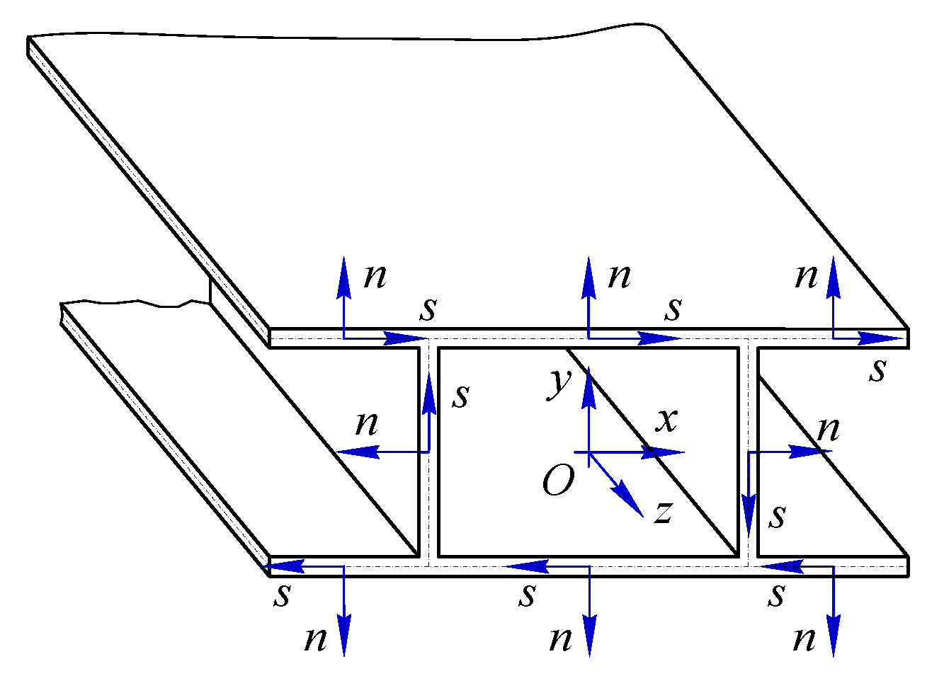
2. A Higher Order Model
2.1. Displacement Field
2.2. Governing Equations
3. Identification of Deformation Modes
3.1. Preliminary Deformation Modes
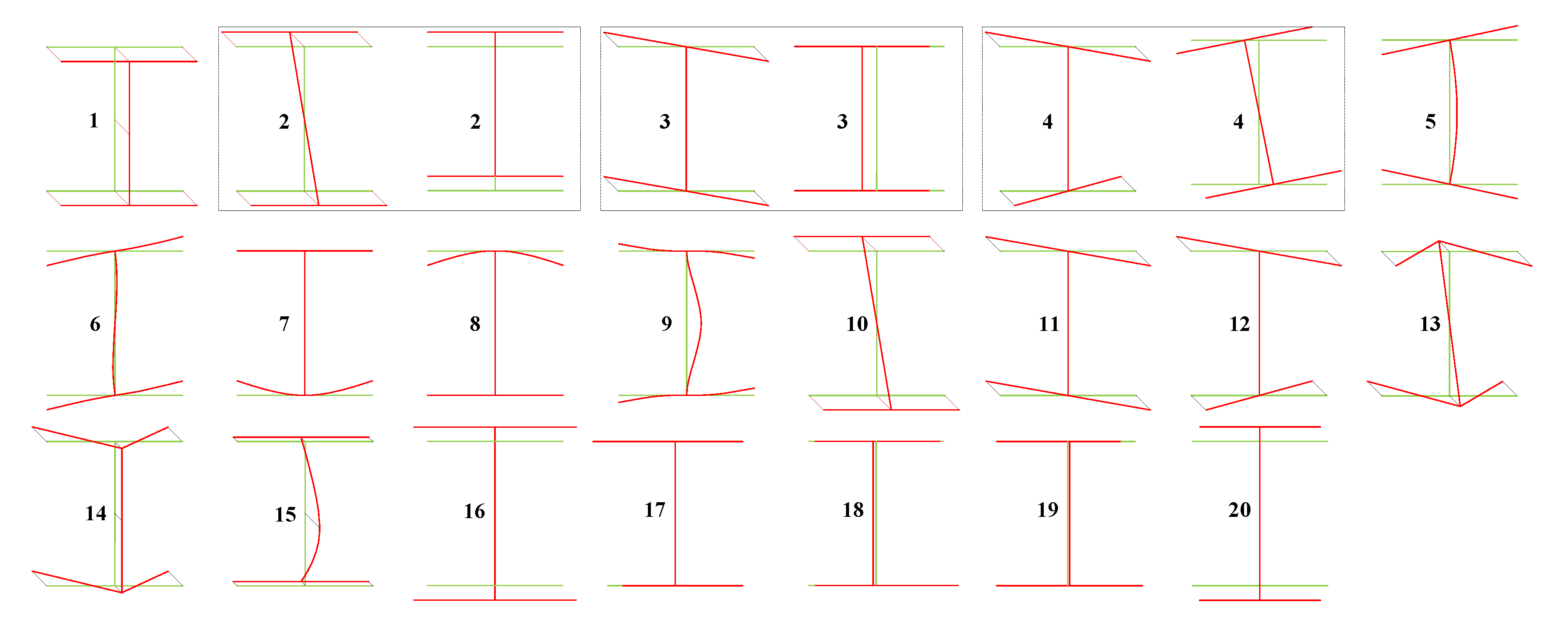
3.2. Cross-Section Deformation Modes
3.2.1. Basic Algorithms
3.2.2. Concrete Implementation
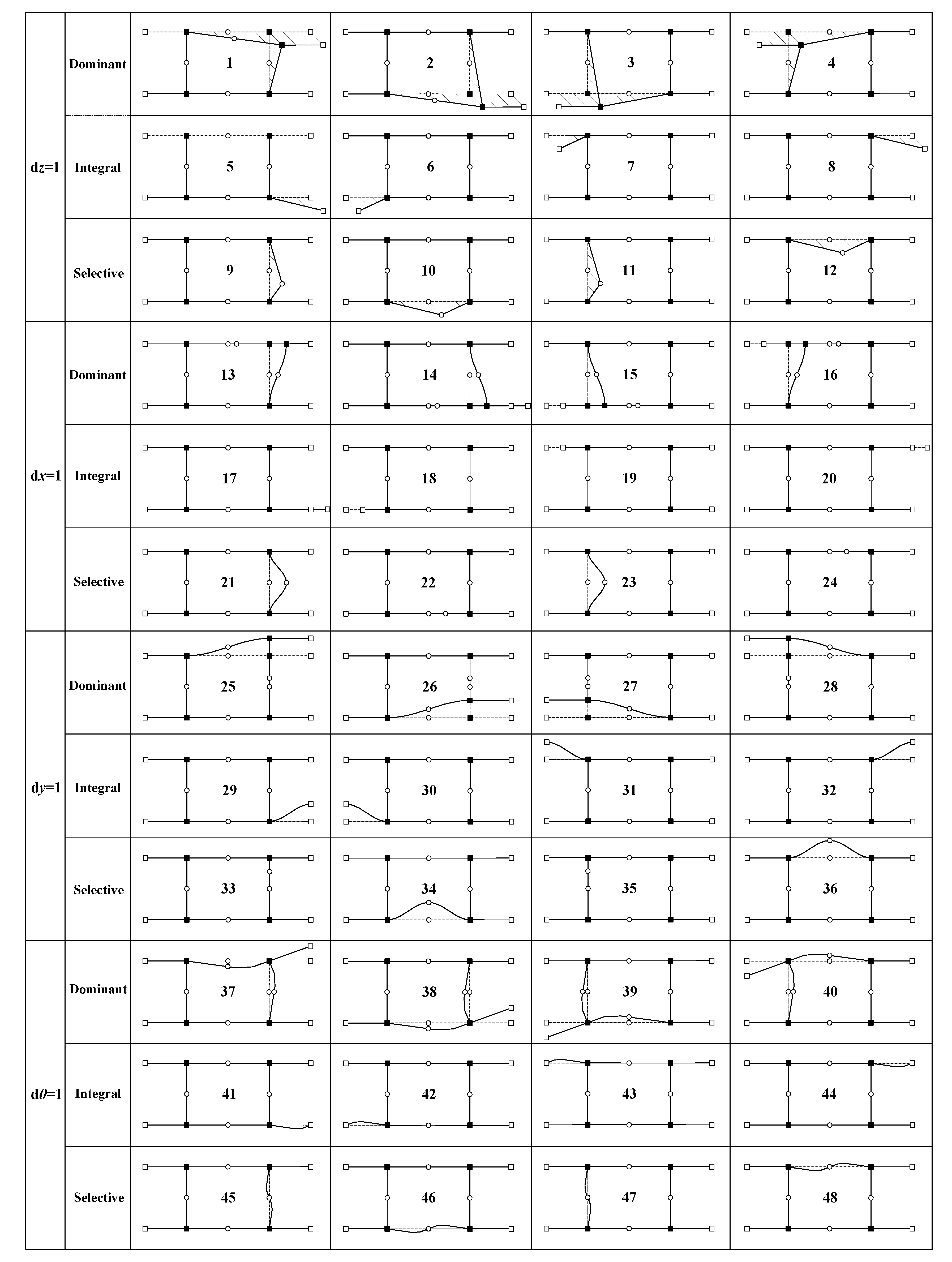
3.2.3. Numbering of Identified Deformation Modes
4. Illustrative Examples
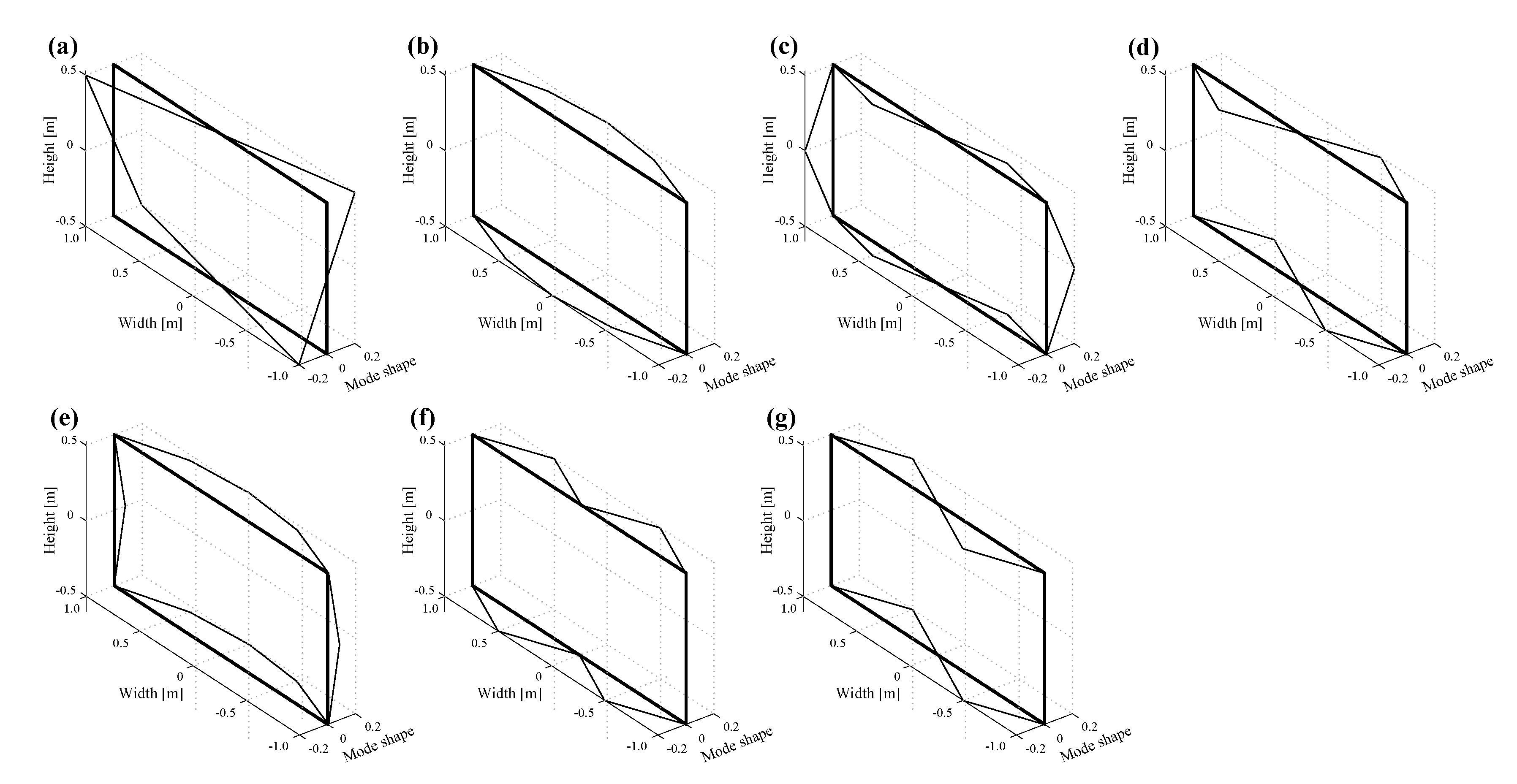
4.1. Cross-Section Analysis
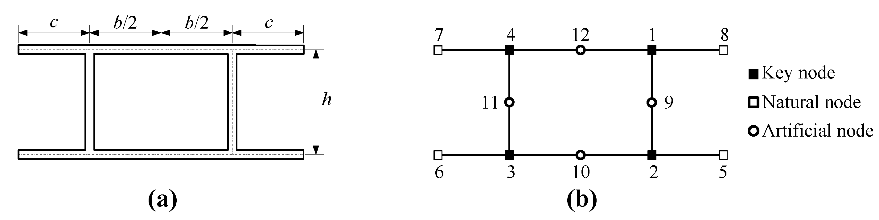
4.1.1. An I-Shaped Cross-Section
4.1.2. A Single-Cell Rectangular Cross-Section
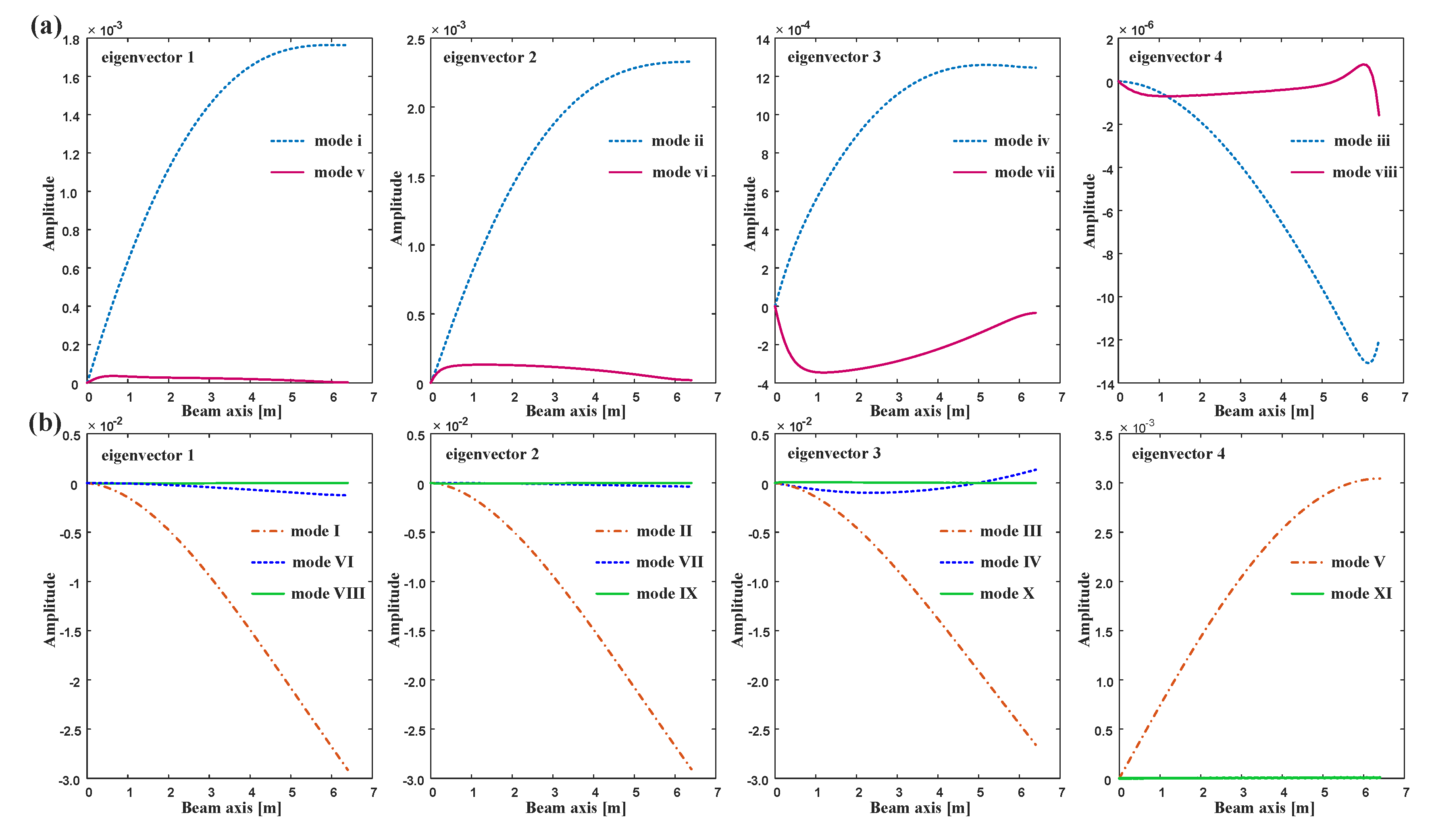
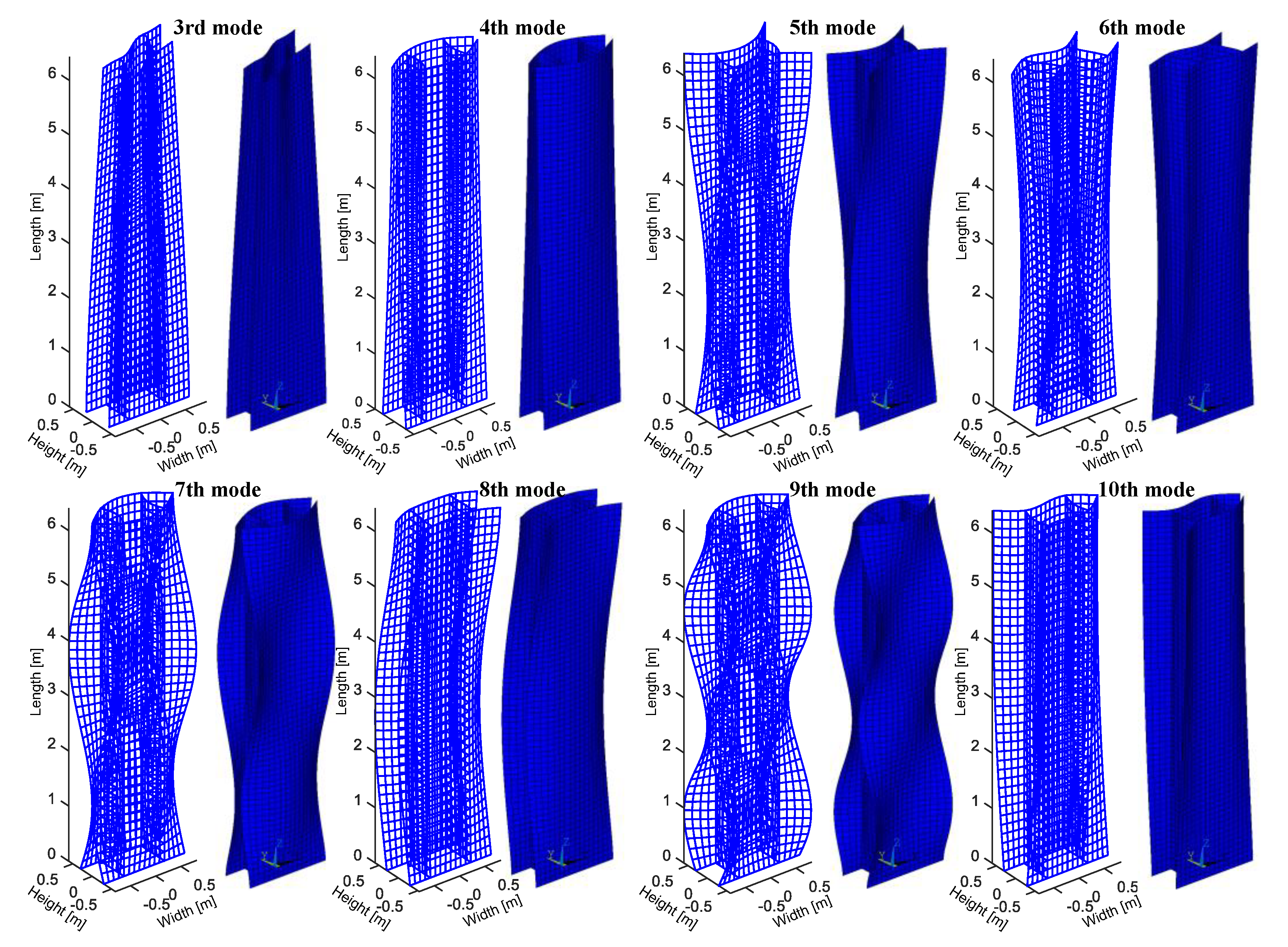
4.2. Beam Analysis
4.2.1. Concerning the Accuracy and Efficiency
4.2.2. Concerning the Reproduction of 3D Deformation
5. Conclusions
Author Contributions
Funding
Conflicts of Interest
References
- Yang, Z.; Xu, C. Research on Compression Behavior of Square Thin-Walled CFST Columns with Steel-Bar Stiffeners. Appl. Sci. 2018, 8, 1602. [Google Scholar] [CrossRef]
- El Fatmi, R. A refined 1D beam theory built on 3D Saint-Venant’s solution to compute homogeneous and composite beams. J. Mech. Mater. Struct. 2016, 11, 345–378. [Google Scholar] [CrossRef]
- Genoese, A.; Genoese, A.; Bilotta, A.; Garcea, G. A geometrically exact beam model with non-uniform warping coherently derived from the Saint Venant rod. Eng. Struct. 2014, 68, 33–46. [Google Scholar] [CrossRef]
- Naccache, F.; El Fatmi, R. Buckling analysis of homogeneous or composite I-beams using a 1D refined beam theory built on Saint Venant’s solution. Thin Walled Struct. 2018, 127, 822–831. [Google Scholar] [CrossRef]
- Naccache, F.; El Fatmi, R. Numerical free vibration analysis of homogeneous or composite beam using a refined beam theory built on Saint Venant’s solution. Comput. Struct. 2018, 210, 102–121. [Google Scholar] [CrossRef]
- Carrera, E.; Pagani, A.; Petrolo, M.; Zappino, E. Recent developments on refined theories for beams with applications. Mech. Eng. Rev. 2015, 2. [Google Scholar] [CrossRef]
- Berdichevskii, V. Variational-asymptotic method of constructing a theory of shells. J. Appl. Math. Mech. 1979, 43, 711–736. [Google Scholar] [CrossRef]
- Zhang, L.; Sertse, H.M.; Yu, W. Variational asymptotic homogenization of finitely deformed heterogeneous elastomers. Compos. Struct. 2019, 216, 379–391. [Google Scholar] [CrossRef]
- Harursampath, D.; Harish, A.B.; Hodges, D.H. Model reduction in thin-walled open-section composite beams using variational asymptotic method. Part I: Theory. Thin Walled Struct. 2017, 117, 356–366. [Google Scholar] [CrossRef]
- Jiang, F.; Deo, A.; Yu, W. A composite beam theory for modeling nonlinear shear behavior. Eng. Struct. 2018, 155, 73–90. [Google Scholar] [CrossRef]
- Carrera, E.; Petrolo, M. On the effectiveness of higher-order terms in refined beam theories. J. Appl. Mech. 2011, 78, 021013. [Google Scholar] [CrossRef]
- Pagani, A.; Yan, Y.; Carrera, E. Exact solutions for static analysis of laminated, box and sandwich beams by refined layer-wise theory. Compos. Part B Eng. 2017, 131, 62–75. [Google Scholar] [CrossRef]
- Yan, Y.; Pagani, A.; Carrera, E. Exact solutions for free vibration analysis of laminated, box and sandwich beams by refined layer-wise theory. Compos. Struct. 2017, 175, 28–45. [Google Scholar] [CrossRef]
- Carrera, E.; Pagani, A.; Banerjee, J.R. Linearized buckling analysis of isotropic and composite beam-columns by Carrera Unified Formulation and Dynamic Stiffness Method. Mech. Adv. Mater. Struct. 2016, 23, 1092–1103. [Google Scholar] [CrossRef]
- Yan, Y.; Carrera, E.; De Miguel, A.; Pagani, A.; Ren, Q.W.; Miguel, A. Meshless analysis of metallic and composite beam structures by advanced hierarchical models with layer-wise capabilities. Compos. Struct. 2018, 200, 380–395. [Google Scholar] [CrossRef]
- Vlassov, V. Thin-Walled Elastic Beams; Israel Program for Scientific Translations: Jerusalem, Israel, 1961. [Google Scholar]
- Capdevielle, S.; Grange, S.; Dufour, F.; Desprez, C. A multifiber beam model coupling torsional warping and damage for reinforced concrete structures. Eur. J. Environ. Civ. Eng. 2016, 20, 914–935. [Google Scholar] [CrossRef]
- Yoon, K.; Lee, P.S.; Kim, D.N. An efficient warping model for elastoplastic torsional analysis of composite beams. Compos. Struct. 2017, 178, 37–49. [Google Scholar] [CrossRef]
- Lim, T.C. Refined shear correction factor for very thick simply supported and uniformly loaded isosceles right triangular auxetic plates. Smart Mater. Struct. 2016, 25, 54001. [Google Scholar] [CrossRef]
- Pavazza, R.; Blagojevic, B. On the cross-section distortion of thin-walled beams with multi-cell cross-sections subjected to bending. Int. J. Solids Struct. 2005, 42, 901–925. [Google Scholar] [CrossRef]
- Park, N.H.; Choi, S.; Kang, Y.J. Exact distortional behavior and practical distortional analysis of multicell box girders using an expanded method. Comput. Struct. 2005, 83, 1607–1626. [Google Scholar] [CrossRef]
- Cambronero-Barrientos, F.; Díaz-Del-Valle, J.; Martínez-Martínez, J.A. Beam element for thin-walled beams with torsion, distortion, and shear lag. Eng. Struct. 2017, 143, 571–588. [Google Scholar] [CrossRef]
- Zhang, Y.H.; Lin, L.X. Shear lag analysis of thin-walled box girders based on a new generalized displacement. Eng. Struct. 2014, 61, 73–83. [Google Scholar] [CrossRef]
- Schardt, R. Generalized beam theory—An adequate method for coupled stability problems. Thin Walled Struct. 1994, 19, 161–180. [Google Scholar] [CrossRef]
- Gonçalves, R.; Camotim, D.; Peres, N. Application of Generalised Beam Theory to curved members with circular axis. Stahlbau 2018, 87, 345–354. [Google Scholar] [CrossRef]
- Gonçalves, R.; Camotim, D. On the first-order and buckling behaviour of thin walled regular polygonal tubes. Steel Constr. 2016, 9, 279–290. [Google Scholar] [CrossRef]
- Bebiano, R.; Basaglia, C.; Camotim, D.; Gonçalves, R. GBT buckling analysis of generally loaded thin-walled members with arbitrary flat-walled cross-sections. Thin Walled Struct. 2018, 123, 11–24. [Google Scholar] [CrossRef]
- Bebiano, R.; Eisenberger, M.; Camotim, D.; Gonçalves, R. GBT-Based Vibration Analysis Using the Exact Element Method. Int. J. Struct. Stab. Dyn. 2018, 18, 1850068. [Google Scholar] [CrossRef]
- Ruggerini, A.; Madeo, A.; Gonçalves, R.; Camotim, D.; Ubertini, F.; De Miranda, S. GBT post-buckling analysis based on the Implicit Corotational Method. Int. J. Solids Struct. 2019, 163, 40–60. [Google Scholar] [CrossRef]
- Bebiano, R.; Calçada, R.; Camotim, D.; Silvestre, N. Dynamic analysis of high-speed railway bridge decks using generalised beam theory. Thin Walled Struct. 2017, 114, 22–31. [Google Scholar] [CrossRef]
- Vieira, R.; Virtuoso, F.; Pereira, E. A higher order beam model for thin-walled structures with in-plane rigid cross-sections. Eng. Struct. 2015, 84, 1–18. [Google Scholar] [CrossRef]
- Vieira, R.; Virtuoso, F.; Pereira, E. Buckling of thin-walled structures through a higher order beam model. Comput. Struct. 2017, 180, 104–116. [Google Scholar] [CrossRef]
- Vieira, R.; Virtuoso, F.; Pereira, E. Definition of warping modes within the context of a higher order thin-walled beam model. Comput. Struct. 2015, 147, 68–78. [Google Scholar] [CrossRef]
- Vieira, R.F.; Virtuoso, F.; Pereira, E.; Virtuoso, F. A higher order model for thin-walled structures with deformable cross-sections. Int. J. Solids Struct. 2014, 51, 575–598. [Google Scholar] [CrossRef]
- Zhang, L.; Zhu, W.; Ji, A.; Peng, L. A Simplified Approach to Identify Sectional Deformation Modes of Thin-Walled Beams with Prismatic Cross-Sections. Appl. Sci. 2018, 8, 1847. [Google Scholar] [CrossRef]
- Bebiano, R.; Gonçalves, R.; Camotim, D. A cross-section analysis procedure to rationalise and automate the performance of GBT-based structural analyses. Thin Walled Struct. 2015, 92, 29–47. [Google Scholar] [CrossRef]
- Zhang, L.; Ji, A.; Zhu, W.; Peng, L. On the Identification of Sectional Deformation Modes of Thin-Walled Structures with Doubly Symmetric Cross-Sections Based on the Shell-Like Deformation. Symmetry 2018, 10, 759. [Google Scholar] [CrossRef]
- Bebiano, R.; Camotim, D.; Gonçalves, R. GBTul 2.0—A second-generation code for the GBT-based buckling and vibration analysis of thin-walled members. Thin Walled Struct. 2018, 124, 235–257. [Google Scholar] [CrossRef]


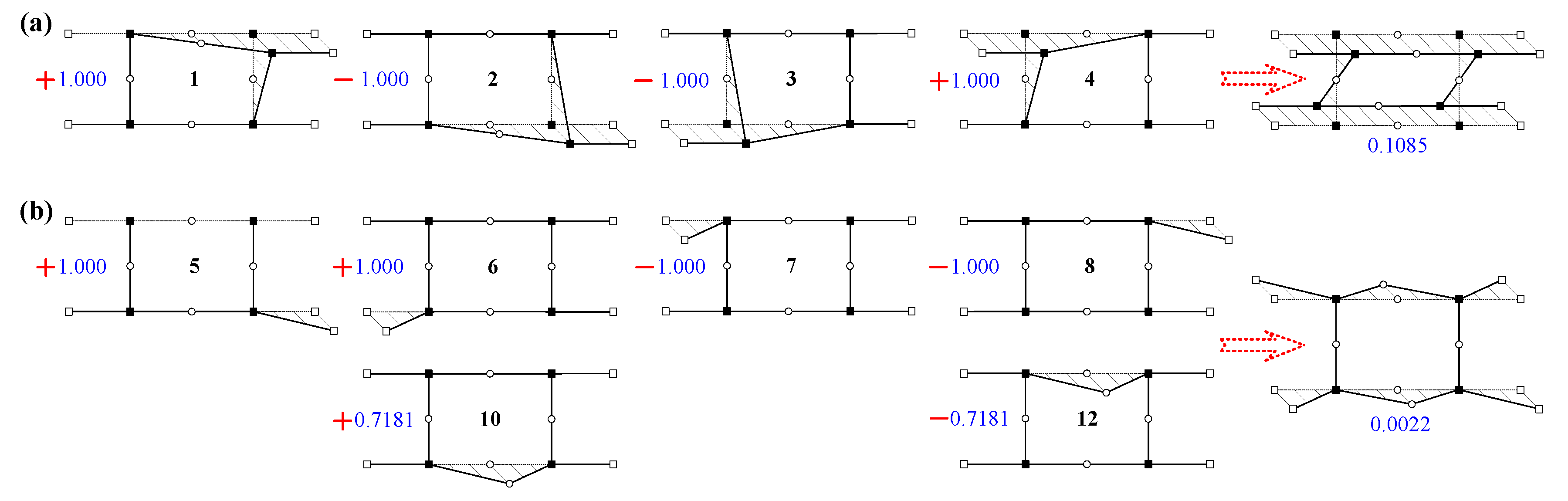
| PDM i | Participation ξi | Correlation Coefficient r1,j | Weight λ1,j | Residual Participation ξi | Correlation Coefficient r5,j | Weight λ5,j | Residual Participation ξi |
|---|---|---|---|---|---|---|---|
| 1 | 0.1085 | 1 | 1 | 0 | / | / | 0 |
| 2 | 0.1085 | −1.000 | −1.000 | 0 | / | / | 0 |
| 3 | 0.1085 | −1.000 | −1.000 | 0 | / | / | 0 |
| 4 | 0.1085 | 1.000 | 1.000 | 0 | / | / | 0 |
| 5 | 0.0022 | / | / | 0.0022 | 1 | 1 | 0 |
| 6 | 0.0022 | / | / | 0.0022 | 1.000 | 1.000 | 0 |
| 7 | 0.0022 | / | / | 0.0022 | −1.000 | −1.000 | 0 |
| 8 | 0.0022 | / | / | 0.0022 | −1.000 | −1.000 | 0 |
| 11 | 0.0017 | / | / | 0.0017 | 0.5874 | 0.7181 | 0.0004 |
| 12 | 0.0017 | / | / | 0.0017 | −0.5874 | −0.7181 | 0.0004 |
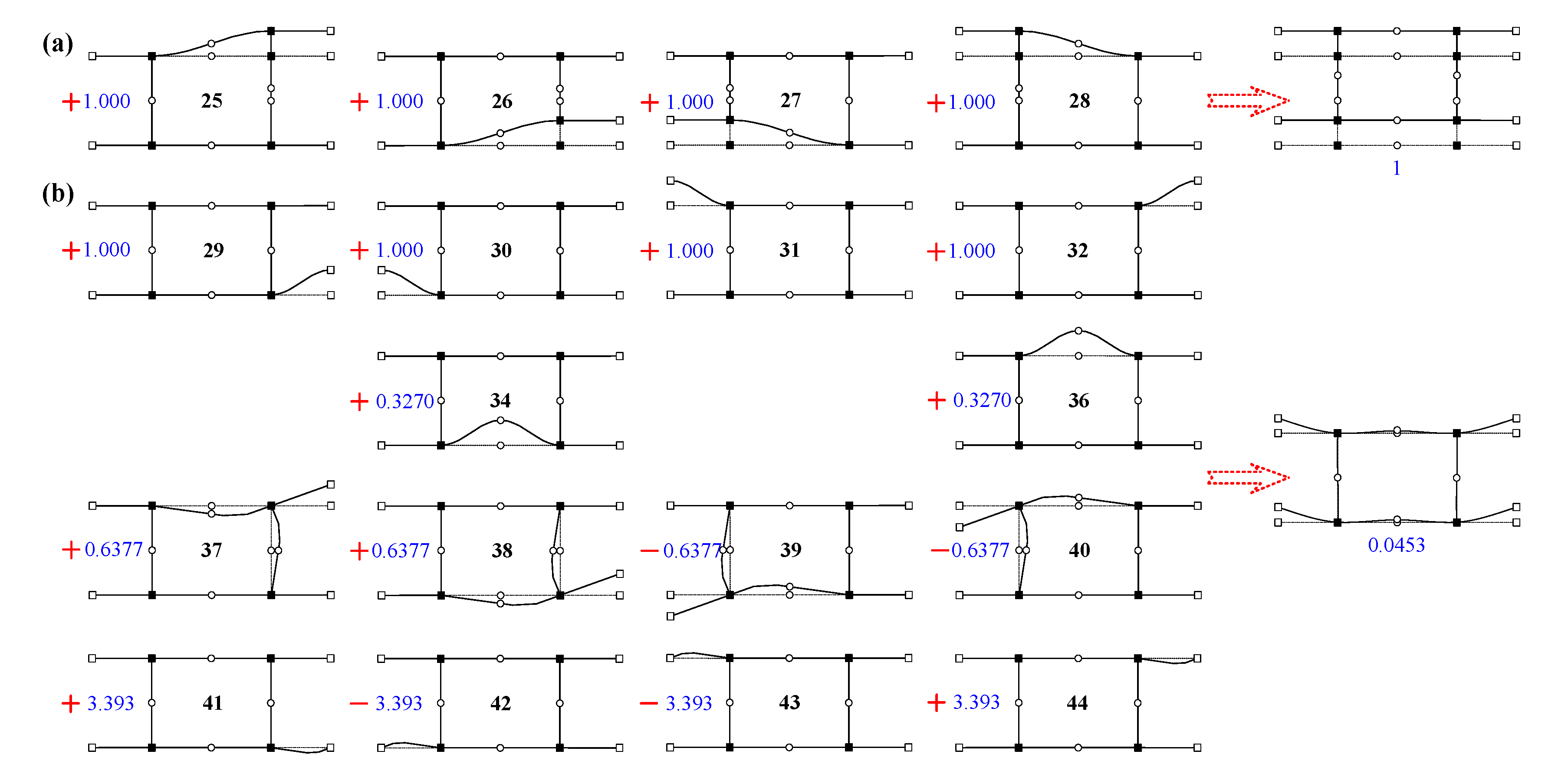
| PDM i | Participation ξi | Correlation Coefficient r29,j | Weight λ29,j | Residual Participation ξi | Correlation Coefficient r13,j | Weight λ13,j | Residual Participation ξi |
|---|---|---|---|---|---|---|---|
| 29 | 0.0453 | 1 | 1 | 0 | / | / | / |
| 34 | 0.0147 | 0.9997 | 0.3270 | 0.0004 | / | / | / |
| 37 | 0.0291 | 0.9959 | 0.6377 | 0.0059 | −0.9935 | −2.274 | 0.0016 |
| 39 | 0.0291 | −0.9959 | −0.6377 | 0.0059 | 0.9935 | 2.274 | 0.0016 |
| 41 | 0.1547 | 0.9995 | 3.393 | 0.0002 | / | / | / |
| 13 | 0.0024 | / | / | 0.0024 | 1 | 1 | 0 |
| 14 | 0.0024 | / | / | 0.0024 | −1.000 | −1.000 | 0 |
| 17 | 0.0026 | / | / | 0.0026 | −1.000 | −1.000 | 0 |
| 18 | 0.0026 | / | / | 0.0026 | 1.000 | 1.000 | 0 |
| 33 | 0.0010 | / | / | 0.0010 | −0.9062 | −0.4038 | 0.0002 |
| Mode Number | ANSYS Shell | Proposed Beam 1 | Classic Beam | Proposed Beam 2 | Proposed Beam 3 | Proposed Beam 4 | |||||
|---|---|---|---|---|---|---|---|---|---|---|---|
| Frequency [Hz] | Frequency [Hz] | Relative Error [%] | Frequency [Hz] | Relative Error [%] | Frequency [Hz] | Relative Error [%] | Frequency [Hz] | Relative Error [%] | Frequency [Hz] | Relative Error [%] | |
| 1 | 17.83 | 17.91 | 0.45 | 18.77 | 5.27 | 18.66 | 4.65 | 18.57 | 4.15 | 18.48 | 3.64 |
| 2 | 29.01 | 29.16 | 0.52 | 30.63 | 5.58 | 30.43 | 4.89 | 30.35 | 4.62 | 30.16 | 3.96 |
| 3 | 43.20 | 42.56 | −1.48 | 77.52 | 79.4 | 44.11 | 2.11 | 44.11 | 2.11 | 43.20 | 0 |
| 4 | 57.73 | 56.97 | −1.32 | / | / | 57.11 | −1.07 | 57.11 | −1.07 | 57.11 | −1.07 |
| 5 | 60.56 | 58.86 | −2.81 | / | / | 59.89 | −1.11 | 59.89 | −1.11 | 59.89 | −1.11 |
| 6 | 65.10 | 63.74 | −2.09 | / | / | / | / | / | / | 64.23 | −1.34 |
| 7 | 66.62 | 64.69 | −2.90 | / | / | 65.13 | −2.24 | 65.13 | −2.24 | 65.13 | −2.24 |
| 8 | 72.53 | 72.01 | −0.72 | / | / | 72.30 | −0.32 | 72.30 | −0.32 | 72.30 | −0.32 |
| 9 | 75.31 | 76.27 | 1.27 | / | / | / | / | 78.34 | 4.02 | 78.20 | 3.84 |
| 10 | 75.71 | 76.95 | 1.64 | / | / | / | / | 78.84 | 4.13 | 78.84 | 4.13 |
© 2019 by the authors. Licensee MDPI, Basel, Switzerland. This article is an open access article distributed under the terms and conditions of the Creative Commons Attribution (CC BY) license (http://creativecommons.org/licenses/by/4.0/).
Share and Cite
Zhang, L.; Ji, A.; Zhu, W. A Novel Approach to Perform the Identification of Cross-Section Deformation Modes for Thin-Walled Structures in the Framework of a Higher Order Beam Theory. Appl. Sci. 2019, 9, 5186. https://doi.org/10.3390/app9235186
Zhang L, Ji A, Zhu W. A Novel Approach to Perform the Identification of Cross-Section Deformation Modes for Thin-Walled Structures in the Framework of a Higher Order Beam Theory. Applied Sciences. 2019; 9(23):5186. https://doi.org/10.3390/app9235186
Chicago/Turabian StyleZhang, Lei, Aimin Ji, and Weidong Zhu. 2019. "A Novel Approach to Perform the Identification of Cross-Section Deformation Modes for Thin-Walled Structures in the Framework of a Higher Order Beam Theory" Applied Sciences 9, no. 23: 5186. https://doi.org/10.3390/app9235186
APA StyleZhang, L., Ji, A., & Zhu, W. (2019). A Novel Approach to Perform the Identification of Cross-Section Deformation Modes for Thin-Walled Structures in the Framework of a Higher Order Beam Theory. Applied Sciences, 9(23), 5186. https://doi.org/10.3390/app9235186