Article

Tempo and Metrical Analysis by Tracking Multiple Metrical Levels Using Autocorrelation

by
Olivier Lartillot
1,* and
Didier Grandjean
2
1
RITMO Centre for Interdisciplinary Studies in Rhythm, Time and Motion, University of Oslo, 0318 Oslo, Norway
2
Department of Psychology, Swiss Center for Affective Sciences, University of Geneva, 1205 Geneva, Switzerland
*
Author to whom correspondence should be addressed.
Appl. Sci. 2019, 9(23), 5121; https://doi.org/10.3390/app9235121
Submission received: 30 September 2019 / Revised: 17 November 2019 / Accepted: 22 November 2019 / Published: 26 November 2019
(This article belongs to the Special Issue Sound and Music Computing -- Music and Interaction)

Abstract

:
We present a method for tempo estimation from audio recordings based on signal processing and peak tracking, and not depending on training on ground-truth data. First, an accentuation curve, emphasizing the temporal location and accentuation of notes, is based on a detection of bursts of energy localized in time and frequency. This enables the detection of notes in dense polyphonic texture, while ignoring spectral fluctuation produced by vibrato and tremolo. Periodicities in the accentuation curve are detected using an improved version of autocorrelation function. Hierarchical metrical structures, composed of a large set of periodicities in pairwise harmonic relationships, are tracked over time. In this way, the metrical structure can be tracked even if the rhythmical emphasis switches from one metrical level to another. This approach, compared to all the other participants to the Music Information Retrieval Evaluation eXchange (MIREX) Audio Tempo Extraction competition from 2006 to 2018, is the third best one among those that can track tempo variations. While the two best methods are based on machine learning, our method suggests a way to track tempo founded on signal processing and heuristics-based peak tracking. Moreover, the approach offers for the first time a detailed representation of the dynamic evolution of the metrical structure. The method is integrated into MIRtoolbox, a Matlab toolbox freely available.

Graphical Abstract

1. Introduction

Detecting tempo in music and tracking the evolution of tempo over time is a topic of research in Music Information Retrieval (MIR) that has been extensively studied in recent decades. Recent approaches based on deep learning have contributed to an important progress in the state of the art [1,2]. In this paper, we present a method that relates to a more classical approach based on signal processing and heuristics-based data extraction. This classical approach generally detects in a first step the temporal repartition of notes, leading to an accentuation curve (or onset detection curve) that is further analyzed, in a second step, for periodicity estimation.
The new proposed method is aimed at improving on those successive steps constituting the classical approach. First, a method for accentuation curve is developed, based on a detection of bursts of energy localized in time and frequency. This enables better emphasis of notes in dense polyphonic texture, while ignoring spectral fluctuation produced by vibrato and tremolo. Second, periodicity detection is performed using an improved version of autocorrelation function. Finally, hierarchical metrical structures, composed of a large set of periodicities in pairwise harmonic relationships, are tracked over time in parallel. In this way, the metrical structure can be tracked even if the rhythmical emphasis switches from one metrical level to another. A selection of core metrical levels enables the estimation of meter and tempo. Moreover, the tracking along many metrical levels in parallel enables a detailed description of the dynamic evolution of the metrical structure: not only how the whole structure speeds up or slows down with respect to global tempo, but also how individual metrical levels might be emphasized at particular moments in the music. To provide an indication of metrical activity that would not focus solely on tempo, we introduce a new measure, called dynamic metrical centroid, which takes into consideration the rhythmical activity at the various metrical levels. The overall structure of the proposed method is schematized in Figure 1.
This approach, compared to all the other participants to the Music Information Retrieval Evaluation eXchange (MIREX) Audio Tempo Extraction competition from 2006 to 2018, is the third best one among those that can track tempo variations. While the two best methods are based on machine learning, our method suggests a way to track tempo founded on signal processing and heuristics-based peak tracking.
We previously briefly presented the principles of the approach [3] and more recently described the method in more details [4]. This paper discusses the state of the art in more details, provides a more detailed and accurate description of the proposed method, and provides an extended bibliography of the MIREX Audio Tempo Extraction competition [5].

2. Related Work

2.1. Accentuation Curve

The estimation of tempo starts from a temporal description of the location and strength of events appearing in the piece of music, leading to an “onset detection curve”, also called accentuation curve [6]. Musical events are indicated by peaks; the height of each peak is related to the importance of the related event.

2.1.1. Classical Methods

The various methods for estimation of this accentuation curve mainly differ in the way this energy or difference of energy is observed. Envelope-based approaches globally estimate the energy for each successive temporal frame without considering its spectral decomposition along frequencies; spectral-flux methods estimate the difference of energy over successive frames on individual frequencies, and further summed together [7,8]. Both approaches would work in the case of sequences made of notes sufficiently isolated or accentuated with respect to the background, corresponding to short bursts of energy separated by low-energy transitions, as in simple percussive sequences. Indeed, in such case, the resulting envelope and spectral flux would show each percussive event with a peak. This can be seen for instance, in Figure 2, on the left side.
On the contrary, for dense musical sequences featuring overlapped notes, such as complex orchestral sounds, the spectral-flux method better distinguishes the attack of individual notes, provided that the different notes occupy distinct frequency bands. Minor energy fluctuation along particular frequencies may blur the resulting accentuation curve, hindering the detection of note attacks. The use of thresholding can filter out energy fluctuation on constant frequency bands (such as tremolo) so that only significantly high energy bursts related to note attacks are selected. Still, energy fluctuating in frequency, such as vibrato, may still add noise to the resulting accentuation curve. This can be seen in Figure 2, on the right side.

2.1.2. Localized Methods

To detect significant energy bursts on highly localized frequency ranges but still filter out the artifacts due to the possible frequency fluctuation along time of such localized events, it is necessary to add some tracking capability. The approach presented by [9] can be considered to be an answer to this problem. From a spectrogram of frame length 46.44 ms (frequency resolution 21.53 Hz) and hop 11.61 ms, rapid increases of amplitude are searched for on individual frequency components. For each detected onset is evaluated its “degree of onset", defined as the rapidity of increase in amplitude.
More precisely the method searches for particular frequency components f at a particular time frame t, where the two following conditions are reached:
  • The power of the spectral component at frequency f and time t, denoted p ( t , f ) , is higher than the power around the previous time frame at similar frequency:
    p ( t , f ) > p p ( t , f )
    where p p is defined as follows:
    p p ( t , f ) = max max f [ f 1 , f + 1 ] p ( t 1 , f ) , p ( t 2 , f )
    We propose to call this time-frequency region associated with p p ( t , f ) contextual background at time t and frequency f. This is illustrated in Figure 3.
  • The power at next time frame and similar frequency n p is higher than the power in the contextual background:
    n p ( t , f ) > p p ( t , f )
    where n p is given by the following definition:
    n p ( t , f ) = min f [ f 1 , f + 1 ] p ( t + 1 , f )
If p is an onset, its degree of onset is given by
d o ( t , f ) = max ( p ( t , f ) , p ( t + 1 , f ) ) p p ( t , f )
For a given instant t, the degrees of onset are summed over the frequency components, resulting in an onset curve.

2.2. Periodicity Analysis

A pulsation corresponds to a periodicity in the succession of peaks in the accentuation curve. Classical signal-processing methods estimate periodicity using methods such as autocorrelation, YIN [10], bank of comb-filter resonators with a constant half-time [11] or phase-locking resonators [12]. (Cf. [6] for a detailed literature review.) Basically, a range of possible periodicity frequencies is considered, and for each frequency, periodicity is searched for.
Klapuri et al. consider that “the key problems in meter analysis are in measuring the degree of musical accentuation and in modeling higher-level musical knowledge, not in finding exactly the correct period estimator” [6]. They point out however a specific feature offered using a bank of comb-filter resonators, namely that high scores are given not only to the actual periods expressed in the input accentuation curve, but also to subharmonics of these periods. For instance, for a simple pulse of period 1 s—corresponding to a tempo of 60 beats per minute (BPM)—all methods (autocorrelation function, bank of resonators) give high scores to periods related to 1 s and all its multiples: 2 s (30 BPM), 3 s (20 BPM), etc.; but bank of resonators also give high scores to subharmonics such as 0.5 s (120 BPM), 0.33 s (180 BPM), 0.25 and 0.75 s, etc. In our view, the addition of hypothetical faster pulsations are not informative if they do not explicitly appear in the input sequence, and especially if they could contradict with the actual metrical structure.
On the other hand, one main disadvantage of autocorrelation function is the fact that it does not explicitly look for periodic events in the input sequence of period T, but only to the prominence of pairs of high values in the input sequences separated by the duration T. Periodic sequences of period T lead to high prominence of duration T, but the reverse is not true: pairs of pulses of duration T can populate a sequence without being necessarily periodic. For instance, a 4-beat periodic pattern with accentuation of the first and fourth beat leads to a high score for the 4-beat period, but also for the 3-beat period, although the latter is not periodic. We propose in Section 3.2 a way to filter out these non-periodic high scores in the autocorrelation function.
In the following, we will call periodicity function the representation, such as autocorrelation function, showing the periodicity score related to each possible period (also called lag in autocorrelation functions) expressed in seconds, or alternatively each possible frequency in Hz. Since the analysis is performed on a moving window, all periodicity functions can be grouped into one representation called periodogram. If the periodicity function is an autocorrelation function, this can be also called autocorrelogram. An example of autocorrelogram is shown in Figure 4, where each column displays an autocorrelation function computed on a time window of 5 s, which progressively scans the audio recording from beginning to end.
It has been asserted that accentuation curves need to be estimated on several distinct registers—5 according to Scheirer [11] and Klapuri suggest even up to 40 different bands [6]—and that periodicity needs to be estimated on each register separately. This method would particularly work in the case of complex musical examples where the main pulsation can be extracted on a particular register frequency region. This multi-band strategy was possibly designed to counteract some limitations of the classical methods for accentuation curve: because they fail to produce clear accentuation curves for complex polyphony, a decomposition into frequency bands might produce clearer accentuation curves. However, for musical examples where the pulsation is scattered along various frequency bands, this method would not offer any particular advantage and could even fail to catch that periodicity.

2.3. Metrical Structure

In the presence of a given pulsation in the musical excerpt that is being analyzed—let’s say with a BPM of 120, i.e., with two pulses per second—the periodicity function will indicate a high periodicity score related to the period 0.5 s. But generally, as previously discussed, if there is a pulsation at a given tempo, multiples of the pulsation can also be found that are twice slower (1 s), three times slower, etc. For that reason, the periodicity function usually shows a series of peaks equally distant, corresponding to multiples of a given period. This can be seen for instance in Figure 4. This harmonicity of the rhythm periodicity has close connections with the notion of metrical structure in music, with a hierarchical ordering of rhythmical values such as whole notes, half notes, quarter notes, etc.
One common approach to extract tempo from the periodicity function is to select the highest peak, within a range of beat periodicities considered to be most adequate, typically between 40 and 200 BPM, with a weighted emphasis on a range of best perceived periodicities. Studies have designed so-called “resonance curves” that weight the periodicity score depending on the period, so that periods around 120 BPMs would be preferred [13,14]. This approach fails when tracking the temporal evolution of tempo over time, especially for pieces of music where different metrical levels are emphasized throughout the temporal development. For instance, if at a given moment of the piece of music, there is an accentuated quarter-note pulsation followed by an accentuated eighth-note pulsation, the tempo tracking will switch from one BPM value to another one twice faster, although the actual tempo might remain constant. And as we may imagine, such shift from one metrical level to another is very frequent in music. Figure 4 and Figure 5 show an example of analysis using this simple method.
In [6], three particular metrical levels are considered to be core elements of the metrical structure:
  • The tactus is considered to be the most prominent level, also referred as the foot-tapping rate or the beat. The tempo is often identified with the tactus level.
  • The tatum—for “temporal atom”—is considered to be the fastest subdivision of the metrical hierarchy, such that all other metrical levels (in particular tactus and bar) are multiples of that tatum.
  • The bar level or other metrical levels considered to be related to change of chords, melodic or rhythmic patterns, etc.
Klapuri et al. propose a method to track meter by modeling dependencies between successive instants [6]. In our view, one major interest of this approach is that it is based on a tracking of parallel metrical levels, namely the three main metrical levels discussed previously —tatum, tactus and bar level—which they propose to call respectively levels A, B and C. More precisely, the period associated with each of the three levels, τ A , τ B and τ C , are tracked in parallel along time, frame by frame. The proposed Hidden Markov Model is designed in such a way that the period at each level is conditioned by the period at the same level on the previous frame. Moreover, τ C is probabilistically constrained to be an integer multiple of τ B and τ B to be an integer multiple of τ A . Finally, the values of the three periods ( τ A , τ B , τ C ) at a given frame are also conditioned by the periodicity function s at that frame, in the form of a state-conditional observation likelihoods p ( s | τ A , τ B , τ C ) , which is evaluated from a database of musical recordings where the meter has been hand-labeled.
In our view, one main limitation of this approach is that the tracking is based on the existence of three definite metrical levels (tatum, tactus and bar level) that are supposed to stabilize on particular metrical levels. In a large range of music, there is not necessarily a clear emergence of three core levels. The tatum is considered (and modeled) as the minimal subdivision such that each other metrical level is a multiple of that elementary level, but this canonic situation does not describe all metrical cases: for instance, binary and ternary subdivisions often coexist, as we will see for instance in Section 5.
Another limitation of the use of a Hidden Markov Model is that this requires extensive training and specification of particular statistics, such as the prior period distribution for each metrical level (tatum, tactus and bar level) and the probability distribution of the transition between successive frames.

2.4. Deep-Learning Approaches
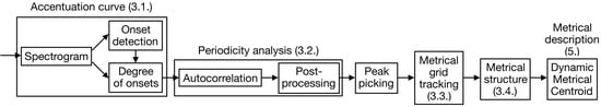
Recent deep-learning approaches start from the computation of a spectrogram, eventually followed by a filtering that emphasizes the contrast between successive frames, along each different frequency [1]. In [1], the successive frames of the spectrogram are then fed into a Bidirectional Long Short-Term Memory (BLSTM) Recurrent Neural Network (RNN). This network can be understood as performing both the detection of events based on local contrast and the detection of periodicity in the succession of events, along multiple metrical levels. This is followed by a Dynamic Bayesian Network that plays a similar role as the HMM, tracking pulsation along two metrical levels (corresponding to beats and downbeats). In [2], the whole process consists of feeding the spectrogram to a convolutional neural network (CNN).

3. Proposed Method

The proposed method introduces improvements in the successive steps forming the traditional procedure for metrical analysis presented in Section 2.1, Section 2.2, Section 2.3. A modification of the localized method for accentuation curve estimation enables better emphasis of note onsets in challenging audio recordings such as polyphony with vibrato and tremolo (Section 3.1). Periodicity detection is performed using a modified version of autocorrelation function (Section 3.2).
Moreover, we introduce a new methodology for tracking the metrical structure along a large range of periodicity layers in parallel. The tracking of the metrical structure is carried out in two steps:
  • a tracking of the metrical grid featuring a large range of possible periodicities (Section 3.3). Instead of considering a fix and small number of pre-defined metrical levels, we propose to track a larger range of periodicity layers in parallel.
  • a selection of core metrical levels, leading to a metrical structure, which enables the estimation of meter and tempo (Section 3.4).

3.1. Accentuation Curve

The proposed method for the inference of the accentuation curve follows the same general principle of the model introduced in [9], detecting and tracking the apparition of partials locally in the spectrogram, as explained in Section 2.1. In our case, the spectrogram is computed for the frequency range below 5000 Hz and the energy is represented in the logarithmic scale in decibel.
We use different parameters for the specification of the temporal scope and the frequency width of the contextual background. In [9], the frequency width is 43 Hz and the temporal depth 23 ms. After testing on a range of musical styles, we chose a frequency width of 17 Hz and a temporal depth of 40 ms (Figure 3). (The parameters indicated in our previous paper [4] were inaccurate.) By enlarging the temporal horizon of the contextual background, this enables filtration of tremolo effects and to focus on more prominent increase of energy.
In the proposed model, the second condition for onset detection specified in [9] —namely, that the energy on the frame succeeding the current one should be higher than the contextual background—is withdrawn, for the sake of simplicity. That constraint seems aimed at filtering out bursts of energy that are just one frame long, but bursts that are two frames long would not be filtered out. We might hypothesize that short bursts of energy might still be perceived as events.
Finally, the degree of onset is different from the one proposed in [9]. Instead of conditioning the degree of onset to the increase of energy with respect to the contextual background, we propose to condition it to the absolute level of energy:
d o ( t , f ) = p ( t , f )
This is because a burst of energy of a given level p ( t , f ) might be perceived as strong, and could contribute therefore to the detection of a note onset, even if there was a relatively loud sound in the frequency and temporal vicinity. This modification globally improved the results in our tests.
In our proposed method, the accentuation curve shows more note onsets than in [9]. This leads to a more detailed analysis of periodicity and a richer metrical analysis. This allows sometimes the discovery of the underlying metrical structure that was hidden under a complex surface and was not detected using [9].

3.2. Periodicity Analysis

Tempo is estimated by computing an autocorrelogram with a frame length of 5 s and hop factor 5%, for a range of time lags between 60 ms and 2.5 s, corresponding to a tempo range between 24 and 1000 BPM. The autocorrelation curve is normalized so that the autocorrelation at zero lag is identically 1.
A peak picking is applied to each frame of the autocorrelogram separately. The beginning and the end of the autocorrelation curves are not taken into consideration for peak picking as they do not correspond to actual local maxima. A given local maximum will be considered to be a peak if its distance with the previous and successive local minima (if any) is higher than 5% of the total amplitude range (i.e., the distance between the global maximum and minimum).
As discussed in Section 2.2, one important problem with autocorrelation functions is that a lag can be selected as prominent because it is found often in the signal although the lag is not repeated successively. We propose a simple solution based on the following property: For a given lag to be repeated at least twice, the periodicity score associated with twice the lag should have a high probability score as well. These heuristics can be implemented as a single post-processing operation applied to the autocorrelation function, removing any periodicity candidate for which there is no periodicity candidate at around twice its lag.

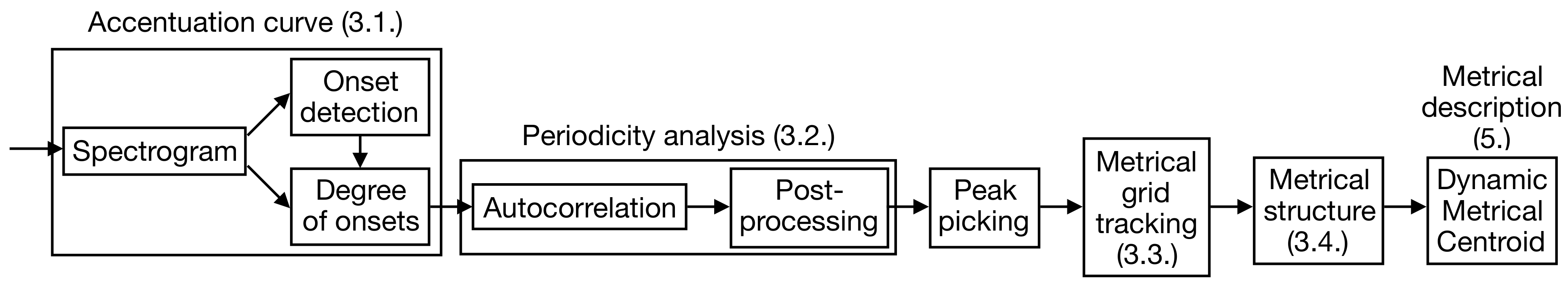
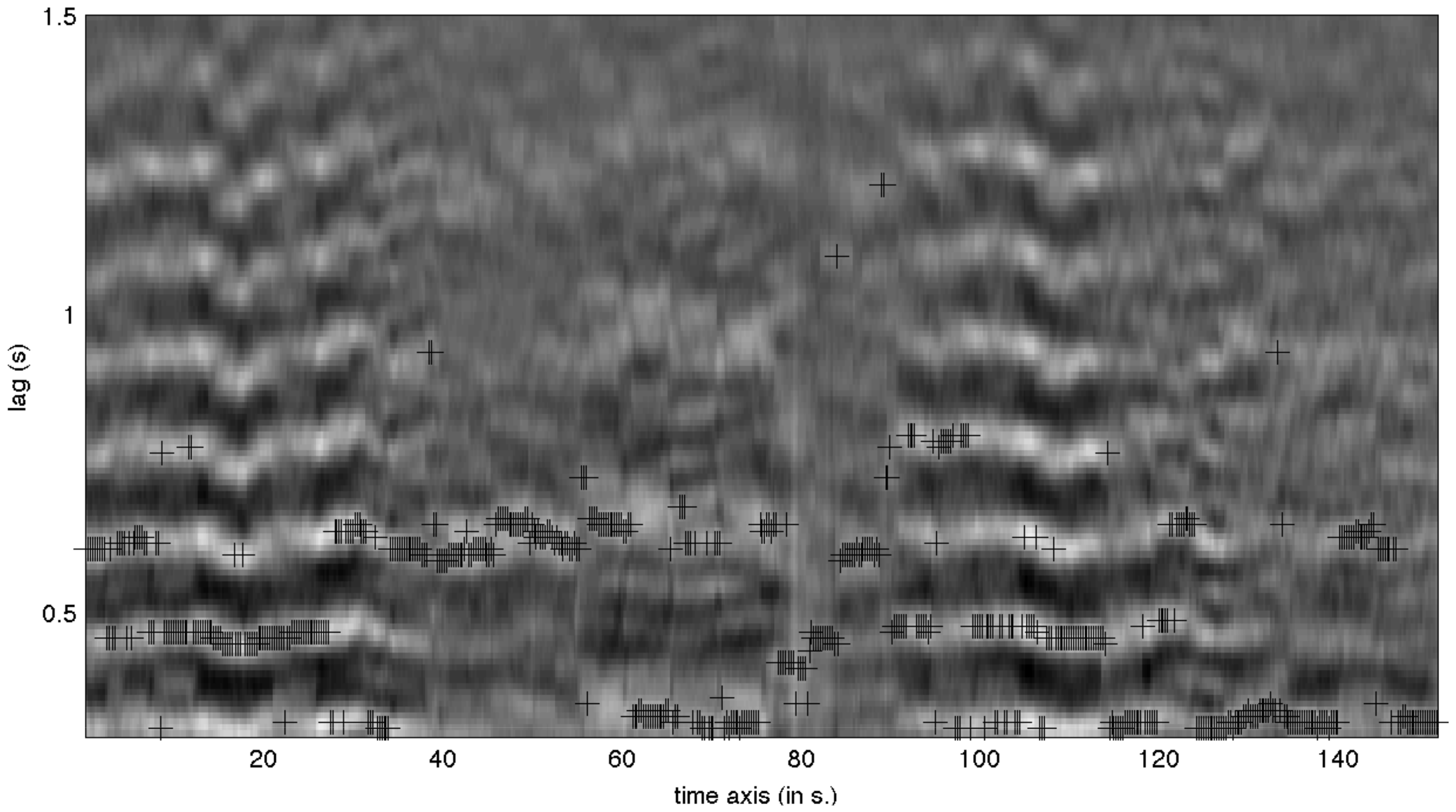
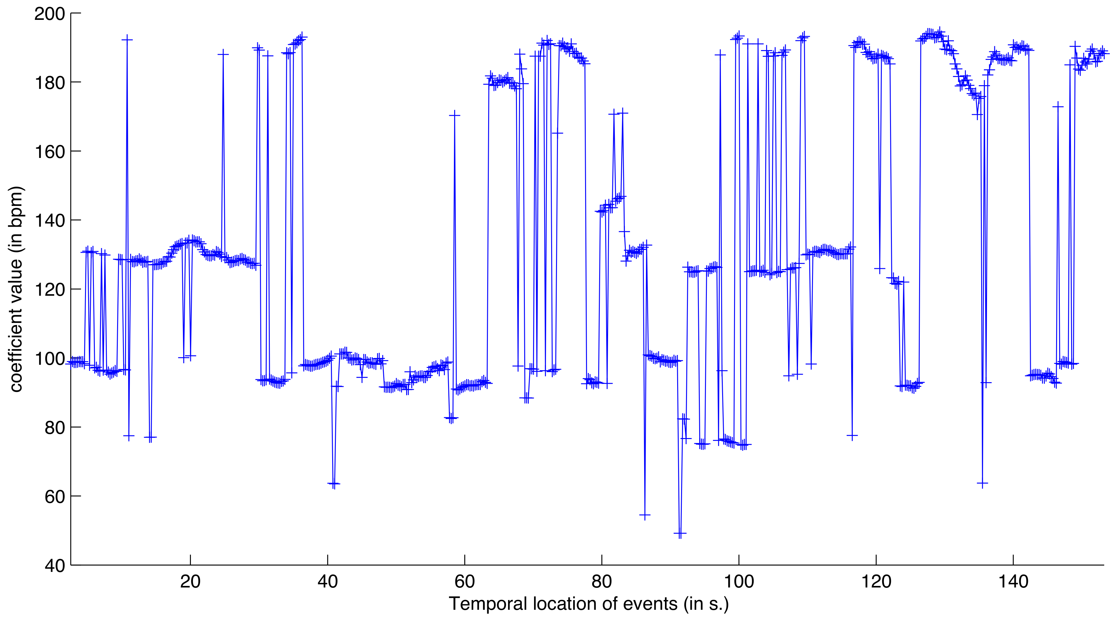
3.3. Tracking the Metrical Grid

The metrical structure is tracked over time along several metrical levels. But instead of focusing on three particular levels such as the decomposition tatum/tactus/bar level formalized in [6], we propose to consider the problem in a more general framework, by tracking virtually any possible periodicity layer in parallel.

3.3.1. Principles

The tracking of the metrical levels is done in two successive steps:
  • We first select a large set of periodicities inherent to the metrical structure, resulting in what we propose to call a metrical grid, where individual periodicities are called layers.
  • We select, among those metrical layers, core metrical levels, where longer periods are multiple of shorter periods. Each other layers of the metrical grid is a multiple or submultiple of one metrical level. One metrical level is selected as the most prevalent, for the determination of tempo.
For each metrical layer i, its tempo T i (meaning the tempo related to the metrical grid by tapping on that particular metrical layer) and period τ i are directly related to the tempo T 1 and period τ 1 of the reference layer i = 1 :
T i = T 1 i , τ i = τ 1 i
For instance, the tempo at metrical layer 2 is twice slower than the one at metrical layer 1. Although tempo can change over time, the ratio between tempi related to the different metrical periodicities remain constant and Equation (7) remains valid.
The tracking of the metrical grid over time requires a management of uncertainty and noisy data. Periodicity lags measured in the autocorrelogram do not exactly comply with the theoretical lags given by Equation (7). For that reason, for each successive frame n, each metrical layer i is described by both:
  • theoretically, the temporal series of periods τ i ( n ) related to metrical layer i knowing the global tempo given by τ 1 ( n ) ;
  • practically, the temporal series of lags t i ( n ) effectively measured at peaks locations in the autocorrelation function.
In the graphical representation of the metrical structure, both actual and theoretical periods are shown: the temporal succession of the theoretical values at a given metrical layer is shown with a line of dots, whereas the actual periods are indicated with crosses that are connected to the theoretical dot with a vertical line. For instance in Figure 6, we see a superposition of metrical layers, each with a label indicated on the left side, starting from layer 0.25 up until layer 4, with also a layer 4.25 appearing around 30 s after the start of the excerpt.

3.3.2. Procedure

The theoretical periods are inferred based on the measured periods, as we will see in Equation (17). The integration of peak into the metrical grids is done in three steps, related to the extension of metrical layers already registered, the creation of new metrical layers and finally the initiation of new metrical grids. In the following the three steps are presented successively.
For each successive time frame n, peaks in the periodicity function (as specified in Section 3.2) are considered in decreasing order of periodicity score. This is motivated by the observation that strongest periodicities, corresponding generally to important metrical levels, tend to show a more stable dynamic evolution and are hence more reliable guides for the tracking of the metrical structure. Weaker autocorrelation peaks, on the contrary, may sometimes result from a mixture of underlying local periodicities, hence might tend to behave more erratically. For each frame, the strongest peaks first considered enable a first estimation of the tempo T 1 ( n ) at that frame, which will be used as a reference when integrating the weaker periodicities.
Each peak related to a period (or lag) t is tentatively mapped to one existing metrical layer i. We consider two ways to estimate the distance between current peak t and a given metrical layer i: either by comparing current peak lag t with the actual lag of the peak associated with this metrical layer i at previous frame n 1 :
d 1 ( t , i ) = | t t i ( n 1 ) |
or by comparing current peak lag t with the theoretical lag at that metrical layer i knowing the global tempo:
d 2 ( t , i ) = | t τ i ( n ) |
For low lag values, small difference in time domain can still lead to importance difference in tempo domain. For that reason, an additional distance is considered, based on tempo ratio:
d 3 ( t , i ) = log 2 t τ i ( n )
The distance between current peak t and a given metrical layer i can be then considered to be the minimum of the two distances on the time domain:
d ( t , i ) = min ( d 1 ( t , i ) , d 2 ( t , i ) )
and the closest metrical layer i * can be chosen as the one with minimal distance:
i * = arg min i d ( t , i )
If this metrical period has already been assigned to a stronger peak in current frame n, this weaker peak t is discarded for any further analysis. In other cases, its integration to the metrical period i * is carried out if it is close enough, both in time domain ( d ( t , i ) ) and in tempo domain ( d 3 ( t , i ) ):
d ( t , i ) < δ and d 3 ( t , i ) < ϵ
In a second step, we check whether the periodicity peak triggers the addition of a new metrical layer in that metrical grid:
  • For all the slower metrical layers i, we find those that have a theoretical period that is in integer ratio with the peak lag t:
    min τ i ( n ) t mod 1 , 1 τ i ( n ) t mod 1 < ϵ
    where ϵ is set to 0.02 if no other stronger peak in the current time frame n has been identified with the metrical grid, and else to 0.1 in the other case.
    If we find several of those slower periods in integer ratio, we select the fastest one, unless we find a slower one with a ratio defined in Equation (14) that would be closer to 0.
  • Similarly, for all the faster metrical layers, i we find those that have a theoretical pulse lag that is in integer ratio with the peak lag:
    min t τ i ( n ) mod 1 , 1 t τ i ( n ) mod 1 < ϵ
  • If we have found both a slower and a faster period, we select the one with stronger periodicity score.
  • This metrical layer, of index i R , will be used as reference onto which the new discovered metrical layer is based. The new metrical index i * is defined as:
    i * = i R * t τ i ( n )
Finally, if the strongest periodicity peak in the given time frame n is strong enough (with periodicity score above a certain threshold θ ) and is not associated with any period of the metrical grid(s) currently active, a new metrical grid is created, with a single metrical period (with i = 1 ) related to that peak.
All active metrical grids are tracked in parallel. A metrical grid stops being further extended whenever there in no peak in the given frame that can extend any of the dominant periods. Mechanisms have also been conceived to fuse multiple grids whenever it turns out that they belong to a single hierarchy.
The global tempo associated with the metrical grid is updated based on the actual lags measured along the different metrical periods in the current frame n. For each metrical period i and for the peak lag t i associated with it, we obtain a particular estimation of the global lag (i.e., the lag at periodicity index 1), namely t i i . We can then obtain a global estimation of the global lag by averaging these tempo estimations at different periods, using as a weight the autocorrelation score s i of those peaks:
τ 1 ( n ) = i D s i t i i i D s i
Not all metrical periods are considered, because there can be a very large number of those, and many of the higher periods provide only redundant information that tends to be unreliable. For that reason, a selection of the most important—or dominant—metrical periods is performed, corresponding to the set D in previous equation. Each time a new metrical grid is initiated, the first metrical period ( i = 1 ) is considered to be dominant. Any other metrical period i becomes dominant whenever the last peak integrated is strong (i.e., with an autocorrelation score higher than a given threshold θ ) and if the reference metrical period upon which layer i is based is also dominant.
The actual updating of the global tempo is somewhat more complex than the description given in the previous paragraph, because we consider the evolution of the tempo from the previous frame to the current frame, and limit the amplitude of the tempo change up to a certain threshold. This enables a certain kind of “inertia” to the model such that unrelated periodicities in the signal will not lead to sharp discontinuities in the tempo curves.
Values used for some parameters defined in this section: δ = 0.07 , ϵ = 0.2 , θ = 0.15 .

3.4. Metrical Structure

The metrical grids constructed by the tracking method presented in the previous paragraph are so far made of a mere superposition of metrical periods. The ratio number associated with each metrical level should be considered relatively. For instance, the value 1 has no absolute meaning, it is arbitrarily given to the first level detected. Level 1.5 is 3 times slower than level 0.5. For each metrical grid, one or several of its metrical periods have been characterized as dominant because of their salience at particular instants of the temporal development of the metrical grid, and because such selection offers helpful guiding points throughout the temporal tracking of the metrical grid. Yet these selected dominant metrical periods simply highlight particular articulation of the surface and do not necessarily relate to the core metrical levels of the actual metrical structure.
A metrical structure is composed of a certain number of metrical levels: they are particular periods of the metrical grid that are multiple of each other. For instance, in a typical meter of time signature 4/4, the main metrical level is the quarter note, the upper levels are the half note and the whole note, the lower levels are the eighth note, the sixteenth note, and any other subdivision by 2 of these levels. In the same example, dotted half note (corresponding to three quarter notes) is related to one metrical period in the metrical grid, because it is explicitly represented in the autocorrelation function as a possible periodicity, but it is not considered to be a metrical level.
In the graphical representations shown in Figure 6, Figure 7 and Figure 8, the metrical levels are shown in black while the other metrical layers are shown in gray.
The metrical structure offers core information about meter. In particular, tempo corresponds to beat periodicity at one particular metrical level. In a typical meter, the main metrical level could be used as the tempo reference. In our example, with a typical time signature 4/4, the tempo could be inferred by reporting the period at the metrical level corresponding to the quarter note. However, in practice, there can be ambiguity related to the actual meter, and especially related to the choice of the main metrical level.
For each metrical periodicity i can be associated a numerical score S i , computed as a summation across frames of the related periodicity score s i , n for each frame n. The metrical periodicities i are progressively considered in decreasing order of score S i as potential metrical levels.
In a first attempt, we integrate all possible periodicities as long as they form a coherent metrical structure. The metrical structure is initially made of one single metrical level corresponding to the strongest periodicity. Each remaining metrical period P, from strongest to weakest, is progressively compared with the metrical levels of the metrical structure, in order to check that for each metrical level L, P has a periodicity that is a multiple of L, or the reverse. In such case, P is integrated into the metrical structure as a new metrical level.
This method may infer incorrect metrical structures in the presence of a strong accentuated metrical period that is not considered to be a metrical level. This often happens in syncopated rhythm. For instance, a binary 4/4 meter with strong use of dotted quarter notes could lead to strongest periodicities at the eighth note (let’s set this period to i = 1 ), dotted quarter note ( i = 3 ) and whole note ( i = 8 ). One example is the rhythmical pattern 123-123-12, 123-123-12, etc. In such case, if the periodicities related to dotted quarter note ( i = 3 ) is stronger than the periodicities related to whole note ( i = 8 ), the first method would consider the meter to be ternary, of the form 6/8 for instance.
To solve the limitation of the first method, a more elaborate method constructs all possible metrical structures, with metrical levels taken from the series of metrical periods from the input metrical grid. To each metrical structure is associated a score obtained by summing the score related to each selected level. The metrical structure with highest score is finally selected. In our example, alternative metrical structures are constructed, both for ternary rhythm—with metrical levels ( 1 , 3 , 6 ) , or ( 1 , 3 , 9 ) , etc.—and for binary rhythm— ( 1 , 2 , 8 ) , ( 1 , 2 , 4 , 8 ) , etc. If the periodicity corresponding to i = 8 is sufficiently strong, the binary rhythm will be chosen by the model. Although i = 3 is stronger than i = 8 , the combination ( 1 , 2 , 8 ) , for instance, can be stronger than the combination ( 1 , 3 , 6 ) .
The resulting metrical structure is made of a combination of metrical levels, i.e., a subset ( i 1 , i 2 , ) of the metrical periods of the metrical grid. One metrical level i R needs to be selected as reference level for the computation of tempo. After weighting the periodicity function with a “resonance curve” [13,14] in order to highlight the periodicities that are perceptually the most salient—as explained in Section 2.3—the global maximum is selected. In the proposed approach, we used the resonance curve proposed by [13], giving as input the median periodicity related to each metrical level.

4. Experiments

4.1. Evaluation Campaigns Using Music with Constant Tempo

The original algorithm was submitted to the Audio Tempo Extraction competition under the MIREX annual campaign [5,15,16]. This evaluation is made using 160 30-s excerpts of pieces of music of highly diverse music genres but with constant tempo. Listeners were asked to tap to the beat for each excerpt. From this, a distribution of perceived tempo was generated [17]. The two highest peaks in the perceived tempo distribution for each excerpt were selected, along with their respective heights, as the two tempo candidates for that particular excerpt. The height of a peak in the distribution is assumed to represent the perceptual salience of that tempo. Each algorithm participating to this MIREX task should also return two tempo candidates for each excerpt, with corresponding salience. This ground-truth data is then compared to the predicted tempo, using a tolerance of 8% in each tempo value in BPM. The two tempo candidates T 1 and T 2 associated with each excerpt of music correspond to the two main metrical levels, such as for instance 40 and 80 BPM. We should note however that other metrical levels can be accepted as well. For instance, the pulsation at 80 BPM might be further decomposed into two, leading to another metrical level of 160 BPM. If an algorithm returns the values 80 and 160 BPM while the ground-truth was 40 and 80 BPM, this does not necessarily mean that half of the results is incorrect. In Table 1, three values are given: the success rate to detect the two tempi correctly (“both tempi”), to detect one tempo correct out of the two (“1 tempo”) and a P-score defined as follows:
P = S T 1 * T T 1 + ( 1 S T 1 ) * T T 2
where S T 1 is the relative perceptual strength of T 1 (given by ground-truth data, varying from 0 to 1.0), T T 1 is the ability of the algorithm to identify T 1 within 8%, and T T 2 is the ability of the algorithm to identify T 2 within 8% [5,16].
In 2013 [18], our proposed model (OL) obtained the fourth highest P-score, compared to models from 2006 to 2013, as shown in Table 1. (The authors of model FW [19], submitted in 2015, already submitted a model in 2013 [20] of slighly lower P-score but still surpassing OL’s score.) It can be noted that these three better models are applicable only to music with stable tempo. Since then, OL has been surpassed by the two aforementioned deep-learning models [1,2].
The current improved version of OL was submitted to the 2018 competition [21]. The frequency resolution of the spectrogram is decreased (1 Hz instead of 0.1 Hz) without damaging the results. This makes the computation significantly faster and less greedy in memory. To filter out non-relevant peaks, the first peak at the lowest lag in the autocorrelation function is constrained to be preceded by a valley with negative autocorrelation. As candidate metrical hierarchies can have various number of levels, comparing the summation of the score would penalize those with fewer number of levels. Consequently, when comparing pairs of metrical hierarchies, only the most dominant levels of each hierarchy are selected in such a way that we compare hierarchies with same number of levels. Finally, a periodicity that is higher than 140 BPM cannot belong to the two selected metrical levels, except if that fast pulsation is ternary, i.e., if the pulsation at the next level is three times lower. Apart from the optimization in time and space, these improvements were designed to improve the robustness of the algorithm. These improvements did not have an actual impact on the results of the MIREX task, though: OL 2018 does not offer any improvement in the results compared to the 2013 submission.

4.2. Assessment on Music with Variable Tempo

In the MIREX evaluation, the musical excerpts feature quasi-constant tempo. This might happen often in popular music, but not all the time, and this does not hold generally true for other types of music, and in particular in classical music. Methods that are designed uniquely for constant tempo cannot be applied to this more general case.
The proposed model has been tested throughout its development and in a subsequent evaluation phase using a corpus of music of diverse styles, mostly classical (spanning from baroque to modern music) but with a rather high level of expressivity conveyed among other through continuous or abrupt changes of tempo.
To evaluate the results given by the algorithm, an expert tapped to the beat while listening to each excerpt, following first the metrical level he found the most salient, as well as any multiple or subdivision of the metrical level that he considers as relevant as well. The resulting metrical structure with its dynamic change over time is then compared qualitatively to the results given by our proposed model. The result is considered successful if the multi-level tempo curve from the expert and from the model correspond with a time tolerance of around one second (The expert’s tapping has not been actually recorded, so the comparison is not formally systematized, but based on the expert’s qualitative observation of the graphs produced by the algorithm.).
The analyses show that music with complex and fluctuating tempo can be successively tracked up to a certain point, the most challenging examples leading to an incorrect tracking. Figure 6, Figure 7 and Figure 8 show examples of successful tracking: the first example (Figure 6) shows a perfectly clear metrical structure. The second example (Figure 7) reveals one particular challenge: at time t = 40 s., there is a switch from ternary to binary rhythm, leading to the relevant creation of the metrical level 0.5. The multiples 1.5, 2.5, etc. of that metrical level are not detected, and the corresponding periodicities have been assimilated to other metrical levels: for instance, the metrical level 1.5 is associated with levels 1.87 and 1.33 alternatively.
Figure 9 shows an example of a correct tracking of the main metrical levels, but at the same time with the inference of an excessive number of minor metrical levels.
Figure 10 presents a pathological case where, during the first 45 s, played only by the violas and cellos, the quarter notes are not decomposed into two equal eighth notes, but instead the first eighth note is slightly longer that the second one in each quarter note.

5. Metrical Description

Tracking a large range of metrical levels enables a detailed description of the dynamic evolution of the metrical structure. For instance in Figure 7, the meter is initially and for the most part ternary. However between 40 and 50 s. (corresponding to bars 77 to 92), a little before 80 s. as well as between 120 and 130 s., we see that the ternary rhythm is actually perceived as a binary rhythm, as shown by the metrical level 0.5. Conversely in Figure 8, the meter is initially binary, but turns ternary after 80 s.
What is particularly interesting in those examples is also that the metrical structure changes, but the tempo remains somewhat constant. This shows that tempo is not a sufficient information for the description of metrical structure.
To give an indication of metrical activity that would not reduce solely on tempo but takes into consideration the activity on the various metrical levels, we introduce a new measure, called dynamic metrical centroid, which assesses metrical activity based on the computation of the centroid of the periods of a range of selected metrical levels, using their autocorrelation score as weight. The metrical centroid values are expressed in BPM, so that they can be compared with the tempo values also in BPM. High values for the metrical centroid indicate that more elementary metrical levels (i.e., very fast levels corresponding to very fast rhythmical values) predominate. Low values indicate on the contrary that higher metrical levels (i.e., slow pulsations corresponding to whole notes, bars, etc.) predominate. If one particular level is dominant, the value of the metrical centroid naturally approaches the corresponding tempo value on that particular level.
Figure 11 shows the dynamic metrical centroid curve related to the Allegro con fuoco of A. Dvorak’s New World Symphony as shown in Figure 8. The temporal evolution of the dynamic metrical centroid clearly reflects the change of rhythmical activity between the different metrical levels, and the transition between binary and ternary rhythm, which increases the overall perceived rhythmical speed.

6. Discussion

The computational model OL was integrated into version 1.6 of the open-source Matlab toolbox MIRtoolbox [41]. It also includes Goto’s aforementioned accentuation curve algorithm [9], as well as dynamic metrical centroid (mirmetroid). The updated version of OL submitted to MIREX 2018 is integrated into version 1.7.2 of MIRtoolbox [42].
One main limitation of all current approaches in tempo estimation and beat tracking is that the search for periodicity is carried out on a percussive representation of the audio recording or the score, indicating bursts of energy or spectral discontinuities due to note attacks. Beyond this percussive dimension, other musical dimensions can contribute to rhythm. In particular, successive repetitions of patterns can be expressed in dimensions not necessarily conveyed percussively, such as pitch and harmony. This shows the necessity of developing methods for metrical analysis related not only to percussive regularities, but also to higher-level musicological aspects such as motivic patterns and harmonic regularities.

Author Contributions

Conceptualization, O.L. and D.G.; methodology, software, validation, formal analysis, investigation, writing, visualization, O.L.; supervision, project administration and funding acquisition, D.G.

Funding

This work was partially supported by the Research Council of Norway through its Centers of Excellence scheme, project number 262762, and the TIME project, grant number 249817. This work was also partially supported by the Swiss Center for Affective Sciences.

Acknowledgments

The selection of musical materials has benefitted from collaborations with Kim Torres-Eliard and Marc-André Rappaz.

Conflicts of Interest

The authors declare no conflict of interest.

References

  1. Böck, S.; Krebs, F.; Widmer, G. Accurate tempo estimation based on recurrent neural networks and resonating comb filters. In Proceedings of the International Society for Music Information Retrieval Conference (ISMIR), Malaga, Spain, 26–30 October 2015. [Google Scholar]
  2. Schreiber, H.; Müller, M. A single-step approach to musical tempo estimation using a convolutional neural network. In Proceedings of the International Society for Music Information Retrieval Conference (ISMIR), Paris, France, 23–27 September 2018. [Google Scholar]
  3. Lartillot, O.; Cereghetti, D.; Eliard, K.; Trost, W.J.; Rappaz, M.A.; Grandjean, D. Estimating tempo and metrical features by tracking the whole metrical hierarchy. In Proceedings of the 3rd International Conference on Music and Emotion, Jyväskylä, Finland, 11–15 June 2013. [Google Scholar]
  4. Lartillot, O.; Grandjean, D. Tempo and metrical analysis by tracking multiple metrical levels using autocorrelation. In Proceedings of the 16th Sound & Music Computing Conference, Malaga, Spain, 28–31 May 2019. [Google Scholar]
  5. MIREX 2018: Audio Tempo Estimation. 2018. Available online: https://www.music-ir.org/mirex/wiki/2018:Audio_Tempo_Estimation (accessed on 25 November 2019).
  6. Klapuri, A.P.; Eronen, A.J.; Astola, J.T. Analysis of the meter of acoustic musical signals. IEEE Trans. Audio Speech Lang. Process. 2006, 11, 803–816. [Google Scholar] [CrossRef]
  7. Alonso, M.; David, B.; Richard, G. Tempo and beat estimation of musical signals. In Proceedings of the International Conference on Music Information Retrieval, Barcelona, Spain, 10–14 October 2004. [Google Scholar]
  8. Bello, J.P.; Duxbury, C.; Davies, M.; Sandler, M. On the use of phase and energy for musical onset detection in complex domain. IEEE Sig. Proc. Lett. 2004, 11, 553–556. [Google Scholar] [CrossRef]
  9. Goto, M.; Muraoka, Y. Music understanding at the beat level—Real-time beat tracking for audio signals. In Proceedings of the IJCAI- 95 Workshop on Computational Auditory Scene Analysis, Montreal, QC, Canada, 20 August 1995; pp. 68–75. [Google Scholar]
  10. De Cheveigné, A.; Kawahara, H. YIN, a fundamental frequency estimator for speech and music. J. Acoust. Soc. Am. 2002, 111, 1917–1930. [Google Scholar] [CrossRef] [PubMed]
  11. Scheirer, E.D. Tempo and beat analysis of acoustic musical signals. J. Acoust. Soc. Am. 1998, 103, 558–601. [Google Scholar] [CrossRef]
  12. Large, E.W.; Kolen, J.F. Resonance and the perception of musical meter. Connect. Sci. 1994, 6, 177–208. [Google Scholar] [CrossRef]
  13. Toiviainen, P.; Snyder, J.S. Tapping to Bach: Resonance-based modeling of pulse. Music Percept. 2003, 21, 43–80. [Google Scholar] [CrossRef]
  14. Noorden, L.V.; Moelants, D. Resonance in the perception of musical pulse. J. New Music. Res. 1999, 28, 43–66. [Google Scholar] [CrossRef]
  15. Downie, J.S. MIREX. 2019. Available online: https://www.music-ir.org/mirex/wiki/MIREX_HOME (accessed on 25 November 2019).
  16. MIREX 2013: Audio Tempo Estimation. 2013. Available online: https://www.music-ir.org/mirex/wiki/2013:Audio_Tempo_Estimation (accessed on 25 November 2019).
  17. Moelants, D.; McKinney, M. Tempo perception and musical content: What makes a piece slow, fast, or temporally ambiguous? In Proceedings of the International Conference on Music Perception and Cognition, Evanston, IL, USA, 3–7 August 2004.
  18. MIREX 2013: Audio Tempo Extraction-MIREX06 Dataset. 2013. Available online: https://nema.lis.illinois.edu/nema_out/mirex2013/results/ate/ (accessed on 25 November 2019).
  19. Wu, F.H.F.; Jang, J.S.R. A Tempo-Pair Estimator with Multivariate Regression. In Proceedings of the MIREX Audio Tempo Extraction, Malaga, Spain, 30 October 2015. [Google Scholar]
  20. Wu, F.H.F.; Jang, J.S.R. A Method Of The Component Selection For The Tempogram Selector In Tempo Estimation. In Proceedings of the MIREX Audio Tempo Extraction, Curitiba, Brazil, 8 November 2013. [Google Scholar]
  21. MIREX 2018: Audio Tempo Extraction-MIREX06 Dataset. 2018. Available online: https://nema.lis.illinois.edu/nema_out/mirex2018/results/ate/mck/ (accessed on 25 November 2019).
  22. Elowsson, A.; Friberg, A. Tempo Estimation by Modelling Perceptual Speed. In Proceedings of the MIREX Audio Tempo Extraction, Curitiba, Brazil, 8 November 2013. [Google Scholar]
  23. Gkiokas, A.; Katsouros, V.; Carayannis, G.; Stafylakis, T. Music Tempo Estimation and Beat Tracking by Applying Source Separation and Metrical Relations. In Proceedings of the International Conference on Acoustics, Speech and Signal Processing (ICASSP), Kyoto, Japan, 25–30 March 2012. [Google Scholar]
  24. Quinton, E.; Harte, C.; Sandler, M. Audio Tempo Estimation Using Fusion on Time-Frequency Analyses and Metrical Structure. In Proceedings of the MIREX Audio Tempo Extraction, Taipei, Taiwan, 31 October 2014. [Google Scholar]
  25. Aylon, E.; Wack, N. Beat Detection Using PLP. In Proceedings of the MIREX Audio Tempo Extraction, Utrecht, Netherlands, 11 August 2010. [Google Scholar]
  26. Davies, M.E.P.; Plumbley, M.D. Context-Dependent Beat Tracking of Musical Audio. IEEE Trans. Audio Speech Lang. Process. 2007, 15, 1009–1020. [Google Scholar] [CrossRef] [Green Version]
  27. Schuller, B.; Eyben, F.; Rigoll, G. Fast and robust meter and tempo recognition for the automatic discrimination of ballroom dance styles. In Proceedings of the International Conference on Acoustics, Speech and Signal Processing (ICASSP), Honolulu, HI, USA, 15–20 April 2007. [Google Scholar]
  28. Wu, F.; Lee, T.; Jang, J.; Chang, K.; Lu, C.; Wang, W. A two-fold dynamic programming approach to beat tracking for audio music with time-varying tempo. In Proceedings of the International Society for Music Information Retrieval Conference (ISMIR), Miami, FL, USA, 24–28 October 2011. [Google Scholar]
  29. Peeters, G.; Flocon-Cholet, J. Perceptual tempo estimation using gmm regression. In Proceedings of the Second International ACM Workshop on Music Information Retrieval with user-Centered and Multimodal Strategies, Nara, Japan, 2 November 2012. [Google Scholar]
  30. Krebs, F.; Widmer, G. MIREX Audio Audio Tempo Estimation Evaluation: Tempokreb. In Proceedings of the MIREX Audio Tempo Extraction, Porto, Portugal, 12 October 2012. [Google Scholar]
  31. Zapata, J.; Gómez, E. Comparative Evaluation and Combination of Audio Tempo Estimation Approaches. In Proceedings of the Audio Engineering Society Conference, San Diego, CA, USA, 18–20 November 2011. [Google Scholar]
  32. Pauws, S. Tempo Extraction and Beat Tracking with Tempex and Beatex. In Proceedings of the MIREX Audio Tempo Extraction, Miami, FL, USA, 27 October 2011. [Google Scholar]
  33. Daniels, M.L. Tempo Estimation and Causal Beat Tracking Using Ensemble Learning. In Proceedings of the MIREX Audio Tempo Extraction, Taipei, Taiwan, 31 October 2014. [Google Scholar]
  34. Ellis, D.P.W. Beat Tracking with Dynamic Programming. In Proceedings of the MIREX Audio Tempo Extraction, Victoria, BC, Canada, 11 October 2006. [Google Scholar]
  35. Pikrakis, A.; Antonopoulos, I.; Theodoridis, S. Music Meter and Tempo Tracking from raw polyphonic audio. In Proceedings of the International Society for Music Information Retrieval Conference (ISMIR), Barcelona, Spain, 10–14 October 2004. [Google Scholar]
  36. Brossier, P.M. Automatic Annotation of Musical Audio for Interactive Applications. Ph.D. Thesis, Queen Mary University of London, London, UK, 2004. [Google Scholar]
  37. Tzanetakis, G. Marsyas Submissions To Mirex 2010. In Proceedings of the MIREX Audio Tempo Extraction, Utrecht, The Netherlands, 11 August 2010. [Google Scholar]
  38. Baume, C. Evaluation of acoustic features for music emotion recognition. In Proceedings of the 134th Audio Engineering Society Convention, Rome, Italy, 4–7 May 2013. [Google Scholar]
  39. Li, Z. EDM Tempo Estimation Submission for MIREX 2018. In Proceedings of the MIREX Audio Tempo Extraction, Paris, France, 27 September 2018. [Google Scholar]
  40. Giorgi, B.D.; Zanoni, M.; Sarti, A. Tempo Estimation Based on Multipath Tempo Tracking. In Proceedings of the MIREX Audio Tempo Extraction, Taipei, Taiwan, 31 October 2014. [Google Scholar]
  41. Lartillot, O.; Toiviainen, P. MIR in Matlab (II): A Toolbox for Musical Feature Extraction From Audio. In Proceedings of the International Society for Music Information Retrieval Conference (ISMIR), Vienna, Austria, 23–30 September 2007. [Google Scholar]
  42. Lartillot, O.; Toiviainen, P.; Saari, P.; Eerola, T. MIRtoolbox 1.7.2. 2019. Available online: https://www.jyu.fi/hytk/fi/laitokset/mutku/en/research/materials/mirtoolbox (accessed on 25 November 2019).
Figure 1. Overall structure of the proposed method, with pointers to section numbers.
Applsci 09 05121 g001
Figure 2. Accentuation curves extracted from the first seconds of a performance of the 3rd movement of C.P.E. Bach’s Concerto for cello in A major, WQ 172 (left) and the Aria of J.S. Bach’s Orchestral suite No.3 in D minor, BWV 1068 (right), using the envelope-based (first row), spectral-flux (second row) and the proposed localized (third row) methods, with the corresponding detailed spectrogram (last row).
Applsci 09 05121 g002
Figure 3. Comparison between the method in [9] (left) and our proposed method (right), for the comparison of a given spectrogram amplitude p ( t , f ) at time t and frequency f with amplitudes from previous (and next) frames.
Applsci 09 05121 g003
Figure 4. Autocorrelogram for the first minutes of a performance of Antonio Bazzini’s Dance of the Goblins. In each frame—i.e., column—, the highest peak of the autocorrelation function is highlighted.
Applsci 09 05121 g004
Figure 5. Tempo curve based on the peaks found using the simple method presented in the previous figure. As we can see, there is a constant switch between different metrical levels.
Applsci 09 05121 g005
Figure 6. Autocorrelation-based periodogram with tracking of the metrical structure for the first 140 s of a performance of the first movement of J. S. Bach’s Brandenburg Concerto No. 2 in F major, BWV 1047. Each metrical layer is indicated by a line of crosses extending from left to right, and preceded by a number indicating the index of the metrical layer. When the line is interrupted at particular temporal regions, the remaining dotted line represents the temporal tempo at that layer. Metrical levels are shown in black, while other metrical layers are shown in gray. See the text for further explanation.
Applsci 09 05121 g006
Figure 7. Autocorrelation-based periodogram with tracking of the metrical structure for the first 160 s of a performance of the Scherzo of L. van Beethoven’s Symphony No. 9 in D minor, op.125, using the same graphical conventions as in Figure 6. As before, numbers, indicating metrical layer indices, are displayed where the metrical layers are first detected. For instance, layer 0.5, corresponding to the binary division of layer 1, appears at 40 s.
Applsci 09 05121 g007
Figure 8. Autocorrelation-based periodogram with tracking of the metrical structure for the first 2 minutes of a performance of the Allegro con fuoco of A. Dvorak’s New World Symphony, Symphony No. 9 in E minor, op. 95, B.178, using the same graphical conventions as in Figure 6.
Applsci 09 05121 g008
Figure 9. Autocorrelation-based periodogram with tracking of the metrical structure for the first 160 s of a performance of the Aria from J. S. Bach’s Orchestral suite No.3 in D minor, BWV 1068.
Applsci 09 05121 g009
Figure 10. Autocorrelation-based periodogram with tracking of the metrical structure for the first 150 s of a performance of the Allegretto from L. van Beethoven’s Symphony No. 7 in A major.
Applsci 09 05121 g010
Figure 11. Dynamic metrical centroid curve for the same performance of the Allegro con fuoco of A. Dvorak’s New World Symphony analyzed in Figure 8.
Applsci 09 05121 g011
Table 1. Comparison of MIREX results from all contestants of MIREX Audio Tempo Extraction from 2006 to 2018. For each author, only the model yielding best P-score is shown. The model presented in this paper is shown in bold.
ContestantSBHSEFFWGKOLAKQHNWDPESTLGPFKCDZGADSPMDDEAPPBGTCBZLBD
Year (20xx)1518131511130614100610101212131106111406060610131814
Reference [1] [2] [22] [19] [23]  [6] [24] [25] [26] [27] [28] [29] [30] [26] [31] [7] [32] [33] [34] [35] [36] [37] [38] [39] [40]
P-score0.900.880.860.830.830.820.810.800.790.780.770.760.750.750.740.730.720.710.690.670.670.630.620.610.600.54
1 tempo0.990.980.940.950.940.920.940.920.910.930.910.890.860.850.910.820.890.930.850.790.840.790.690.850.680.64
both tempi0.690.660.690.570.620.570.610.560.500.460.550.480.610.620.550.570.460.390.470.430.480.510.510.260.460.38

