Article

Cyber–Physical Active Distribution Networks Robustness Evaluation against Cross-Domain Cascading Failures

1
School of Computer Science and Engineering, Northwestern Polytechnical University, Xi’an 710072, China
2
School of Mechatronical Engineering, Northwestern Polytechnical University, Xi’an 710072, China
*
Author to whom correspondence should be addressed.
Appl. Sci. 2019, 9(23), 5021; https://doi.org/10.3390/app9235021
Submission received: 28 September 2019 / Revised: 13 November 2019 / Accepted: 14 November 2019 / Published: 21 November 2019
(This article belongs to the Special Issue Emerging Topics on Cyber-Physical Energy Systems Security)

Abstract

:
Active distribution networks (ADNs) are a typical cyber–physical system (CPS), which consist of two kinds of interdependent sub-networks: power networks (PNs) and communication networks (CNs). The combination of typical characteristics of the ADN includes (1) a large number of distributed generators contained in the PN, (2) load redistribution in both the PN and CN, and (3) strong interdependence between the PN and CN, which makes ADNs vulnerable to cross-domain cascading failures (CCFs). In this paper, we focus on the robustness analysis of the ADN against the CCF. Rather than via the rate of the clusters with size greater than a predefined threshold, we evaluate the robustness of the ADN using the rate of the clusters containing generators after the CCF. Firstly, a synchronous probabilistic model is derived to calculate the proportions of remaining normal operational nodes after the CCF. With this model, the propagation of the CCF in the ADN can be described as recursive equations. Secondly, we analyze the relationship between the proportions of remaining normal operational nodes after the CCF and the distribution of distributed generators, unintentional random initial failure rate, the interdependence between the sub-networks, network topology, and tolerance parameters. Some results are revealed which include (1) the more distributed generators the PN contains, the higher ADN robustness is, (2) the robustness of the ADN is negatively correlated with the unintentional random initial failure rate, (3) the robustness of the ADN can be improved by increasing the average control fan in of each node in the PN and the average power fan in of each node in the CN, (4) the robustness of the ADN with Erdos–Renyi (ER) network topological structure is greater than that with Barabasi–Albert (BA) network topological structure under the same average node degree, and (5) the robustness of the ADN is greater, when the tolerance parameters increase. Lastly, some simulation experiments are conducted and experimental results also demonstrate that the conclusions above are effective to improve the robustness of the ADN against the CCF.

1. Introduction

In recent years, many countries strongly support the access of a great many distributed generators to low/medium voltage distribution networks [1,2], which are called active distribution networks (ADNs). The basic goal of designing an ADN is to provide users with convenient and real-time electricity [3]. As shown in Figure 1, the ADN is a large complex network that consists of two interdependent sub-networks: power networks (PNs) and communication networks (CNs) [4]. The PN is composed of the power equipment, such as generators, transmission lines, substations, and loads, etc. The CN is composed of the information equipment, such as sensors, computers, communication lines, data storage, and actuators, etc. All these equipment are interconnected according to a certain topological structure. Some nodes in the PN supply power to the nodes in the CN, meanwhile some nodes in the CN collect information of the nodes in the PN and thus to control the actions of them. In general, the operational process of the ADN includes the physical process and the computational process. The physical process can be described by the continuous change of the PN parameters (e.g., voltage, current), which are caused by power consumption or power supply change. The computational process is the procedure that the CN collects the data from the PN via various sensors and thus to control the PN via various actuators. The PN and CN are deeply interdependent.
Due to the intrinsic complexity and the characteristic of deep interdependence between the PN and CN, the ADN is vulnerable to cross-domain cascading failures (CCFs) which propagate across nodes from the PN and CN interchangeably [5,6]. Specifically, when a node or an edge in the CN/PN fails, some other nodes or edges in the CN/PN may be removed by protective devices, which may incur the CCF sequence and finally result in large-scale blackouts [7,8].
A simple running example of a CCF in an ADN is shown in Figure 2. Initially, the simplified PN and CN work normally. The nodes in the PN and CN are coupled through the control relationship, the power supply relationship and the information collection relationship denoted by dashed arrow lines, shown in Figure 2a. In the first step, a substation node in the PN, as well as the edges linked to this node, fails, shown in Figure 2b. In the second step, two connected clusters in the PN containing generators (surrounded by red dotted closed curves) are formed. The failed edges in the first step result in the failure of corresponding nodes in the CN, then two connected clusters (surrounded by red dotted closed curves) are also formed, shown in Figure 2c. The isolated nodes in the CN fail and the corresponding edges fail as well, shown in Figure 2d. The CCF finally stops when no failure nodes or edges exist in both the sub-networks and the ADN enters the steady state as shown in Figure 2e.
There are many factors that may be related with the steady state of the ADN after the CCF, such as initial failure rate, interdependence, the distribution of distributed generators, network structure, and load redistribution and so on. Previous studies are focused on the electrical power system. Various approaches have been proposed to study the relationship between the steady state of the electrical power system and the aforementioned factors.
For a single network (i.e., PN or CN), researchers study the relationship mentioned above using static geometric methods [9,10]. However, the dynamic load redistribution is common in both the PN and CN. Static geometric methods are not applicable to the case of the dynamic load redistribution. Therefore, the dynamic methods considering load redistribution are adopted to analyze the relationship [11,12,13,14]. These methods are all designed for a single network only. They are unsuitable for the electrical power system, which is composed of two coupled networks: PN and CN.
In the electrical power system, the power consumers only get their energy from the grid. However, in the ADN, the power consumers not only consume power from the grid, but also supply energy dynamically to the grid using distributed generators.
For coupled networks, researchers analyze the CCF using static geometric methods in the early stage [15,16,17,18,19,20]. Then, the dynamic methods considering the load redistribution [21,22,23,24,25] are explored. These static and dynamic methods are based on the giant cluster assumption [15]. Although this assumption can simplify the analysis and alleviate the computational load, it ignores the role of clusters containing power generation nodes of the PN. It assumes that only when a node belongs to the giant cluster, this node is considered to be in a normal state. However, we think the giant cluster assumption dose not accord with the actual situation. As shown in Figure 2c–e, there are two connected clusters (Cis) containing generators in the PN, and there are also two connected clusters in the CN interdependent with the Cis. In fact, if a power generation node is in one of the clusters in the PN (denoted as Ci), meanwhile the state of nodes in the CN that are interdependent with the cluster Ci is running normally, these nodes in the cluster (Ci) in the PN will be considered as the functional nodes.
In order to overcome the problem of these methods based on the giant cluster assumption, Huang et al. [26] identify effective clusters using a threshold-based method. However, this method suffers from poor identification accuracy. To mitigate this problem, Yu et al. [27] use a method based on the cluster containing power supplies and assume that a node of the CN is in the normal state if it is powered by the nodes of the PN. However, in reality, even if the node of the CN is power supplied normally, it still will not be considered to be functional if it does not provide the correct control policy to improve the operation of the PN.
The previous research results are mainly obtained in the electrical power system environment. Therefore, these research results could not be directly applied to describe the steady-state behavior of the CCF in the ADN environment. Consequently, it is necessary to comprehensively study the relationship between the steady state behavior of the CCF of the ADN and the distribution of generators, unintentional random initial failure (e.g., the terminal voltage of the node is zero or the current flowing through this node is zero), interdependence, network structure, and load redistribution. In order to describe the relationship more accurately, it is necessary to classify the nodes, and adopt more realistic assumptions (denoted as Ai) that clusters in the PN contain power supplies and the CN clusters are interdependent with them. If the nodes belong to these clusters, the nodes are judged to be in the normal state, so as to overcome the limitation of the giant cluster assumption.
In this paper we studied the robustness of the ADN against the CCF. We needed a model to analyze the relationship between the proportions of remaining normal operational nodes after the CCF and the distribution of generators, unintentional random initial failure, the interdependence between the sub-networks, network topology, and load redistribution.
However, several technical challenges existed when the work of evaluating the robustness of the ADN after the CCF was completed. Firstly, how to describe the propagation process of the CCF. Secondly, how to characterize the influence of the distribution of generators, unintentional random initial failure, the interdependence between the sub-networks, network topology, and load redistribution on the robustness of the ADN based on Ai. Thirdly, how to simulate the propagation process of the CCF.
The main contributions of this paper are as follows. (1) A synchronous probabilistic percolation model of the ADN is proposed, and the CCF simulation algorithm is proposed also based on the model, which can describe the propagation process of the CCF. (2) We propose a method to analyze the relationship between the robustness of the ADN and distribution of generators, unintentional random initial failure, interdependence between the sub-networks, network topology and tolerance parameters. We give five conclusions. The first one is that the distribution of generators improved the robustness of the ADN against the CCF. The second one is that the robustness of the ADN was negatively correlated with the unintentional random failure rate. The third one is that given network topology parameters and the unintentional random initial failure rate, the more the average control fan in of a node in the PN and the more the average power fan in of a node in the CN, the better the robustness of the ADN. The fourth one is that the robustness of the ADN with Erdos–Renyi (ER) network topological structure was greater than that with Barabasi–Albert (BA) network topological structure under the same average node degree. The last one is that the robustness of the ADN was greater, when the tolerance parameters increased. (3) We conducted extensive simulation experiments to verify our five conclusions based on the ER network topological structure and the BA network topological structure.

2. Problem Definition

In this paper, it was assumed that (1) the CN node will fail if its power supply interruption happens. (2) Information overload will occur in the CN when severely repeated transmission, packet congestion, and the invalid information transmission takes place [27]. We assumed that the number of the nodes in the PN and the CN are NoNI and NoNP respectively.
Table 1 shows the semantic description of the symbols used in this paper. In Table 1, the relationship can be deduced that the unintentional random initial failure nodes set is the subset of the nodes set of PN (Vf-initialVP), the connected clusters set SP(Vf-initial, ∞) in the PN after the CCF stop is equal to {GP1(∞), GP2(∞),…}, the connected clusters set SI(Vf-initial, ∞) in the CN after the CCF stop is equal to {GI1(∞), GI2(∞),…}, the connected clusters set SPg(Vf-initial, ∞) whose elements contain generators in the PN after the CCF stop is equal to {GPg1(∞), GPg2(∞),…}⊆SP(Vf-initial, ∞), and the connected clusters set SIg(Vf-initial, ∞) in the CN whose elements are interdependent with the elements of the connected clusters set SPg(Vf-initial, ∞) in the PN is equal to {GIg1(∞), GIg2(∞),…}⊆SI(Vf-initial, ∞).
The final expected proportion of normal operational nodes was an index reflecting the robustness of the ADN against the CCF. The problem to be solved in this paper was to calculate the relationship between the final expected proportion of normal operational nodes RPF(∞)/RIF(∞) in the PN and CN of the ADN and distribution of generators, unintentional random initial failure, interdependence between the sub-networks, network topology, and load redistribution, when the CCF stops. According to the notations and relationship in Table 1, it can also be seen that the final expected proportion RPF(∞)/RIF(∞) of normal operational nodes is shown in Equation (1).
{ R P F ( ) 1 N u m N u m s S P g ( V f _ i n i t i a l , ) | s | N O N P R I F ( ) 1 N u m N u m s S I g ( V f _ i n i t i a l , ) | s | N O N I .

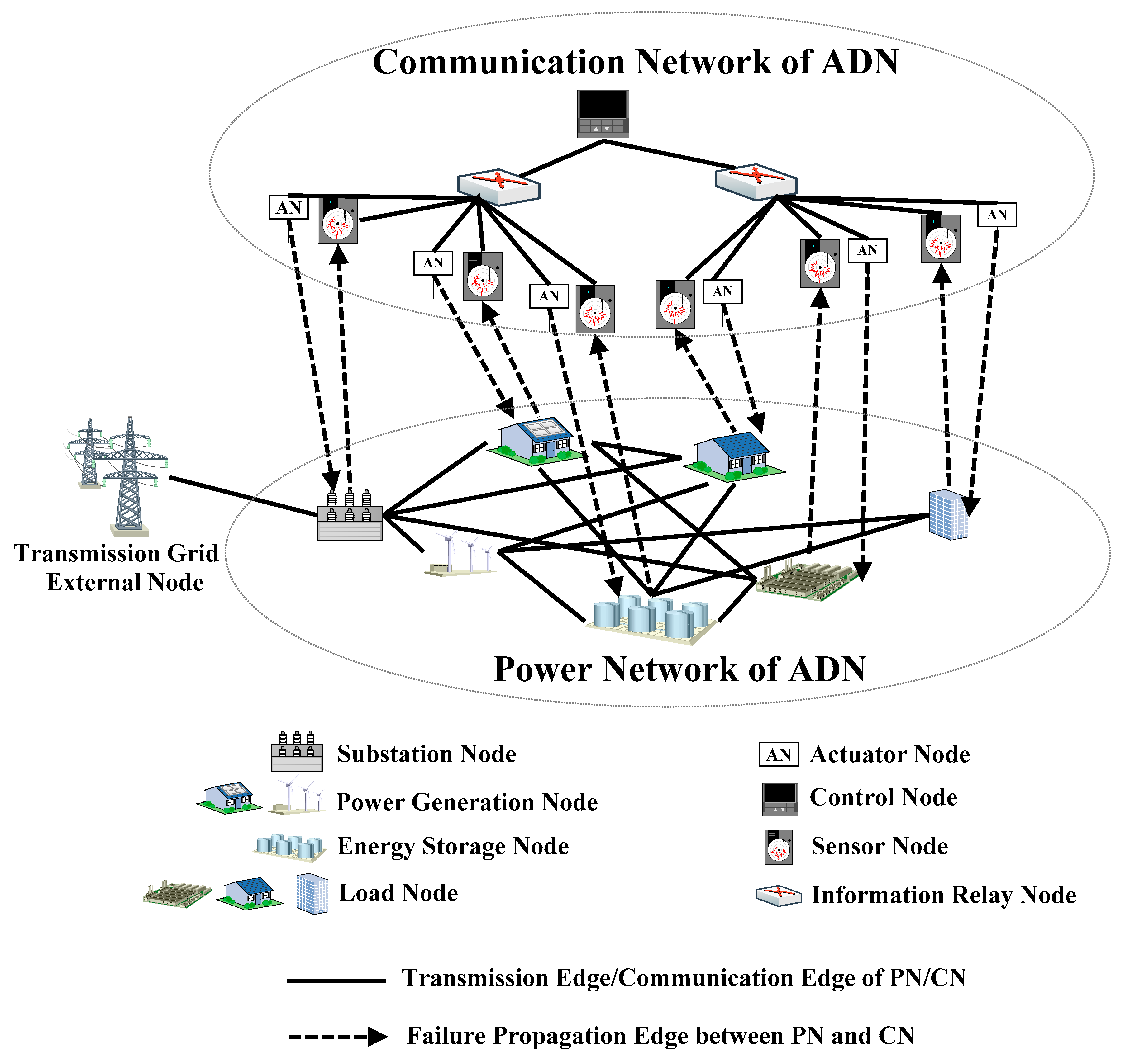
3. Active Distribution Networks Modeling

There were five types of nodes in the PN, including power generation nodes (distributed generators) VP1, substation nodes VP2, distribution nodes VP3, load nodes VP4, and external nodes (the power from transmission grid) VP5. There were four kinds of nodes in the CN, including sensor nodes VI1, information relay nodes VI2, control nodes VI3, and actuator nodes VI4. They were mutually disjoint sets.
Definition 1.
An effective control EconI in the CN refers to an effective control of the PN nodes by the control nodes of the CN, and it satisfies three conditions.
(1) 
There is at least one complete simple directed path of length k − 1 existing in the CN, that is path(nI1, nI4) = (n1, …, nk). The path has k nodes n1, …, nk. Where the source node nI1 = n1 ∈ VI1 is the sensor node, the destination node nI4 = nk ∈ VI4 is the actuator node, and at least one of the remaining nodes belongs to the VI3 nodes set. A sensor node nI1 ∈ VI1 in the CN is applied to detect failure events in the PN, and then transmit the event information to a control node nI3 ∈ VI3 through one or more information relay nodes nI2 ∈ VI2. After that, the control node nI3 ∈ VI3 generates the response information based on specific algorithms and subsequently the response information is transmitted to an actuator node nI4 ∈ VI4 through one or more information relay nodes nI2 to control the physical process.
(2) 
All nodes and edges in the path path(nI1, nI4) run normally.
(3) 
tdelay + treact < tinterval. tdelay denotes the time interval from the occurrence of a failure event to the time when the response information is generated by a node nI3. treact denotes the time interval from the time when the response information is generated to the time when the PN has been changed by actuators. tinterval denotes the minimum time interval between two adjacent failure events.
Definition 2.
The PN of the ADN is a sextuple system Gp = (VP, EP, HNP, LoadP, WP, TransP, ThresP), where
(1) 
VP represents the set of nodes in the PN, and VP = VP1 ∪ VP2 ∪ VP3 ∪ VP4 ∪ VP5.
(2) 
EP represents the edge set in the PN, and EP⊆VP × VP.
(3) 
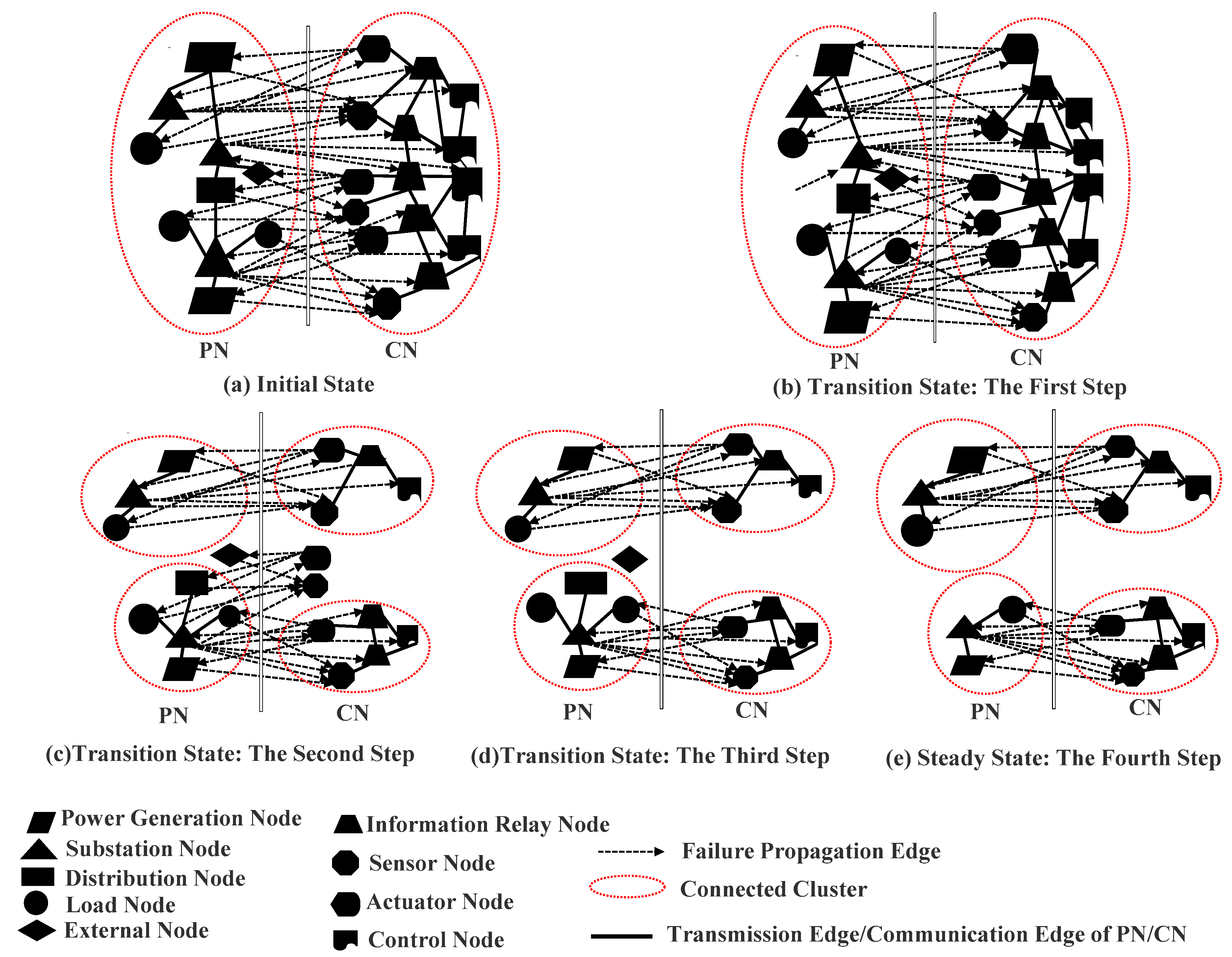
LoadP: VP×Int → C represents the load (power) of a node n in the PN at step N after the CCF occurs. Where Int represents a set of positive integer numbers, C represents the set of complex numbers. It is assumed that the load (power) of a failure node is redistributed to its neighbor node following the nearest neighbor rule. When the neighbor node nPi of a node nPj in the PN is failed, the original load (power) of this node nPi is redistributed to the node nPj, and the load (power) of this node nPj changes according to the following recursive Equation (2).
L o a d P ( n P j , N + 1 ) = { L o a d P ( n P j , N ) + L o a d P ( n P i , N ) × W P ( n P j , n P i ) n P N e i g h P ( n P i ) W P ( n P , n P i ) , n P i F a i l P L o a d P ( n P j , N ) , n P i F a i l P
where NeighP: VP→2VP is a mapping that represents the neighbor nodes set of a node in the PN. FailP is the set whose elements are the contiguous failed nodes of the node nPj, that is FailP = {nPi | nPi ∈ NeighP(nPj) ∧¬Run(nPi)}.
(4) 
WP: EP→C represents the edge weight mapping in the PN.
(5) 
TransP = (VP(N), EP(N)) represents the subgraph generated by the load (power) redistribution after a node or an edge fails in the PN at step N during the CCF. For example, if the subgraph is generated by a node nPi ∈ VP failure, then VP(N) = VP(N − 1) − OverP(NeighP(nPi)), EP(N) = EP(N − 1) − EdgP(nPi). Where OverP(NeighP(nPi)) = {n ∈ NeighP(nPi)|loadP(n,N) ≥ TPP(n)} represents the set of overloaded nodes in the set of neighbor nodes at step N. TPP(n) represents the load threshold of a node n in the PN, when the load (power) of a node n in the PN is greater than its threshold, then the node will fail. The process of an edge failure in the PN is similar.
(6) 
ThresP = ThresPJ ∪ ThresPL represents the thresholds set of nodes and edges in the PN. Where ThresPJ and ThresPL represent the thresholds sets of nodes and edges in the PN respectively. If the load flowing through an edge of the PN is greater than its threshold, then the edge will fail. The node situation is similar to the edge situation.
Since the ADN includes the PN and the CN, they are interdependent with each other. Thereinafter, the definition of the CN in the ADN is introduced, and the model of interdependence between the PN and the CN is also given.
Definition 3.
The CN of the ADN is also a sextuple system GI = (VI, EI, LoadI, WI, TransI, ThresI), where
(1) 
VI represents the set of nodes in the CN, and VI = VI1 ∪ VI2 ∪ VI3 ∪ VI4.
(2) 
EI represents the edge set in the CN, and EI⊆VI × VI.
(3) 
LoadP: VI × Int→Int represents the load (data packets) of a node n in the CN at step N after the CCF occurs. When the neighbor node nIi of a node nIj is failed, the original load (data packets) of this node nIi is redistributed to the node nIj, and the load (data packets) of the node nIj changes according to the following recursive Equation (3).
L o a d I ( n I j , N + 1 ) = { L o a d I ( n I j , N ) + L o a d I ( n I i , N ) × W I ( n I j , n I i ) n I N e i g h I ( n I i ) W I ( n I , n I i ) , n I i F a i l I L o a d I ( n I j , N ) , n I i F a i l I
where NeighI: VI→2VI is a mapping that represents the neighbor nodes set of a node in the CN. FailI is the set whose elements are the contiguous failed nodes of the node nIj, that is FailI = {nIi | nIi ∈ NeighI(nIj) ∧ ¬Run(nIi)}.
(4) 
WI: EI→Int represents the edge weight mapping in the CN.
(5) 
TransI = (VI(N), EI(N))represents the subgraph generated by the load (data packets) redistribution after a node or an edge fails in the CN at step N during the CCF.
(6) 
ThresI = ThresIN ∪ ThresIL represents the thresholds set of nodes and edges in the CN.
We modeled the interdependence between the CN and the PN in the following ways. The symbol <> represents the average value of the corresponding variable. In the CN, a sensor node nI1VI1 collects information of the nodes in the PN, and an actuator node nI4VI4 executes the commands from a control node nI3VI3 to control the physical process of the PN. Abstractly, it can be seen that a control node nK1VI3 in the CN can control K1 nodes of the PN, and the average control fan out of the node nK1 is <K1> = (1/|VI3|) × ΣK1. A node nK2 in the PN is controlled by K2 control nodes in the CN, and the average control fan in of the node nK2 is <K2> = |VI3| × <K1>/NONP. A sensor node nL1VI1 in the CN can collect L1 nodes in the PN, and the average information collecting fan in of the node nL1 is <L1> = (1/|VI1|) × ΣL1. Conversely, a node nL2 in the PN is perceived by L2 sensor nodes in the CN and the average information collecting fan out of the node nL2 is <L2> = |VI1| × <L1>/NONP. Correspondingly, the average power fan out of a node in the PN is <O2> = (1/|VP2|) × ΣO2, and a node nO1 in the CN can be power supplied by O1 nodes of the PN, then the average power fan in of the node nO1 is <O1> = |VP2| × <O2>/NONI. For example, as shown in Figure 2a, |VP1| = 2, |VP2| = 3, |VP3| = 1, |VP4| = 3, |VP5| = 1, |VI1| = 3, |VI2| = 5, |VI3| = 4, and |VI4| = 3. Therefore, <K1> = 10/4 = 2.5, <K2> = 1, <L1> = 10/3, <L2> = 1, <O1> = 1, and <O2> = 15/3 = 5. (In Appendix D, a special case about how to find <O1> and <O2> is shown)
According to the aforementioned Definitions 2 and 3, the definition of the ADN is given below.
Definition 4.
ADN is a combination of the PN and the CN, so it is also a sextuple system GA = (VA, EA, LoadA, WA, TransA, ThresA), where
(1) 
VA represents the set of nodes in the ADN, and VA = VP ∪ VI.
(2) 
EA represents the edge set in the ADN, and EA = EP ∪ EI ∪ EPI ∪ EIP. The edge set of the ADN includes the edge set of the PN and the edge set of the CN. In addition, the edge set formed by the interdependence between the nodes of the PN and CN is added. Where EPI = EPI~ ∪ EPI, it includes the virtual edge set EPI~formed by the sensor nodes in the CN perceiving the corresponding nodes in the PN, and it indicates the information gathering relationship between a sensor node nI1 ∈ VI1 in the CN and a node in the PN. The set EPI also includes the solid edge set EPI of the nodes in the PN supplying power to the nodes in the CN. EIP represents the virtual edge set formed by the actuator nodes in the CN acting on the nodes in the PN.
(3) 
LoadP: VA ×Int→C represents the load of a node n in the ADN at step N after the CCF occurs. Where Int represents a set of positive integer numbers, C represents the set of complex numbers. It is assumed that the load of a failure node is only redistributed to its neighbor node of the same network following the nearest neighbor rule.
(4) 
WA represents the edge weight mapping in the ADN, and WA: EA→C. C is a set of complex numbers.
(5) 
TransA represents a subgraph generated by the load redistribution after a node or an edge fails in the ADN at step N during the CCF, and TransA = (TransP, TransI, EPI-N, EIP-N). EPI-N represents the interdependence edges set from a node in the PN to a node in the CN. EIP-N represents the interdependence edges set from a node in the CN to a node in the PN.
(6) 
ThresA = ThresP ∪ ThresI ∪ ThresPI ∪ ThresIP represents the threshold set of nodes and edges in the ADN. ThresPI represents the threshold set of edges in the set EPI, ThresIP represents the threshold set of edges in the set EIP.
In order to analyze the robustness of the ADN against the CCF, we need to show the normal operation conditions of nodes and edges in the PN and CN respectively. The description of the relevant conditions of a normal node or an edge in the PN and CN is shown in Table 2.

4. Robustness Analysis of the ADN against the CCF

We analyzed the relationship between the robustness of the ADN and the distribution of generators, unintentional random initial failure, interdependence, network topology, and load redistribution using the percolation-based method. We reached five conclusions and the conditions that prevent the occurrence of the CCF caused by the load redistribution.

4.1. Robustness Analysis

The following analysis only considered the case of nodes failure. In this section, it was assumed that the nodes failures started from the PN.
According to the description of RP(N), fP(RP(N)), and RPF(N) in Table 1, the expected proportion of normal operational nodes after the CCF occurs at step N is RPF(N) = RP(N) × fP(RP(N)).
Furthermore, for the CN, according to the description of RI(N), fI(RI(N)), and RIF(N) in Table 1, then the expected proportion of normal operational nodes after the CCF occur at step N is RIF(N) = RI(N)*fI(RI(N)). (Where the derivation of the specific expressions of the mapping fP: RR and the mapping fI: RR are in Appendix B.)
It is assumed that the unintentional-random-initial-failure-rate is ΘP in the PN. We can get the analysis process represented by a Venn diagram, as shown in Figure 3 (The detailed analysis process is shown in Appendix C). This figure shows the process of calculating the expected proportions of normal operation nodes in the first three iterations after the CCF occurs.

4.1.1. Distribution of Generators and Robustness of the ADN

The resulting-iteration-equation-sets are concluded in (4a,b), where RI(0) =1 and RIF(0) = 1. The iteration Equation (4a) calculates the value of RP(2N + 1) using the value of RIF(2N), and the iteration Equation (4b) calculates the value of RI(2N) using the value of RPF(2N − 1). As N→∞, the iteration Equation (4a,b) calculate the sequences RI(0), RP(1), RI(2)…, RP(∞), RI(∞) and RIF(0), RPF(1), RIF(2)…, RPF(∞), RIF(∞).
{ R P ( 2 N + 1 ) = ( 1 θ P ) × [ 1 ( 1 R I F ( 2 N ) ) K 2 ] R P F ( 2 N + 1 ) = R P ( 2 N + 1 ) × f P ( R P ( 2 N + 1 ) ) , N = 0 , 1 , 2 ,
{ R I ( 2 N ) = 1 [ 1 R P F ( 2 N 1 ) ] O 1 R I F ( 2 N ) = R I ( 2 N ) × f I ( R I ( 2 N ) ) , N = 1 , 2 ,
When the CCF stops, the ADN enters the steady state and then satisfies the equations RP(2N − 1) = RP(2N) = RP(2N + 1) = λ and RI(2N − 1) = RI(2N) = RI(2N + 1) = γ. According to Equation (4a,b), a set of steady-state nonlinear equations is obtained after the replacement as above, shown in Equation (5).
{ γ = 1 [ 1 λ × f P ( λ ) ] O 1 λ = ( 1 θ P ) × [ 1 ( 1 γ f I ( γ ) ) K 2 ]
At steady state, the final expected proportions RPF(∞) and RIF(∞) of remaining normal operational nodes in the PN and CN are shown in Equation (6).
{ R P F ( ) = lim N R P F ( N ) = λ × f P ( λ ) R I F ( ) = lim N R I F ( N ) = γ × f I ( γ )
The Equations (5) and (6) are the analytical model to evaluate the robustness of the ADN against the CCF. The relationship between the final expected proportions RPF(∞) and RIF(∞) of remaining normal operational nodes and the load redistribution is embodied in the mapping fP: RR and mapping fI: RR (in Appendix B). It can be seen from the conclusion in literature [26] that in the case of distributed generators existing in the PN, fI(γ) and fP(λ) will become larger. According to Equations (5) and (6), the distribution of generators will increase the final expected proportions RPF(∞) and RIF(∞) of remaining normal operational nodes. Therefore, the first conclusion of our analysis is that the distribution of generators improves the robustness of the ADN against the CCF.

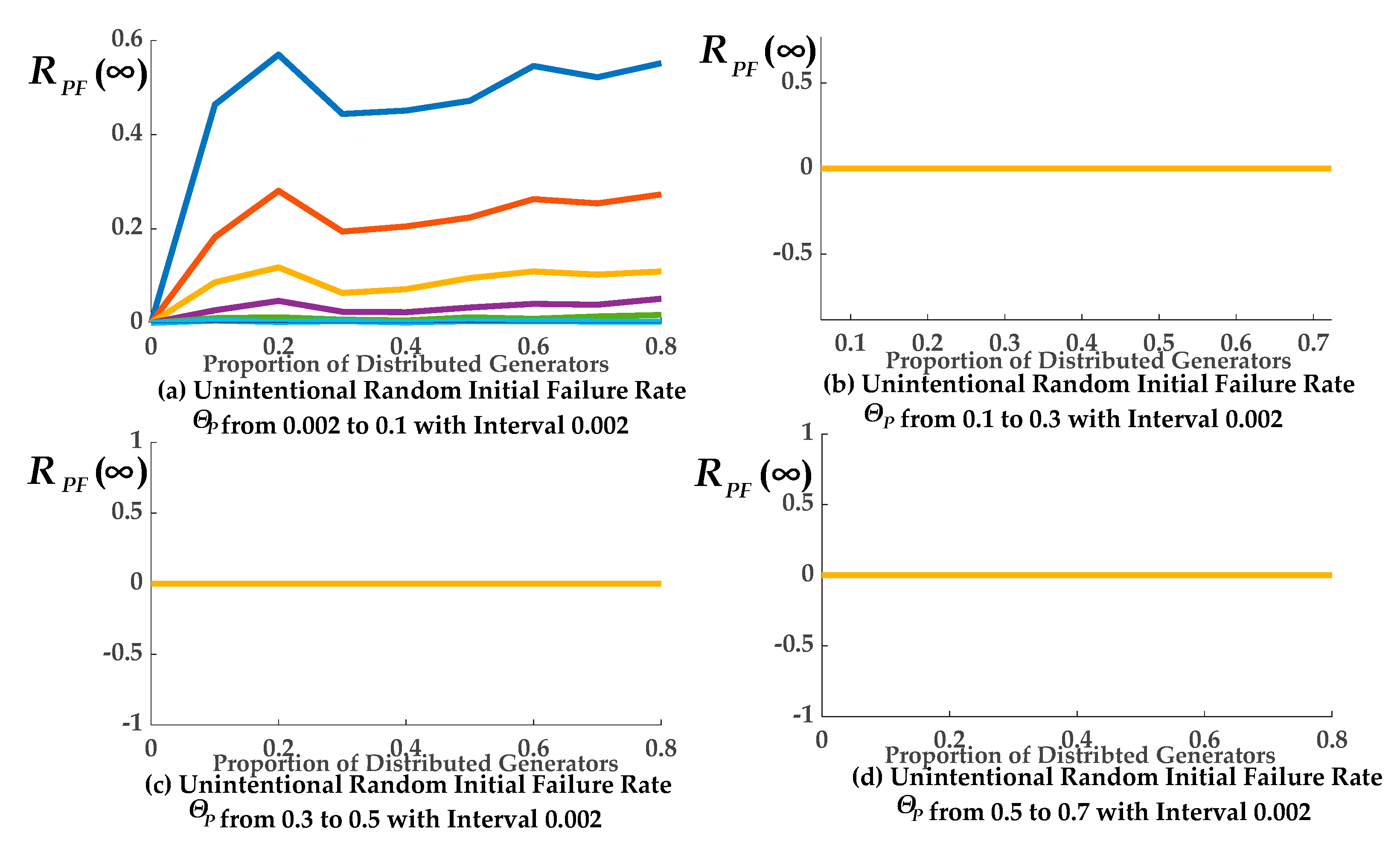
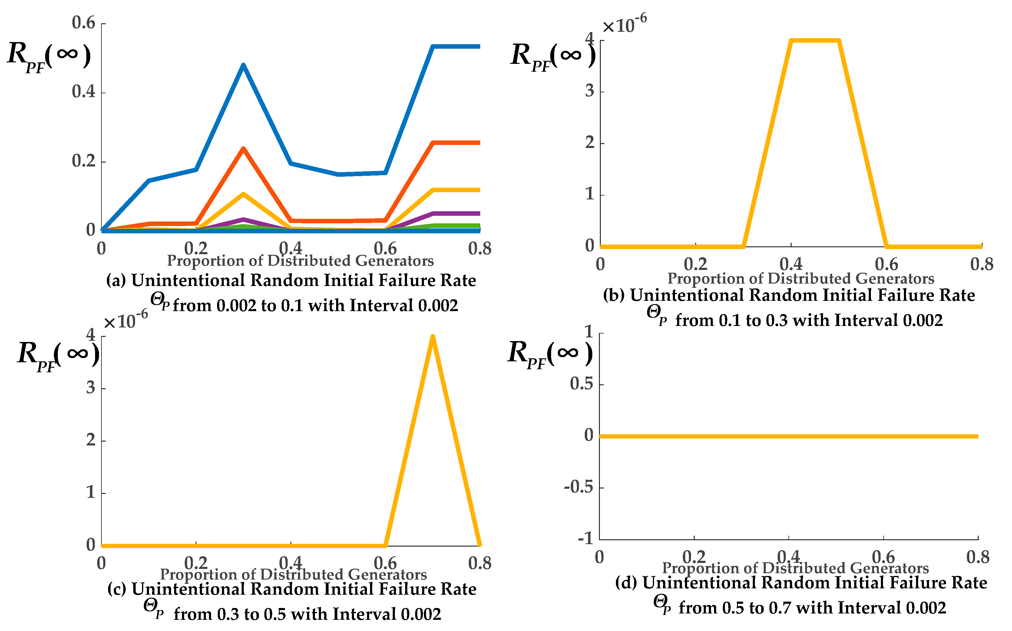
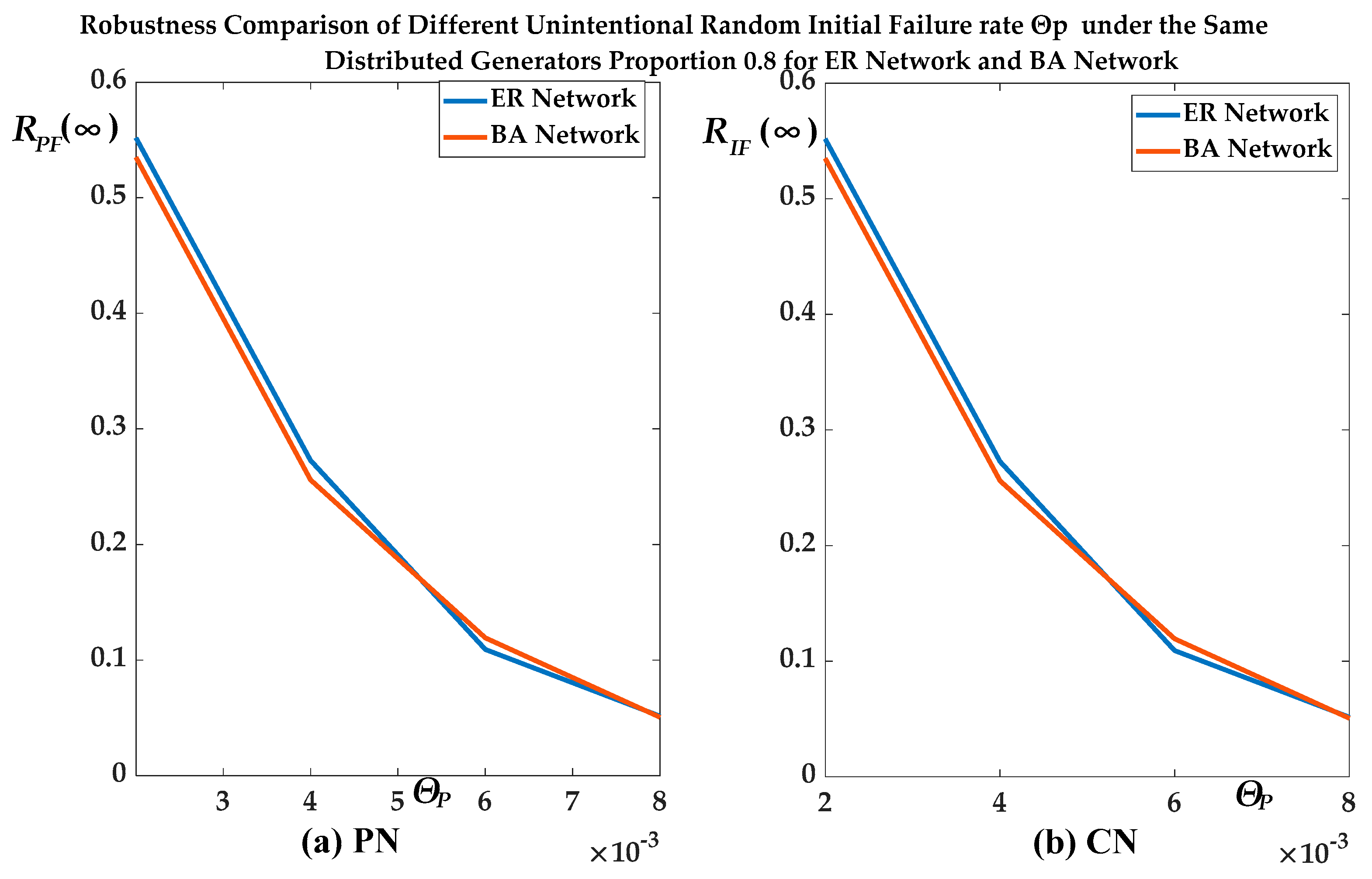
4.1.2. Unintentional Random Initial Failure Rate and Robustness of the ADN

From the Equation (5), Equation (7) can be further obtained.
γ = 1 [ 1 ( 1 θ P ) × [ 1 ( 1 γ × f I ( γ ) ) K 2 ] × f P ( ( 1 θ P ) × [ 1 ( 1 γ × f I ( γ ) ) K 2 ] ) ] O 1
The solution of Equation (7) can be obtained by the graphic method of two curves as follows in Equation (8).
{ λ = γ λ = 1 [ 1 ( 1 θ P ) × [ 1 ( 1 γ × f I ( γ ) ) K 2 ] × f P ( ( 1 θ P ) × [ 1 ( 1 γ × f I ( γ ) ) K 2 ] ) ] O 1
By solving Equation (8), we can get that it has a trivial solution γ = 0, λ = 0. That is, an intersection point of the two curves is the original point. The meaning of this trivial solution is that for any ΘP, the expected proportions RIF(∞) and RPF(∞) of normal operational nodes in the PN and CN are zero. There is another solution which corresponds to the critical value ΘP_critical of ΘP. When the two curves in Equation (8) are tangent, that is ∂λ/γ =1. We can get the equation set for solving ΘP_critical as follows in Equation (9).
{ 1 = [ 1 λ × f P ( λ ) ] O 1 1 × [ λ γ × ( f P ( λ ) + λ × f P ( λ ) γ ) ] γ = 1 [ 1 ( 1 θ P _ c r i t i c a l ) × [ 1 ( 1 γ × f I ( γ ) ) K 2 ] × f P ( ( 1 θ P _ c r i t i c a l ) × [ 1 ( 1 γ × f I ( γ ) ) K 2 ] ) ] O 1
where these equations are nonlinear and the critical value ΘP_critical of ΘP can be solved by numerical methods.
The relationship between the final expected proportions RIF(∞) and RPF(∞) of remaining normal operational nodes and the unintentional random initial failure rate ΘP is obtained by solving the nonlinear Equation (5). From Equation (5), it can be seen that the greater the unintentional random initial failure rate ΘP is, the smaller γ and λ. When the value of the unintentional random initial failure rate ΘP is greater than the critical value ΘP_critical, the solution of Equation (7) is only the trivial solution γ = 0, λ = 0. Therefore, the second conclusion of our analysis is that the robustness of the ADN is negatively correlated with the unintentional random failure rate ΘP. Once the value of ΘP is greater than the critical value ΘP_critical, the whole ADN will collapse totally.

4.1.3. Independence and Robustness of the ADN

The relationship between the final expected proportions RPF(∞) and RIF(∞) of remaining normal operational nodes and the interdependence between two sub-networks is given by the following Theorem 1.
Theorem 1.
Given network topology parameters and the unintentional random initial failure rate ΘP of a node in the PN, the robustness of a ADN is better when the value of average control fan in <K2> of a node in the PN and the value of average power fan in <O1> of a node in the CN are greater.
Proof. 
In the nonlinear Equation (5) (1 − λ × fP(λ)) < 1, when the value of average power fan in <O1> of a node in the CN is greater, the value of γ is greater. Correspondingly, given the unintentional random initial failure rate ΘP, in the nonlinear Equation (5) (1 − γ × fI(γ)) < 1, when the value of average control fan in <K2> of a node in the PN is greater, the value of λ is greater. In addition, according to the conclusion in literature [23], given network topology, fI(γ) and fP(λ) are nondecreasing functions. When the value of average control fan in <K2> of a node in the PN and the value of average power fan in <O1> of a node in the CN is greater, the final expected proportions RPF(∞) and RIF(∞) of remaining normal operational nodes in the PN and CN are greater, so the robustness of the ADN is better.
Therefore, the third conclusion of our analysis is that the robustness of the ADN is improved when the value of average control fan in <K2> of a node in the PN and the value of average power fan in <O1> of a node in the CN are greater. □

4.1.4. Network Topology and Robustness of the ADN

The relationship between the final expected proportions RPF(∞) and RIF(∞) of remaining normal operational nodes and the network topology is mainly reflected in the probability of occurrence of the event EvtP3 and the event EvtI3, then in fP(λ) and fI(γ) (in Appendix B). EvtP3 is an event which is defined to represent the failure of a node n of the PN due to the load redistribution caused by the failure of its neighbor nodes. EvtI3 is an event which represents the failure of a node n in the CN due to the load (data packets) redistribution caused by the failure of its neighbor nodes. Under the same average node degree, fP(λ) and fI(γ) of a BA network is smaller than that of an ER network (see Appendix B analysis). Therefore, the fourth conclusion of our analysis is that the robustness of the ADN with ER network topological structure is greater than that with BA network topological structure under the same average node degree.

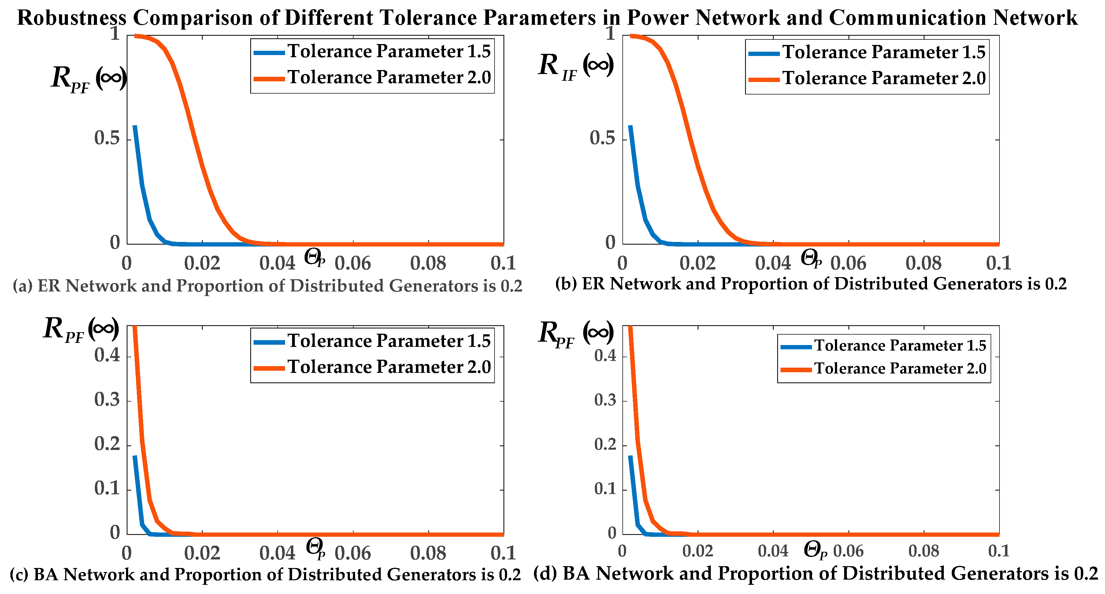
4.2. Relationship Analysis of Robustness and Tolerance Parameters

With the increase of the value of parameter reflecting the nodes thresholds under random attack strategy, the survivability of the single PN increased gradually against cascading failures, as shown in Figure 4. Therefore it was necessary to analyze the nodes thresholds influence on the robustness of the ADN. These nodes thresholds analyses provided conditions for preventing the CCF.
Assuming that the degree (it equals the sum of fan in and fan out) of a node nPi in the PN is dP. Considering the power fluctuation of the distributed generators and the initial load of the node nPi at step 0 is shown in Equation (10), which is modified from the conclusions in the literature [23].
l o a d P = d P = 1 F P ( d P ) × P r o b P ( d P ) + g
where the load FP(dP) of the node nPi in the PN is the function of its degree dP. According to the Central Limit Law, this paper used the conclusions in literature [13] to model the randomness of the output power of distributed generators. So, ξPi is a random variable obeying Gaussian distribution.
The expected load of the node nPi in the PN is shown in Equation (11).
l o a d P = d P = 1 F P ( d P ) × P r o b P ( d P ) + g
where g represents the expected output power by the distributed generators at the node nPi, if the node nPi belongs to the set of generation nodes VP1, g is not equal to zero, otherwise, it is zero. ProbP(dP) is the probability that the degree of the node nPi is dP.
The threshold of a node nPi in the PN at step N is equal to TPP(nPi,N) = αP × FP(dP). Where αP is a tolerance parameter of the node nPi and satisfies αP ≥ 1. The expected value of the threshold of the node nPi in the PN is shown in Equation (12).
T h r e s P = α P × d P = 1 F P ( d P ) × P r o b P ( d P )
Similarly, assuming that the degree of a node nIi in the CN is dI, then the initial load (data packets) of node nIi at step 0 after the CCF occur is shown in Equation (13).
L o a d I ( n I i , 0 ) = F I ( d I )
The expected load of the node nIi in the CN is shown in Equation (14).
l o a d I = d I = 1 F I ( d I ) × P r o b I ( d I )
where ProbI(dI) is the probability that the degree of the node nIi is dI.
The threshold of a node nIi in the CN is equal to TIP(nIi,N) = αI × FI(dI). Where αI is a tolerance parameter of the node nIi and satisfies αI ≥ 1. The expected value of the threshold of the node nIi in the CN is shown in Equation (15).
T h r e s I = α I × d I = 1 F I ( d I ) × P r o b I ( d P )
It is assumed that the unintentional random initial failure rate of nodes in the PN and CN are ΘP and ΘI respectively. The expected proportion of the remaining normal operational nodes in the PN is (1 − ΘP) × fP(1 − ΘP). When the node fails, the load of the original node will be redistributed to the remaining nodes in the PN, and the total redistributed load in the PN is NONP × (1 − (1 − ΘP) × fP(1 − ΘP)) × <loadP>. Correspondingly, the total redistributed load (data packets) in the CN is NONI × (1 − (1 − ΘI) × fI(1 − ΘI)) × <loadI>.
In order to avoid the subsequent nodes failure after the failure of a node, it is required that the redistributed load should not exceed the margin of the remaining nodes in the PN. After simplification, the condition is (1 − ΘP) × fP(1 − ΘP) × <ThresP> ≥ <loadP>. Accordingly, the condition in the CN is (1 − ΘI) × fI(1 − ΘI) × <ThresI> ≥ <loadI>.
Proposition  1.
When the tolerance parameters increase to infinity, that are αP→∞ and αI→∞, the expected proportions RPF(2N + 1) and RIF(2N) of the remaining normal operational nodes reach their upper limits, which are the results of a pure interdependence model without considering the load redistribution. (The proof of Proposition 1 is given in Appendix E.)
Therefore, according to Proposition 1, the fifth conclusion of our analysis is that the robustness of the ADN is greater, when the tolerance parameters increase.
If the redistributed load is equal to its margin of the remaining nodes, then the expected tolerance parameters are shown in Equations (16) and (17).
α P = d P = 1 F P ( d P ) × P r o b P ( d P ) + g θ P × f P ( θ P ) × d P = 1 F P ( d P ) × P r o b P ( d P ) = 1 + ( g d P = 1 F P ( d P ) × P r o b P ( d P ) ) θ P × f P ( θ P )
α I = d I = 1 F I ( d P ) × P r o b I ( d I ) θ I × f I ( θ I ) × d I = 1 F I ( d I ) × P r o b I ( d I ) = 1 θ I × f I ( θ I )
Furthermore, the expected critical tolerance parameters <αP-Critical> and <αI-Critical> can be obtained in Equations (18) and (19).
α P - C r i t i c a l = 1 + ( g d P = 1 F P ( d P ) × P r o b P ( d P ) ) λ × f P ( λ )
α I - C r i t i c a l = 1 γ × f I ( γ )
If the tolerance parameters αP and αI are greater than these critical ones respectively, the CCF caused by the load redistribution will not occur, which improves the robustness of the ADN against the CCF.

4.3. Evaluation Robustness

Based on the normal operation conditions of nodes and edges and the nearest neighbor rule of the load redistribution, a CCF simulation algorithm for the ADN is proposed in Algorithm 1, which is called stead-state subgraph generating algorithm. This algorithm accepts the ADN and its initial failure set, and then generates subgraphs of the ADN at steady state after the CCF stop.
Algorithm 1 Stead-state Subgraph Generating Algorithm (taking nodes failures of the PN as an example)
  Input: ADN GA = (VA, EA, LoadA, WA, TransA, ThresA). Initial failure set Vf-initialVP.
 
  // Initialization
1  t ← 0, FLP(t) ← Vf-initial, FLI(t) ← Ø, VP(t) ← VP, VI(t) ← VI;
2  whileadditional failures are possibledo
3   tt+1;
  // Load redistribution for GP and GI
4   for n ∈ (VPVI) do
5    Load redistribution according to the nearest neighbor rule;
  // Intra-network failures for GP
6   foruPVP(t) do
7    for qPVP1(t) do
8      if ((loadP(uP, t) >TPP(uP)) ∨ ( run(qP) ∧path(uP, qP) = Ø) ) then
9       FLP (t) ← FLP(t) ∪ {uP};
  // Inter-network failures for GP
10   forvPVP(t) do
11     for uIVI(t) do
12      if ((vP, uI) ∈ EPI)) ∧ (¬run(uI) ) then
13       FLP(t) ← FLP(t) ∪ {vP};
14   VP(t) ← VP(t−1) − FLP(t);
  // Intra-network failures for GI
15    for vIVI(t) do
16     for nI4VI4do
17      if (loadI(vI, t) >TIP(vI)) ∨ (path(vI,nI4) ∉Btr) then
18       FLI(t) ← FLI(t) ∪ {vI};
  // Inter-network failures for GI
19   forvIVI(t) do
20     for uPVP(t) do
21      if ((vI, uP) ∈ EIP)) ∧ (¬run(uP) ) then
22       FLI(t) ← FLI(t) ∪ {vI};
23    VI(t) ← VI(t−1) − FLI(t);
 
  Output: Sub-graphs of the ADN at steady state after the CCF stops.
After the steady state subgraphs were generated, we needed to evaluate the robustness of the ADN using Equation (1). The evaluation algorithm is proposed in Algorithm 2, which is used to evaluate the proportion of normal operational nodes in the ADN.
Algorithm 2 Evaluation Algorithm
  Input: Sub-graphs of the ADN at steady state after the CCF stops.
 
  // Initialization
1  RPF(∞) ← 0, RIF(∞) ← 0, NONP ← |VP|, NONI ← |VI|;
2  Count the number of connected clusters in Sub-graphs of the ADN, generate sets SP(Vf-initial, ∞) and SI(Vf-initial, ∞);
3  Decide generators in sets SP(Vf-initial, ∞) and SI(Vf-initial, ∞), generate sets SPg(Vf-initial, ∞) and SIg(Vf-initial, ∞);
  // Evaluate the proportion of normal operational nodes in the ADN
4  for sPSPg(Vf-initial, ∞) do
5   RPF() ← RPF() + | sP |;
6  for sISIg(Vf-initial, ∞) do
7   RIF() ← RIF() + | sI |;
8  RPF() ← RPF()/NONP;
9  RIF() ← RIF()/NONI;
 
  Output: The proportion of normal operational nodes in the ADN.
According to Equation (1), the robustness evaluation algorithm is proposed in Algorithm 3, which is used to evaluate the robustness of the ADN.
Algorithm 3 Robustness Evaluation Algorithm
  Input: Number of experiments Num.
  ADN GA = (VA, EA, LoadA, WA, TransA, ThresA).
   Initial failure set Vf-initialVP.
 
  // Initialization
1  RPF() ← 0, RIF() ← 0, countNum, NONP|VP|, NONI|VI|;
  // Evaluate the robustness of the ADN
2  whilecount0 do
3   count--;
4   SubgraphsRun the Stead-state Subgraph Generating Algorithm;
5   RPF(), RIF() ← Run the Evaluation Algorithm;
6   RPF() ← RPF()/(Num×NONP);
7   RIF() ← RIF()/(Num×NONI);
 
  Output: RPF(∞) and RIF(∞).

5. Numerical Simulations

In this section, we validate the above theoretical analysis by the data obtained from the simulation examples. We first describe the simulation experiment settings and then explain the simulation results.

5.1. Simulation Experiment Setting

An Erdos–Renyi model and a Barabasi–Albert model were used to construct a random network and a scale-free network respectively.
We designed a simulation experiment to illustrate the robustness of the ADN against the CCF in the following way. All the parameters used below are involved in the numerical simulations of References [6,7,8,15,16] except the proportion of distributed generators.
(1)
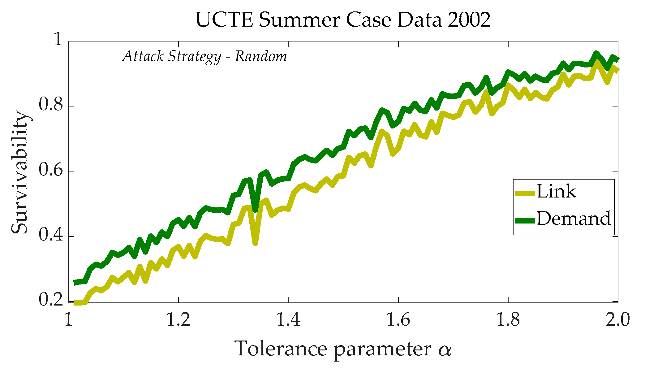
We constructed a PN and a CN respectively, and the topological structure of the PN and CN was divided into two cases: one was that the topology of the PN and CN was both scale-free, the other one was that the topology of the PN and CN was both random. There were two cases about the values of the tolerance parameters of the nodes in the PN and CN: one was both 1.5 and the other was both 2.0.
(2)
The interdependence model between the PN and CN could be divided into two situations: one was to use one-to-one interdependence model between the two networks (PN and CN), the second one was to use three-to-three interdependence model to combine the two sub-networks (PN and CN) to form a coupling network (ADN).
(3)
The unintentional random initial failure mode was to select the failure nodes in the PN randomly according to a uniform distribution.
Generators were randomly distributed with uniform distribution in the PN. The number of nodes in the PN and CN were 500 respectively and the average degree of the nodes in the PN and CN was both 5. The unintentional random failure rate ΘP was from 0.002 to 0.7 with an interval of 0.002, and there were 350 non-repetitive points in total. The proportion of distributed generators was from 0.0 to 0.8 with an interval of 0.1. A total of 74 groups were run, and there were 1000 simulation experiments in each group.

5.2. Simulation Results

After finishing the simulation experiments, we used Equation (1) to calculate the robustness indicator (RPF(∞) and RIF(∞)). Our main aim was to find the relations between the distribution of the generators, unintentional random initial failure rate, interdependence, the network topology, tolerance parameters, and the ADN robustness against the CCF. The concrete results were as follows.

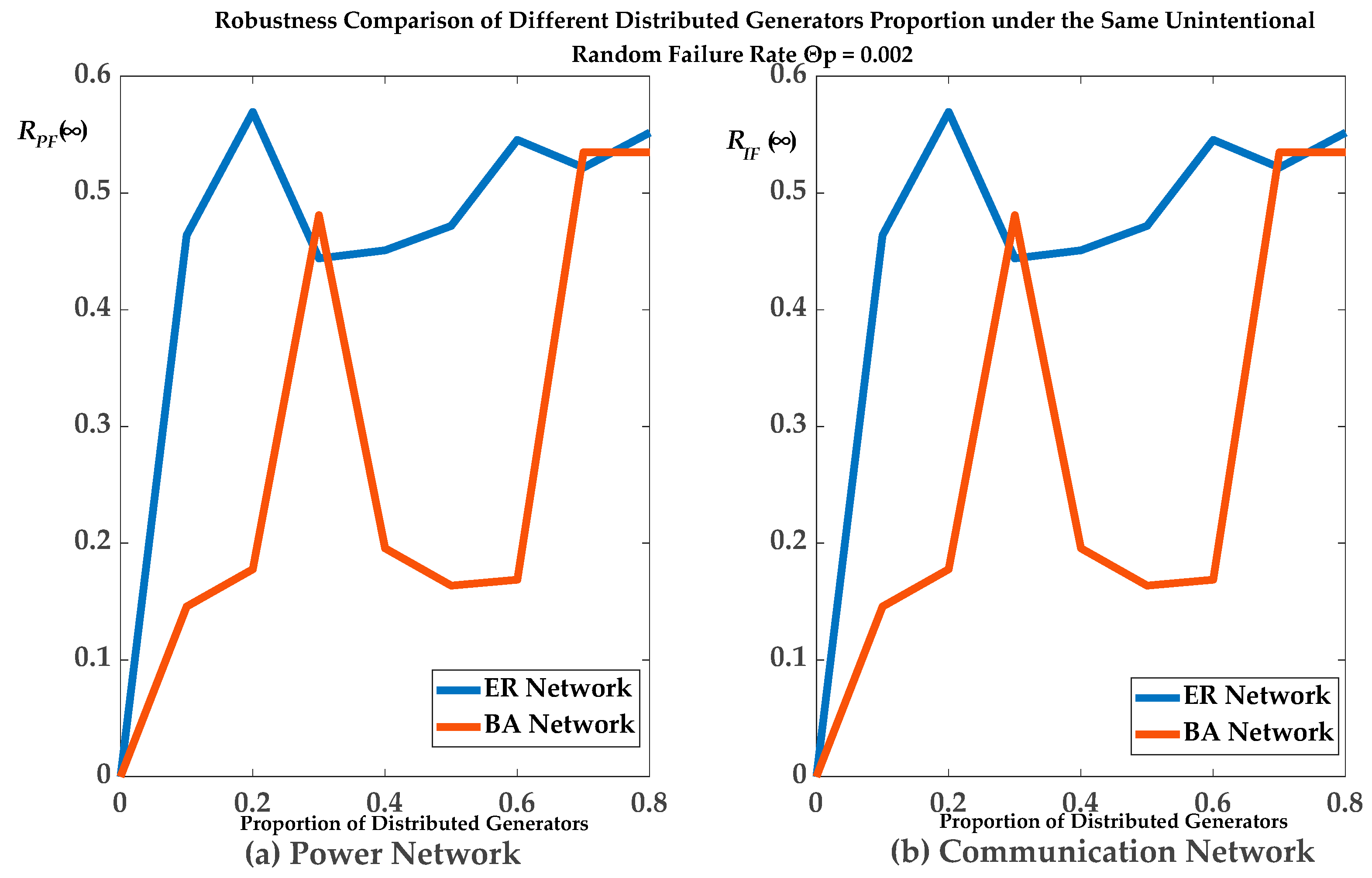
5.2.1. Distribution of Distributed Generators and Robustness

We first discuss the relationship between the distribution of distributed generators and the ADN robustness, where the unintentional random initial failure rate ΘP was from 0.002 to 0.7 with interval 0.002 and the value of the tolerance parameters of the nodes is 1.5.
The relationship between the final expected proportions RPF(∞) of the remaining normal operational nodes in the PN and the number of distributed generators (distribution of distributed generators) is shown in Figure 5 and Figure 6. In Figure 5 and Figure 6, each contains four sub-graphs respectively. In the following four sub-graphs, the first one shows 50 different curves and the rest sub-graphs show 101 different curves respectively. Each of the following eight sub-graphs show different curves representing the different unintentional random initial failure rate under the ER and BA topological structures respectively.
Of the nodes in the PN, 17.76% survived for ΘP = 0.002 with one-to-one interdependence under the ER topological structure, when the proportion of distributed generators was 0.2. Of the nodes 45.1% survived for ΘP = 0.002 with one-to-one interdependence under the ER topological structure, when the proportion of distributed generators was 0.4. Of the nodes55.17% survived in the PN for ΘP = 0.002 with one-to-one interdependence under the ER topological structure, when the proportion of distributed generators was 0.8.
As shown in Figure 5a and Figure 6a, RPF(∞) fluctuated with the proportion of distributed generators due to the uncertainty of the CCF, and they were positively correlated as a whole. Therefore, this agreed with our first conclusion. That is, the robustness of the ADN was improved when the number of distributed generators was greater.
In the other sub-graphs, ΘP is too high, which led to the whole network crashing, thus making RPF(∞) almost equal to zero. The relationship between the final expected proportions RIF(∞) of the remaining normal operational nodes in the CN and the number of distributed generators was similar.

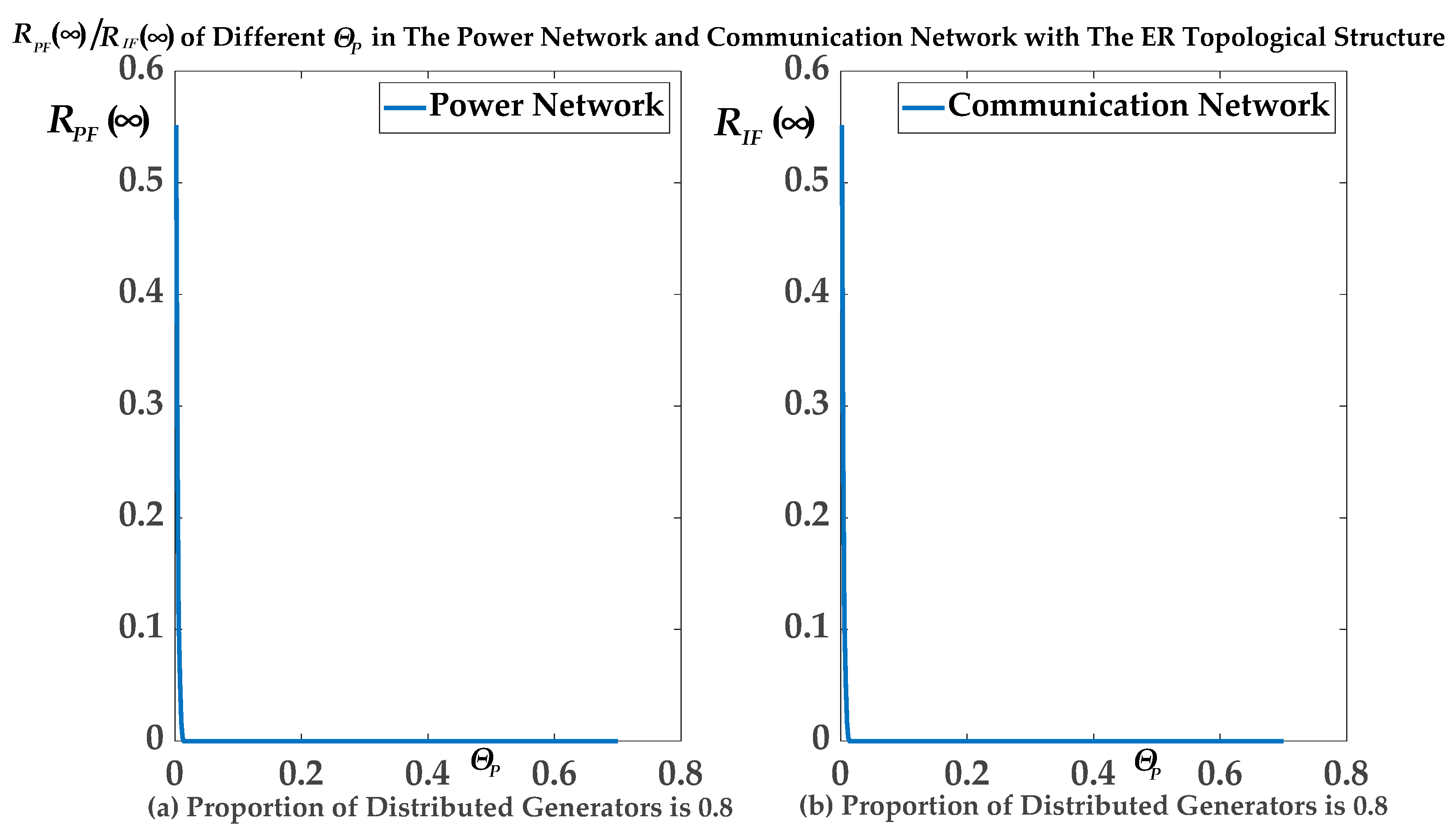
5.2.2. ΘP and Robustness

We then investigated the relationship between the unintentional random initial failure rate ΘP and the ADN robustness under the ER topological structure, where the proportion of distributed generators was 0.8 and the value of the tolerance parameters of the nodes was 1.5.
Figure 7 clearly shows the relationship between the final expected proportions RPF(∞)/RIF(∞) of the remaining normal operational nodes in the PN/CN and the unintentional random initial failure rate ΘP. Of the nodes in the PN, 55.17% survived for ΘP = 0.002 when the proportion of distributed generators was 0.8 under the ER topological structure. Of nodes in the PN, 27.27% survived for ΘP = 0.004 when the proportion of distributed generators was 0.8 under the ER topological structure. Accordingly, 55.17% of nodes in the CN survived for ΘP = 0.002 when the proportion of distributed generators was 0.8 under the ER topological structure. Of nodes in the CN, 27.27% survived for ΘP = 0.004 when the proportion of distributed generators was 0.8 under the ER topological structure.
As shown in Figure 7, it can be seen that the robustness of the ADN deteriorated when the unintentional random initial failure rate ΘP in the PN was greater. That is, the more the unintentional random failure rate was, the robustness of ADN against the CCF was worse. We also observed that the transition phase of RPF(∞) was very sharp, and this indicated that the PN and CN either collapsed or was whole totally. Therefore, this agreed with our second conclusion. That is, the robustness of the ADN was negatively correlated with the unintentional random failure rate ΘP. Once the value of ΘP was greater than the critical value ΘP_critical, the whole ADN collapsed totally.
The relationship between the final expected proportions RIF(∞) of remaining normal operational nodes in the CN and the unintentional random initial failure rate ΘP is similar.

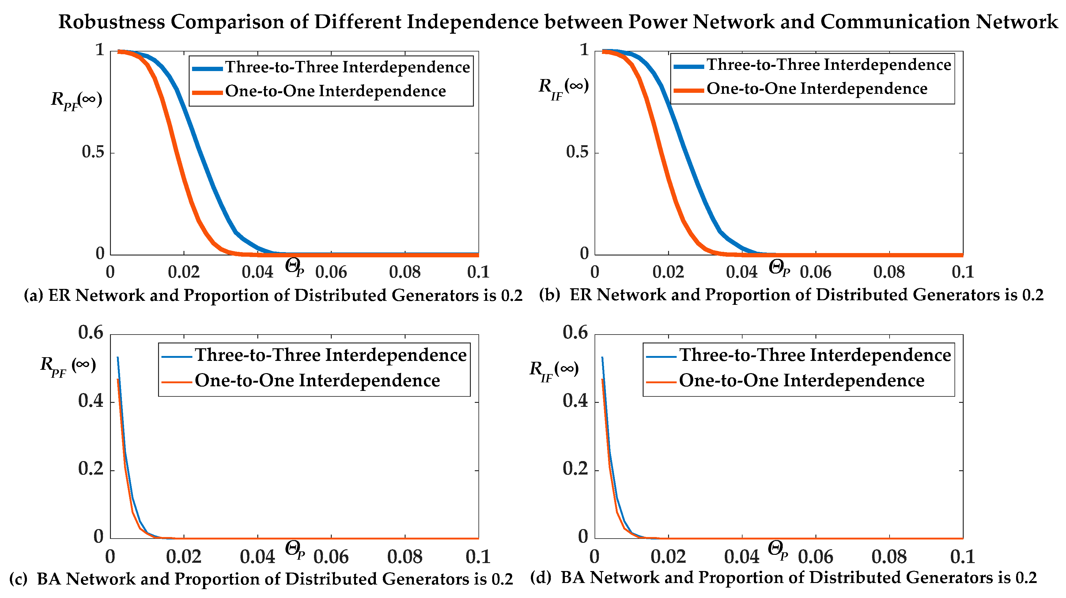
5.2.3. Independence and Robustness

We then investigated the relationship between the interdependence and the ADN robustness under the ER/BA topological structure, which is shown in Figure 8, where the proportion of distributed generators was 0.2 and the value of the tolerance parameters of the nodes was 1.5. One-to-one interdependence represented <K2> = 1, and <O1> = 1; three-to-three Interdependence represented <K2> = 3, and <O1> = 3.
Of the nodes in the PN, 26.01% survived for ΘP = 0.022 with one-to-one interdependence under the ER topological structure and 62.49% of nodes in the PN survived for ΘP = 0.022 with three-to-three interdependence under the ER topological structure. Of the nodes in the CN, 26.01% survived for ΘP = 0.022 with one-to-one interdependence under the ER topological structure and 64.13% of nodes in the CN survived for ΘP = 0.022 with three-to-three interdependence under the ER topological structure. Accordingly, 21.02% of nodes in the PN survived for ΘP = 0.004 with one-to-one interdependence under the BA topological structure and 25.6% of nodes in the PN survived for ΘP = 0.004 with three-to-three interdependence under the BA topological structure. Of the nodes in the CN, 21.02% survived for ΘP = 0.004 with one-to-one interdependence under the BA topological structure and 25.6% of nodes in the CN survived for ΘP = 0.004 with three-to-three interdependence under the BA topological structure.
As shown in Figure 8, we observed that RIF(∞) and RPF(∞) of three-to-three interdependence were greater than that of one-to-one interdependence both in the ER topology and in the BA topology structure. This agreed with our third conclusion. That is, the robustness of the ADN was improved when the value of average control fan in <K2> of a node in the PN and the value of average power fan in <O1> of a node in the CN were greater.

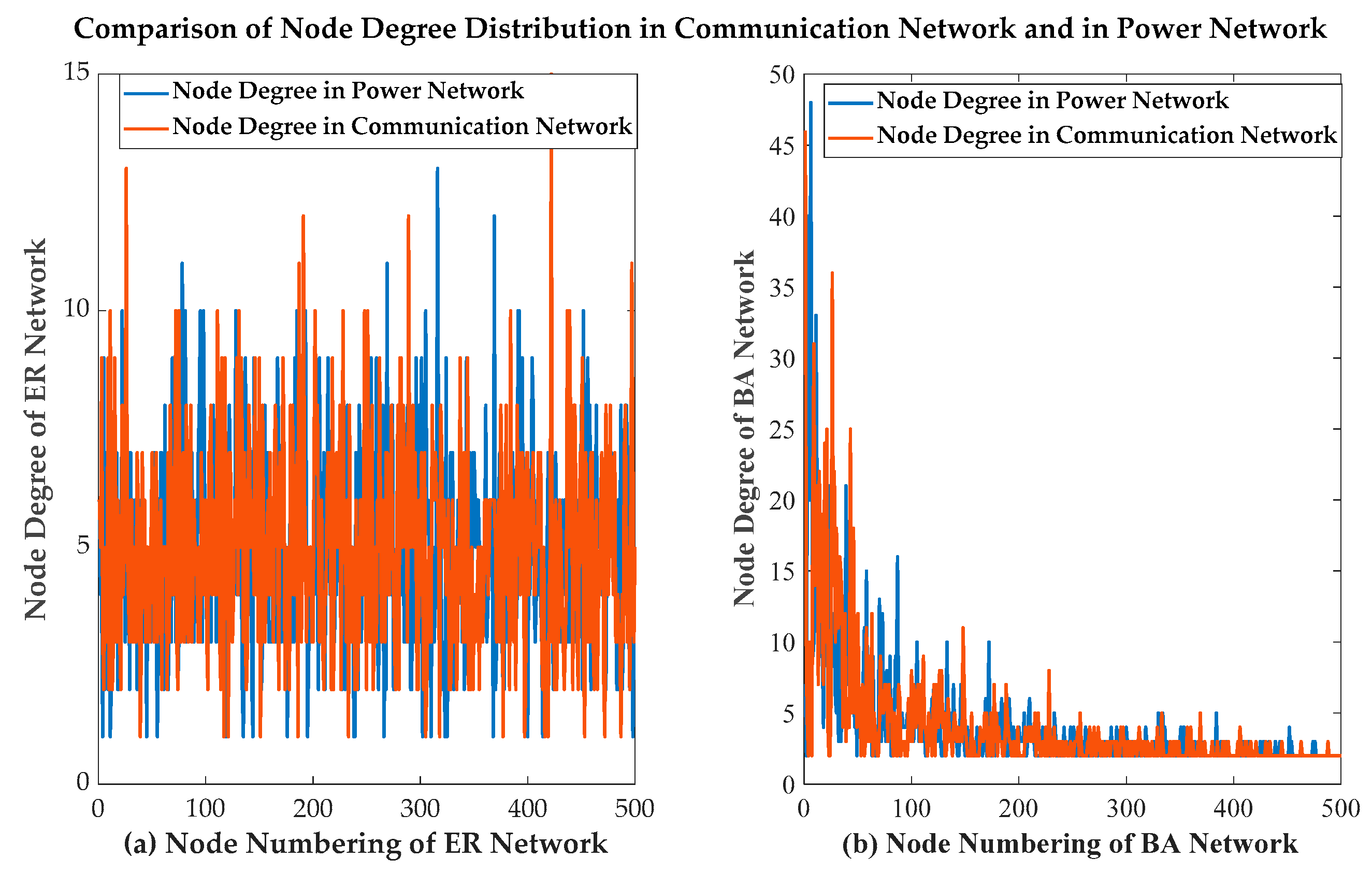
5.2.4. Network Topology and Robustness

Generally, the robustness of the ADN against the CCF was affected by the different topological structure. In Figure 9, the left side shows the node degree distribution comparison diagram when the PN and CN adopted the ER network topological structure, while the right side shows the degree comparison diagram when the BA network topological structure was adopted. We observed from Figure 9 that the degree distribution of the ER network was more uniform than the BA network. The degree distribution of the BA network followed the power law. The average degree of the ER and BA network was 5 and 5 respectively for comparison.
The relationship between the final expected proportions RPF(∞) of remaining normal operational nodes in the PN and network topology is shown in Figure 10 and Figure 11. In Figure 10, the interval of the proportion of distributed generators was from 0.0 to 0.8. Of the nodes, 54.57% survived in the PN when the proportion of distributed generators was 0.6 with unintentional random initial failure rate ΘP = 0.002 under the ER topological structure and 16.87% of nodes survived in the PN when the proportion of distributed generators was 0.6 with unintentional random initial failure rate ΘP = 0.002 under the BA topological structure. Of the nodes, 54.57% survived in the CN when the proportion of distributed generators was 0.6 with unintentional random initial failure rate ΘP = 0.002 under the ER topological structure and 16.87% of nodes survived in the CN when the proportion of distributed generators was 0.6 with unintentional random initial failure rate ΘP = 0.002 under the BA topological structure. In Figure 11, the interval of unintentional random initial failure rate ΘP is from 0.002 to 0.008. Of the nodes, 27.27% survived in the PN for ΘP = 0.004 when the proportion of distributed generators was 0.8 under the ER topological structure and 25.6% of nodes survived in the PN for ΘP = 0.004 when the proportion of distributed generators was 0.8 under the BA topological structure. Of the nodes, 27.27% survived in the CN for ΘP = 0.004 when the proportion of distributed generators was 0.8 under the ER topological structure and 25.6% of nodes survived in the CN for ΘP = 0.004 when the proportion of distributed generators was 0.8 under the BA topological structure.
As shown in Figure 10 and Figure 11, the RPF(∞) of the ER network intersected with that of BA network due to the uncertainty of the CCF, and the RPF(∞) and RIF(∞) of the ER network were greater than that of BA network as a whole. Therefore, this agreed with our fourth conclusion. That is, the robustness of the ADN with ER network topological structure was greater than that with BA network topological structure under the same average node degree.

5.2.5. Tolerance Parameters and Robustness

We investigated the relationship between the tolerance parameters and the ADN robustness when the proportion of distributed generators was 0.2.
The relationship between the final expected proportions RPF(∞) and RIF(∞) of remaining normal operational nodes and the tolerance parameters αP and αI is shown in Figure 12. Of the nodes, 1.188% survived in the PN for ΘP = 0.01 with the tolerance parameters αP = αI = 1.5 under the ER topological structure. Of the nodes, 93.37% survived in the PN for ΘP = 0.01 with the tolerance parameters αP = αI = 2.0 under the ER topological structure. Of the nodes, 1.188% survived in CN for ΘP = 0.01 with the tolerance parameters αP = αI = 1.5 under the ER topological structure and 93.37% of nodes survived in the CN for ΘP = 0.01 with the tolerance parameters αP = αI = 2.0 under the ER topological structure. Accordingly, 0% of nodes survived in the PN for ΘP = 0.01 with the tolerance parameters αP = αI = 1.5 under the BA topological structure and 1.386% of nodes survived in the PN for ΘP = 0.01 with the tolerance parameters αP = αI = 2.0 under the BA topological structure. None of the nodes survived in the CN for ΘP = 0.01 with the tolerance parameters αP = αI = 1.5 under the BA topological structure and 1.386% of nodes survived in the CN for ΘP = 0.01 with the tolerance parameters αP = αI = 2.0 under the BA topological structure.
As shown in Figure 12, RPF(∞) and RIF(∞) with the tolerance parameter 2.0 were greater than that of the tolerance parameter 1.5. Therefore, this agreed with our fifth conclusion. That is, the robustness of the ADN was positively correlated with the tolerance parameters. The robustness of the ADN was improved when the values of the nodes tolerance parameters αP in the PN and αI in the CN were greater. This also shows that the larger the tolerance parameters, the smaller the impact of load redistribution on the robustness of the ADN.

6. Related Work

Earlier studies mainly focused on the electrical power system. Research on the cascading failures of the electrical power system has a long history. Over the past two decades, the research on cascading failure propagation modes in the electrical power system has focused on two aspects: one is the single network cascading failure propagation modes [9,11,13,28] and the other is the interdependent cascading failure modes between a PN and a CN [16,22,23]. The theories for analyzing cascading failures of large blackouts include self-organization theory [28], percolation theory [15,17,21], power flow model [14,22,24], and so on.
Research on cascading failures in a single network, including random failure modes, with single or multiple nodes removal, the following problems are specifically solved: (1) The impacts exerted on cascading failures are analyzed when the power overloads lead to nodes or edges failures [11]. (2) Considering the intermittent and random nature of new energy generation, the impacts exerted on the cascading failures are analyzed in a single PN [9,11,13].
Research on the CCF of interdependent networks between a PN and a CN includes: (1) The characteristics of the CCF across the PN and CN are summarized: (a) The accidents caused by the CCF have the characteristics of power law distribution [6], and the probability distribution of large-scale blackouts caused by the increasing load or unbalanced power flow changes from the exponential tail to the power law tail. (b) Total demand or pressure leads to the operation of the interdependent network under extreme conditions, which is one of the main factors leading to the CCF. (2) After analyzing the CCF propagation mechanisms of different kinds of networks, the conclusions are as follows: (a) Scale-free networks for a single network are robust to random attacks, but two interdependent scale-free networks are sensitive to random attacks [24]. (b) Even if the small disturbances in one network can lead to failures in another network, many clusters can be isolated from the whole network after the CCF stops [15,17,21,23]. (c) From the security point of view, an interaction model is established for the importance of the coupling relationship between a PN and a supervisory control and data acquisition (SCADA) system. (d) A model has been established to analyze the process of cascading failure propagation between the PN and the CN [8,19,21,25]. Its basic idea is to calculate the power flow redistribution after cascading failures occur by the dynamic power flow. (e) A topological model of a CN and a PN is established by the graph theory, and their transmission characteristics are analyzed. The ability of different topologies to resist the CCF under different coupling conditions is analyzed and compared [20,24].
However, the above current research work does not comprehensively consider the impact of the distribution of distributed generators, network topology, interdependence, and load redistribution on the robustness of the ADN against the CCF.

7. Conclusions and Future Work

In this paper, we analyzed the relationship between the final expected proportion of remaining normal operational nodes and distribution of generators, unintentional random initial failure, interdependence, network topology, and load redistribution. We gave a CCF simulation algorithm and a robustness evaluation algorithm. The robustness of the ADN against the CCF was simulated based on the ER network topological structure and the BA network topological structure. The model analysis and the simulation analysis showed that given the specific network topology parameters and the unintentional random initial failure rate, the more the average control fan in of a node in the PN and the more the average power fan in of a node in the CN, the better the robustness of the ADN, the distribution of generators improved the robustness of the ADN against the CCF. In addition, the robustness of the ADN was improved when the values of the nodes tolerance parameters were greater. Compared with the traditional power distribution network, because of the physical distribution of generators, the CCF caused by the interdependence between the PN and CN were more difficult to occur.
This work is helpful in understanding the CCF in the ADN. Based on our above analysis on numerical simulation results, if we want to improve the robustness of the ADN against the CCF, we should take the following measures: using the more uniform degree distribution of the ADN network topology, improving the values of <O1> and <K2>, improving the number of distributed generators, improving the tolerance parameters of the nodes in the ADN and protecting the nodes from the random failures. In practice, the PN and CN of the ADN are non-linear and the topological structure of the network is asymmetric due to natural and artificial factors. Considering the effect of factors of non-linear and asymmetry on the robustness of the ADN is one of our future directions. Accordingly, making preventive control measures for the CCF in the ADN is also one of our future directions.

Author Contributions

Conceptualization, P.S. and Y.D.; methodology, P.S. and Y.D.; software, C.W. and C.L.; validation, P.S., Y.D., C.W., C.L., and K.Y.W.; formal analysis, P.S.; investigation, P.S. and Y.D.; resources, P.S., C.L., and Y.D.; data curation, P.S.; writing—original draft preparation, P.S.; writing—review and editing, P.S., Y.D., and K.Y.W.; visualization, P.S. and K.Y.W.; supervision, Y.D. and P.S.; project administration, P.S.; funding acquisition, Y.D.; All of the authors approved the final version of the manuscript.

Funding

This work was supported by the National Key Research and Development Program of China (Basic Research Class) under Grant No. 2017YFB0903000—Basic Theories and Methods of Analysis and Control of the Cyber–Physical Systems for Power Grid.

Conflicts of Interest

The authors declare no conflict of interest.

Appendix A. Symbolic Descriptions Used in Appendix

Table A1. Symbolic Descriptions used in Appendix A, Appendix B, Appendix C and Appendix D.
SymbolDescription
DP1A random variable representing the number of neighbor nodes of a node in the PN of the ADN.
DP2A random variable representing the number of nodes in neighbor nodes set (excluding the dependent nodes in the CN) NeighP(n) of a node n in the PN that can cause the node n to fail through load redistribution.
DI1A random variable representing the number of neighbor nodes of a node in the CN of the ADN.
DI2A random variable representing the number of nodes in the neighbor nodes set (excluding the dependent nodes in the PN) NeighI(n) of a node n in the CN that can cause the node n to fail through data traffic redistribution.
dPNode degree in the PN of the ADN.
dINode degree in the CN of the ADN.
EvtP1An event represents a particular neighbor node (not the dependent nodes in the CN) of a node n in the PN of the cyber–physical distribution network.
EvtP2An event where a particular node connects to the connected clusters containing generators in the PN of the ADN.
EvtP4An event represents a node with a degree dP belonging to the connected clusters containing generators in the PN of the ADN.
EvtI1An event represents a particular neighbor node (not the dependent nodes in the PN) of a node n in the CN of the ADN.
EvtI2An event where a particular node connects to the connected clusters in the CN depending on the connected clusters containing generators in the PN of the ADN.
EvtI4An event that a node in the CN with a degree dI belongs to the connected clusters depending on the connected clusters containing generators in the PN of the ADN.

Appendix B. Derivation of Mapping fP and fI

Firstly, it is assumed the degree of the node nPi is dP, and the number of neighbor nodes set NeighP(nPi) of a node nPi in the PN of the ADN is DP1 = dPO2. In order to calculate the conditional probabilities ProbP(EvtP3/|NeighP(nPi)|), then the probability needed is shown in Equation (A1).
P r o b P ( E v t P 3 D P 2 = d P ) = P r o b P ( d P × ( d P = 1 ( F P ( d P ) + g ) × W P ( n P j , n P i ) n P N e i g h P ( n P i ) W P ( n P , n P i ) × P r o b P ( d P ) ) + F P ( d P ) + ξ i > α P × F P ( d P ) )
where ( d P = 1 ( F P ( d P ) + g ) × W P ( n P j , n P i ) n P N e i g h P ( n P i ) W P ( n P , n P i ) × P r o b P ( d P ) ) is the expected load redistributed to the node nPi after the failure of a neighbor node nPj connected to the node nPi, and then there is Equation (A2).
P r o b P ( E v t P 3 D P 2 = d P ) = { 1 , d P > ( α P 1 ) × F P ( d P ) ξ i ( d P = 1 ( F P ( d P ) + g ) × W P ( n P j , n P i ) n P N e i g h P ( n P i ) W P ( n P , n P i ) × P r o b P ( d P ) ) 0 , other .
The probability of selecting d′P nodes from the neighbors set NeighP(nPi) of the node nPi in the PN is shown in Equation (A3).
P r o b P ( D P 2 = d P D P 1 = d P O 2 ) = ( d P O 2 d P ) 2 d P O 2 ,
where
2 d P O 2 = ( ( d P O 2 0 ) + ( d P O 2 1 ) + + ( d P O 2 d P O 2 ) ) .
Therefore, under the condition of the number of neighbor nodes of a node nPi is DP1 = dPO2, the probability of an event EvtP3 occurrence is shown in Equation (A5).
P r o b P ( E v t P 3 D P 1 = d P O 2 ) = d P = 0 d P O 2 P r o b P ( E v t P 3 D P 2 = d P ) × P r o b P ( D P 2 = d P D P 1 = d P O 2 ) .
After simplification, it is obtained in Equation (A6).
P r o b P ( E v t P 3 D P 1 = d P O 2 ) = 1 2 d P O 2 d P = ( α P 1 ) × F P ( d P ) ξ i ( d P = 1 ( F P ( d P ) + g ) × W P ( n P j , n P i ) n P N e i g h P ( n P i ) W P ( n P , n P i ) × P r o b P ( d P ) ) d P O 2 ( d P O 2 d P ) .
The following analysis is simplified by referring to the idea of percolation theory. A node nPi in the PN does not belong to the connected clusters with distributed generators belonging to one of the following four situations:
(1)
This node nPi has been removed due to random failures, including power fluctuations (intermittent or random) of distributed generators, etc.
(2)
This node nPi exists but does not belong to the connected clusters containing generators. It belongs to a small connected component containing no generators.
(3)
This node nPi is removed due to overload.
(4)
This node nPi is removed due to the failure of the node in the CN associated with the node nPi.
In Case (1), the probability is ΘP. In Case (2), the probability is shown in Equation (A7).
( 1 θ P ) × P r o b P ( E v t P 2 E v t P 1 ) d P O 2 .
The probability in the third case is shown in Equation (A8).
P r o b P ( E v t P 3 D P 1 = d P O 2 ) .
In the fourth case, the probability is considered in Section 4.1. In summary, the probability that a node nPi with the node failure probability ΘP belongs to the connected clusters containing generators is shown in Equation (A9).
P r o b P ( E v t P 4 ) = 1 ( θ P + ( 1 θ P ) × ( P r o b P ( E v t P 2 E v t P 1 ) d P O 2 + ( 1 P r o b P ( E v t P 2 E v t P 1 ) d P O 2 ) × P r o b P ( E v t P 3 D P 1 = d P O 2 ) ) ) .
After simplification, it is obtained in Equation (A10).
P r o b P ( E v t P 4 ) = ( 1 θ P ) × ( 1 P r o b P ( E v t P 2 E v t P 1 ) d P O 2 ) × ( 1 P r o b P ( E v t P 3 D P 1 = d P O 2 ) ) .
Thus, the expected probability that any node belongs to the connected clusters containing generators is shown in Equation (A11).
d P = max { 0 , O 2 } P r o b P ( d P ) × P r o b P ( E v t P 4 ) .
Therefore, considering the power fluctuations (intermittent or random) of distributed generators, it is defined fP(1 − ΘP) as the expected probability of the connected clusters containing generators divided by 1 − ΘP, then it is as shown in Equation (A12).
f P ( 1 θ P ) = d P = max { 0 , O 2 } P r o b P ( d P ) × P r o b P ( E v t P 4 ) 1 θ P .
The above formula is further equal to Equation (A13).
f P ( 1 θ P ) = d P = max { 0 , O 2 } P r o b P ( d P ) × ( 1 P r o b P ( E v t P 2 E v t P 1 ) d P O 2 ) × ( 1 P r o b P ( E v t P 3 D P 1 = d P O 2 ) ) .
In addition, ProbP(Evt′P2/EvtP1) is the probability that there is a particular neighbor node nP of a node nPi, and this node nP is not connected to the connected clusters containing generators in subsequent neighbor nodes except this node nPi. Thus, the conclusion is drawn as shown in Equation (A14).
P r o b P ( E v t P 2 E v t P 1 ) = 1 d P d P = 0 [ ( d P + 1 ) × P r o b P ( d P + 1 ) ] × ( 1 P r o b P ( E v t P 4 ) ) .
Secondly, the number of neighbor nodes of a node nIi in the CN of the ADN is DI1 = dIO1. In order to calculate the conditional probability ProbI(EvtI3/|NeighI(nIi)|), we need to know the conditional probability ProbI(EvtI3/DI2 = d′I) which is equal to Equation (A15).
P r o b I ( E v t I 3 D I 2 = d I ) = P r o b I ( d I × ( d = 1 F I ( d ) × W I ( n I j , n I i ) n I N e i g h I ( n I i ) W I ( n I , n I i ) × P r o b I ( d ) ) + F I ( d I ) > α I × F I ( d I ) ) ,
where d = 1 F I ( d ) × W I ( n I j , n I i ) n I N e i g h I ( n I i ) W I ( n I , n I i ) × P r o b I ( d ) is the expected data traffic flow redistributed to the node nIi after the failure of the neighbor node nIj connected to the node nIi. Then there is Equation (A16).
P r o b I ( E v t I 3 D I 2 = d I ) = { 1 , d I > ( α I 1 ) × F I ( d I ) d = 1 F I ( d ) × W I ( n I j , n I i ) n I N e i g h I ( n I i ) W I ( n I , n I i ) × P r o b I ( d ) 0 , other .
The probability of selecting a node from the neighbor nodes set NeighI(nIi) of the node nIi in the CN is shown in Equation (A17).
Pr o b I ( D I 2 = d I D I 1 = d I O 1 ) = ( d I O 1 d I ) 2 d I O 1 ,
where
2 d I O 1 = ( ( d I O 1 0 ) + ( d I O 1 1 ) + + ( d I O 1 d I O 1 ) ) .
Therefore, under the condition that the number of neighbor nodes set is DI1 = dIO1, the probability of an event EvtI3 occurring is shown in Equation (A19).
P r o b I ( E v t I 3 D I 1 = d I O 1 ) = d = 0 d I O 1 P r o b I ( E v t I 3 D I 2 = d ) × P r o b I ( D I 2 = d D I 1 = d I O 1 ) .
After further simplifications, the results are obtained as shown in Equation (A20).
P r o b I ( E v t I 3 D I 1 = d I O 1 ) = 1 2 d I O 1 d I = ( α I 1 ) × F I ( d I ) d = 1 F I ( d ) × W I ( n I j , n I i ) n I N e i g h I ( n I i ) W I ( n I , n I i ) × P r o b I ( d ) d I O 1 ( d I O 1 d I ) .
Furthermore, it is assumed that NONI × ΘI nodes fail in the CN. A node nIi does not belong to the connected clusters depending on the connected clusters containing generators in the PN due to the following four situations:
(1)
This node nIi has been removed due to random failures, etc.
(2)
This node nIi exists but does not belong to the connected clusters depending on the connected clusters containing generators in the PN.
(3)
This node nIi has been removed due to the excessive data traffic flow.
(4)
This node nIi fails due to the failure of its depending node in the PN.
The probability in Case (1) is ΘI. In Case (2), the probability is shown in Equation (A21).
( 1 θ I ) × P r o b I ( E v t I 2 E v t I 1 ) d I O 1 .
In Case (3), the probability is shown in Equation (A22).
P r o b I ( E v t I 3 D I 1 = d I O 1 ) .
In summary, the probability that a node nIi with a degree dI belongs to the connected clusters depending on the connected clusters containing generators in the PN under the node failure probability ΘI is shown in Equation (A23).
P r o b I ( E v t I 4 ) = 1 ( θ I + ( 1 θ I ) × ( P r o b I ( E v t I 2 E v t I 1 ) d I O 1 + ( 1 P r o b I ( E v t I 2 E v t I 1 ) d I O 1 ) × P r o b I ( E v t I 3 D I 1 = d I O 1 ) ) + 1 O 1 × ( 1 f P ( θ P ) ) ) .
After further simplifications, the results are obtained as shown in Equation (A24).
P r o b I ( E v t I 4 ) = ( 1 θ I ) × ( 1 P r o b I ( E v t I 2 E v t I 1 ) d I O 1 ) × ( 1 P r o b I ( E v t I 3 D I 1 = d I O 1 ) ) .
Thus, the expected probability that any node in the CN belongs to the connected clusters depending on the connected clusters containing generators in the PN is shown in Equation (A25).
d I = max { 0 , O 1 } P r o b I ( d I ) × P r o b I ( E v t I 4 ) .
Define fI(1 − ΘI) as the expected probability of the connected clusters depending on the connected clusters containing generators in the PN divided by 1 − ΘI, and it is equal to the Equation (A26).
f I ( 1 θ I ) = d I = max { 0 , O 1 } P r o b I ( d I ) × P r o b I ( E v t I 4 ) 1 θ I .
Further
f I ( 1 θ I ) = d I = max { 0 , O 1 } P r o b I ( d I ) × ( 1 P r o b I ( E v t I 2 E v t I 1 ) d I O 1 ) × ( 1 P r o b I ( E v t I 3 D I 1 = d I O 1 ) ) .
In addition, ProbI(Evt′I2/EvtI1) is the probability that there is a particular neighbor node nI of a node nIi, and this node nI is not connected to the connected clusters depending on the connected clusters containing generators in the PN in subsequent neighbor nodes except this node nIi. Thus, the conclusion is drawn as shown in Equation (A28).
P r o b I ( E v t I 2 E v t I 1 ) = 1 d I d I = 0 [ ( d I + 1 ) × P r o b I ( d I + 1 ) ] × ( 1 P r o b I ( E v t I 4 ) ) .

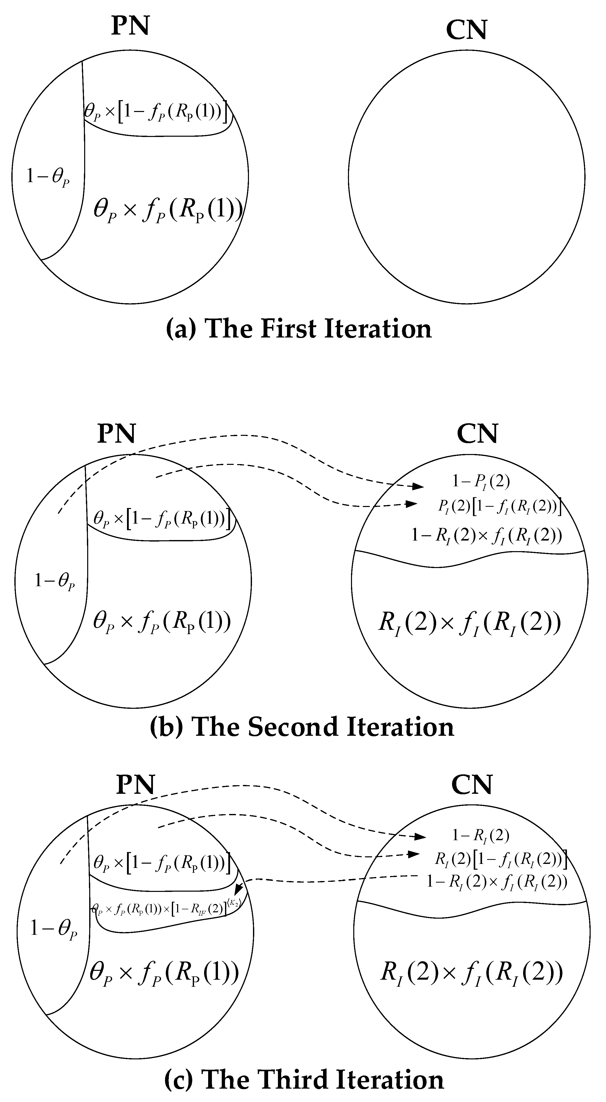
Appendix C. Analysis of Cross-Domain Cascading Failures

The first iteration N=1 of the CCF is shown in Equation (A29).
{ R P ( 1 ) = 1 θ P R P F ( 1 ) = R P ( 1 ) × f P ( R P ( 1 ) ) .
The number of nodes removed in the PN will further lead to failures of the corresponding nodes in the CN according to the power supply dependence relationship, and its number is shown in Equation (A30).
i = 1 N O N P × ( 1 R P F ( 1 ) ) O 2 i N O N P × ( 1 R P F ( 1 ) ) × O 2 .
The expected proportion of the failure of a power supply edge between the PN and CN is shown in Equation (A31).
N O N P × [ 1 R P F ( 1 ) ] × O 2 N O N P × O 2 = [ 1 R P F ( 1 ) ] .
Thus, the expected proportion of the node failure in the CN is shown in Equation (A32).
[ 1 R P F ( 1 ) ] O 1 .
Then the second iteration N=2 of the CCF is shown in Equation (A33).
{ R I ( 2 ) = 1 [ 1 R P F ( 1 ) ] O 1 R I F ( 2 ) = R I ( 2 ) × f I ( R I ( 2 ) ) .
When the number of nodes in the CN and the number of nodes in the PN are both large, the above equations hold.
The nodes in the CN with the expected proportion of 1 − RIF(2) fail. Among these failed nodes in the CN, the number of nodes belonging to the control nodes set VI3 is shown in Equation (A34).
N O N I × [ 1 R I F ( 2 ) ] × P r o b I ( V I 3 ) ,
where ProbI(VI3) = |VI3|/NONI.
The number of failure control edges which are owned by these failure nodes in the CN is shown in Equation (A35).
N O N I × [ 1 R I F ( 2 ) ] × P r o b I ( V I 3 ) × K 1 .
The total number of control edges is shown in Equation (A36).
N O N I × P r o b I ( V I 3 ) × K 1 .
Thus, the expected proportion of failure control edges is shown in Equation (A37).
N O N I × [ 1 R I F ( 2 ) ] × P r o b I ( V I 3 ) × K 1 N O N I × P r o b I ( V I 3 ) × K 1 = [ 1 R I F ( 2 ) ] .
Then the expected failure proportion of a node in the PN due to failure control edges is shown in Equation (A38).
[ 1 R I F ( 2 ) ] K 2 .
Then the corresponding expected proportion of a normal operational node in the PN due to failure control edges is shown in Equation (A39).
1 [ 1 R I F ( 2 ) ] K 2 .
According to the assumption in literature [26], then the third iteration N=3 of the CCF is shown in Equation (A40).
{ R P ( 3 ) = ( 1 θ P ) × [ 1 ( 1 R I F ( 2 ) ) K 2 ] R P F ( 3 ) = R P ( 3 ) × f P ( R P ( 3 ) ) .

Appendix D. A Special Case of Evaluation <O1> and <O2>

For a node nPi belonging to the substation node set VP2 in the PN of the ADN, it is assumed that the number of nodes in the CN that the node nPi can supply power is proportional to the degree of this node nPi [23]. The specific relationship is shown in Equation (A41).
O 2 ( n P i ) = μ P d P ,
where μP is constant. The expected number of nodes in the CN is supplied by a node nPi in the PN is shown in Equation (A42).
O 2 ( n P i ) = d P = 0 P r o b P ( d P ) × μ P d P = μ P d P ,
where ProbP(dP) represents the probability of a node nPi with a degree dP belonging to the substation node set VP2. <dP> represents the average node degree in the substation node set VP2.
The probability that only one node nIj in the CN will receive power from a node nPi with a degree dP belonging to the substation node set VP2 in the PN is shown in Equation (A43).
Pr o b P ( O 2 ( n P i ) = 1 ) = O 2 ( n P i ) × P r o b P ( d P ) | V P 2 | × < O 2 ( n P i ) > .
Then, the probability that o nodes in the CN will receive power from a node nPi with a degree dP belonging to the substation node set VP2 in the PN is shown in Equation (A44).
P r o b P ( O 2 ( n P i ) = o ) = ( d P o ) ( N o N I o ) × P r o b P ( O 2 ( n P i ) = 1 ) o × [ 1 P r o b P ( O 2 ( n P i ) = 1 ) ] N O N I o
where o is less than or equal to dP.
Furthermore, the probability that an arbitrary node nPi belonging to the substation node set VP2 in the PN supplies power to o nodes in the CN can be obtained as shown in Equation (A45).
P r o b P ( O 2 = o ) = d P = 0 P r o b P ( O 2 ( n P i ) = o ) × P r o b P ( d P ) .
Finally, the expected number of nodes in the CN is power supplied by any one node in the substation node set VP2 in the PN is shown in Equation (A46).
O 2 = o = 1 N O N I o × P r o b P ( O 2 = o ) .
The expected number of nodes belonging to the substation node set VP2 in the PN which supplies power to any one node in the CN is derived in a similar way. The probability that any one communication node is powered by o nodes belonging to the substation node set VP2 in the PN is shown in Equation (A47).
P r o b I ( O 1 = o ) = ( 1 | V P 2 | × O 2 ) o .
Thus, the expected number of nodes belonging to the substation node set VP2 in the PN which supplies power to any one node in the CN is shown in Equation (A48).
O 1 = o = 1 | V P 2 | o × P r o b ( O 1 = o ) .
The process of obtaining other quantities such as <K1>, <K2>, <L1>, and <L2> is similar.

Appendix E. A Proof of Proposition 1

Proof: According to Equation (A6), if the tolerance parameter αP of the node in the power network is bigger, then the probability ProbP(EvtP3/DP1 = dPO2) is smaller. Correspondingly, according to Equations (A9) and (A14), it can be seen that the probability ProbP(Evt′P2/EvtP1) is smaller as well. Then according to Equation (A13), fP(1 − ΘP) becomes bigger as the tolerance αP of the node in the power network is bigger. As the tolerance αP→∞, ProbP(EvtP3/DP2 = d′P)→0, ProbP(EvtP3/DP1 = dPO2)→0, and then the Equation (A49) can be obtained.
lim α P f P ( 1 θ P ) = d P = max { 0 , O 2 } P r o b P ( d P ) × ( 1 P r o b P ( E v t P 2 E v t P 1 ) d P O 2 ) .
According to Equation (A49) and Equation (6), if RP(2N + 1) ≠ 0, RPF(2N + 1) ≠ 0, RI(2N) ≠ 0, and RIF(2N) ≠ 0, then RP(2N + 1), RPF(2N + 1), RI(2N), and RIF(2N) will be bigger. Therefore the expected proportions RPF(2N + 1) of the remaining normal operational nodes reach their upper limits, which are the results of a pure interdependence model without considering the load redistribution. The similar proof process applies to the expected proportions RIF(2N) of the remaining normal operational nodes in the communication network.

References

  1. Bollen, M.H.J.; Sannino, A. Voltage control with inverter-based distributed generation. IEEE Trans. Power Deliv. 2005, 20, 519–520. [Google Scholar] [CrossRef]
  2. Fuangfoo, P.; Lee, W.J.; Kuo, M.T. Impact study on intentional islanding of distributed generation connected to radial subtransmission system in Thailand’s electric power system. In Proceedings of the Conference Record of the 2006 IEEE Industry Applications Conference Forty-First IAS Annual Meeting, Tampa, FL, USA, 8–12 October 2006; pp. 1140–1147. [Google Scholar] [CrossRef]
  3. Ochoa, L.F.; Dent, C.J.; Harrison, G.P. Distribution network capacity assessment: Variable DG and active networks. IEEE Trans. Power Syst. 2010, 25, 87–95. [Google Scholar] [CrossRef]
  4. Sridhar, S.; Hahn, A.; Govindarasu, M. Cyber-Physical System Security for the Electric Power Grid. Proc. IEEE 2012, 100, 210–224. [Google Scholar] [CrossRef]
  5. Vespignani, A. Complex networks: The fragility of interdependency. Nature 2010, 464, 984–985. [Google Scholar] [CrossRef] [PubMed]
  6. Huang, Z.; Wang, C.; Stojmenovic, M.; Nayak, A. Characterization of cascading failures in interdependent cyber-physical systems. IEEE Trans. Comput. 2015, 64, 2158–2168. [Google Scholar] [CrossRef]
  7. Rahnamay-Naeini, M.; Hayat, M.M. Cascading failures in interdependent infrastructures: An interdependent Markov-chain approach. IEEE Trans. Smart Grid 2016, 7, 1997–2006. [Google Scholar] [CrossRef]
  8. Chen, Y.; Li, Y.; Li, W.; Wu, X.; Cai, Y.; Cao, Y.; Rehtanz, C. Cascading Failure Analysis of Cyber-physical Power System With Multiple Interdependency and Control Threshold. IEEE Access 2018, 6, 39353–39362. [Google Scholar] [CrossRef]
  9. Sun, Y.; Tang, X. Cascading failure analysis of power flow on wind power based on complex network theory. J. Mod. Power Syst. Clean Energy 2014, 2, 411–421. [Google Scholar] [CrossRef]
  10. Yan, J.; Zhu, Y.; He, H.; Sun, Y. Multi-contingency cascading analysis of smart grid based on self-organizing map. IEEE Trans. Inf. Forensics Secur. 2013, 8, 646–656. [Google Scholar] [CrossRef]
  11. Scala, A.; Pahwa, S.; Scoglio, C. Cascade Failures from Distributed Generation in Power Grids. Int. J. Crit. Infrastruct. 2015, 2, 27–35. [Google Scholar] [CrossRef]
  12. Zhang, X.; Chi, K.T. Assessment of robustness of power systems from a network perspective. IEEE Trans. Emerg. Sel. Top. Circuits Syst. 2015, 5, 456–464. [Google Scholar] [CrossRef]
  13. Athari, M.H.; Wang, Z. Impacts of Wind Power Uncertainty on Grid Vulnerability to Cascading Overload Failures. IEEE Trans. Sustain. Energy 2017, 9, 128–137. [Google Scholar] [CrossRef]
  14. Tu, H.; Xia, Y.; Iu, H.H.C.; Chen, X. Optimal robustness in power grids from a network science perspective. IEEE Trans. Circuits Syst. 2019, 66, 126–130. [Google Scholar] [CrossRef]
  15. Buldyrev, S.V.; Parshani, R.; Paul, G.; Stanley, H.E.; Havlin, S. Catastrophic cascade of failures in interdependent networks. Nature 2010, 464, 1025–1028. [Google Scholar] [CrossRef] [PubMed]
  16. Shao, J.; Buldyrev, S.V.; Havlin, S.; Stanley, H.E. Cascade of failures in coupled network systems with multiple support-dependence relations. Phys. Rev. E 2011, 83, 036116. [Google Scholar] [CrossRef]
  17. Huang, Z.; Wang, C.; Stojmenovic, M.; Nayak, A. Balancing system survivability and cost of smart grid via modeling cascading failures. IEEE Trans. Emerg. Top. Comput. 2013, 1, 45–56. [Google Scholar] [CrossRef]
  18. Pinnaka, S.; Yarlagadda, R.; Çetinkaya, E.K. Modelling robustness of critical infrastructure networks. In Proceedings of the 2015 11th International Conference on the Design of Reliable CNs (DRCN), Kansas City, MO, USA, 24–27 March 2015; pp. 95–98. [Google Scholar] [CrossRef]
  19. Chai, W.K.; Kyritsis, V.; Katsaros, K.V.; Pavlou, G. Resilience of interdependent communication and power distribution networks against cascading failures. In Proceedings of the 2016 IFIP Networking Conference (IFIP Networking) and Workshops, Vienna, Austria, 17–19 May 2016; pp. 37–45. [Google Scholar] [CrossRef]
  20. La, R.J. Cascading failures in interdependent systems: Impact of degree variability and dependence. IEEE Trans. Netw. Sci. Eng. 2018, 5, 127–140. [Google Scholar] [CrossRef]
  21. Parshani, R.; Buldyrev, S.V.; Havlin, S. Critical effect of dependency groups on the function of networks. Proc. Natl. Acad. Sci. USA 2011, 108, 1007–1010. [Google Scholar] [CrossRef]
  22. Rahnamay-Naeini, M.; Hayat, M.M. On the role of power-grid and communication-system interdependencies on cascading failures. In Proceedings of the 2013 IEEE Global Conference on Signal and Information Processing, Austin, TX, USA, 3–5 December 2013; pp. 527–530. [Google Scholar] [CrossRef]
  23. Huang, Z.; Wang, C.; Zhu, T. Cascading failures in smart grid: Joint effect of load propagation and interdependence. IEEE Access 2015, 3, 2520–2530. [Google Scholar] [CrossRef]
  24. Cai, Y.; Cao, Y.; Li, Y.; Huang, T.; Huang, T. Cascading failure analysis considering interaction between power grids and communication networks. IEEE Trans. Smart Grid 2016, 7, 530–538. [Google Scholar] [CrossRef]
  25. Chen, Z.; Wu, J.; Xia, Y.; Zhang, X. Robustness of interdependent power grids and communication networks: A complex network perspective. IEEE Trans. Circuits Syst. II Exp. Briefs 2018, 65, 115–119. [Google Scholar] [CrossRef]
  26. Huang, Z.; Wang, C.; Nayak, A.; Stojmenovic, I. Small cluster in cyber-physical systems: Network topology, interdependence and cascading failures. IEEE Trans. Parallel Distrib. Syst. 2015, 26, 2340–2351. [Google Scholar] [CrossRef]
  27. Han, Y.; Guo, C.; Ma, S.; Song, D. Modeling cascading failures and mitigation strategies in PMU based cyber-physical power systems. J. Mod. Power Syst. Clean Energy 2018, 6, 944–957. [Google Scholar] [CrossRef]
  28. Dobson, I.; Carreras, B.A.; Lynch, V.E.; Newman, D.E. Complex systems analysis of series of blackouts: Cascading failure, critical points, and self-organization. Chaos 2007, 17, 026103. [Google Scholar] [CrossRef]
Figure 1. A brief architecture of an active distribution network (ADN).
Applsci 09 05021 g001
Figure 2. Simple running example of a cross-domain cascading failure (CCF) in an ADN.
Applsci 09 05021 g002
Figure 3. Venn diagram for computing RPF(N)/RIF(N) in the first three iterations.
Applsci 09 05021 g003
Figure 4. The UCTE (Union for the Co-ordination of Transmission of Electricity) summer case data 2002 curve using MATCASC (cascading line outages analyse tool for power grids).
Applsci 09 05021 g004
Figure 5. The final expected proportion of normal operational nodes in the power network (PN) after the CCF stops (RPF(∞)) of different distributed generators proportions in the PN with Erdos–Renyi (ER) topological structure.
Applsci 09 05021 g005
Figure 6. RPF(∞) of different distributed generators proportions in the PN with Barabasi–Albert (BA)topological structure.
Applsci 09 05021 g006
Figure 7. The final expected proportion of normal operational nodes in the PN/communication network (CN) after the CCF stops (RPF(∞)/RIF(∞)) of different ΘP in the PN and CN with the ER topological structure.
Applsci 09 05021 g007
Figure 8. RPF(∞)/RIF(∞) of different independence between the PN and CN.
Applsci 09 05021 g008
Figure 9. Comparison of node degree distribution in the CN and PN.
Applsci 09 05021 g009
Figure 10. RPF(∞)/RIF(∞) of different network topology under different proportion of distributed generators and the unintentional-random-initial-failure-rate ΘP= 0.002.
Applsci 09 05021 g010
Figure 11. RPF(∞)/RIF(∞) of different network topology under different ΘP and proportion of distributed generators = 0.8.
Applsci 09 05021 g011
Figure 12. RPF(∞)/RIF(∞) of different tolerance parameters in the PN and CN.
Applsci 09 05021 g012
Table 1. Notation used in this paper.
SymbolDescription
GAActive distribution networks (ADNs).
GPThe power networks of the ADN.
GIThe communication networks of the ADN.
VPThe nodes set of the PN.
VIThe nodes set of the CN.
NoNPThe number of the nodes in the PN.
NoNIThe number of the nodes in the CN.
Vf-initialThe unintentional random initial failure nodes set of the PN.
The steady-state of the ADN after the CCF.
GP1(), GP2(),…
SP(Vf-initial, )
The connected clusters in the PN of the ADN after the CCF stops.
GPg1(), GPg2(),…
SPg(Vf-initial, )
The connected clusters containing generators in the PN of the ADN after the CCF stops.
GI1(), GI2(),…
SI(Vf-initial, )
The connected clusters in the CN of the ADN after the CCF stops.
GIg1(), GIg2(),…
SIg(Vf-initial, )
The connected clusters in the CN are interdependent with the connected clusters containing generators in the PN of the ADN after the CCF stops.
NumThe number of experiments.
NThe number of iterative steps in the propagation of the CCF.
RP(N)/RI(N)The expected proportion of remaining nodes in the PN/CN at step N after the CCF occurs.
fP(RP(N))The expectation of the quotient between the number of the remaining nodes in the clusters that containing generators and the number of the remaining nodes of the whole PN at step N after the CCF occurs.
fI(RI(N))The expectation of the quotient between the number of the remaining nodes belonging to the connected clusters in the CN interdependent with the connected clusters containing generators in the PN and the number of the remaining nodes of the whole CN at step N after the CCF occurs.
RPF(N)/RIF(N)The expected proportion of normal operational nodes in the PN/CN at step N after the CCF occurs.
RPF()/RIF()The final expected proportion of normal operational nodes in the PN/CN after the CCF stops.
ΘPThe probability that a single node in the PN fails randomly.
EdgP(n)/EdgI(n)The edge set (excluding the edges connecting the PN and the CN) of a node n in the PN/CN.
<K2>The average control fan in of a node in the PN.
<O1>The average power fan in of a node in the CN.
BCtrlThe set of the paths involved in an effective control EconI.
TPL(e)/TIL(e)Load threshold of an edge e in the PN/CN.
Run(n)/¬Run(n)A node or an edge n runs normally/ abnormally.
αP/αIA tolerance parameter of a node n in the PN/CN which represents the ratio of the maximum capacity to nominal capacity of the node n.
Table 2. Normal operation conditions.
DomainTypeNormal Operation Conditions
PNNode
nP
(1)
It is connected to at least one power generation node nPP in the PN, i.e.,
( n P P ( V P 1 V P 5 ) ) . p a t h ( n P , n P P )
(2)
It has at least one edge between the node nP in the PN and a node nII in the CN, and the node nII is part of at least one path in the set Btr. i.e.,
n I I . ( ( n P , n I I ) E P I ) ( p a t h ( n I I , n I 4 ) B t r )
(3)
The load flowing through this node nP does not exceed its threshold TPP(nP) at step N. i.e.,
( l o a d ( n P , N ) T P P ( n P ) ) ( n P V P )
Edge
eP
(1)
The load flowing through the edge eP does not exceed its threshold TPL(eP) at step N. i.e.,
( l o a d ( e P , N ) T P L ( e P ) ) ( e P E P )
(2)
The nodes on both sides of the edge eP are in normal operation. i.e.,
( e P = ( n P x V P , n P y V P ) ) ( r u n ( n P x ) r u n ( n P y ) )
CNNode
nI
(1)
There is at least one normal operating node np in the PN that provides power to this node nI. i.e.,
n P . ( ( e = ( n P V P , n I V I ) ) r u n ( n P ) )
(2)
The data traffic of this node nI in the CN does not exceed its threshold at step N. i.e.,
( l o a d ( n I , N ) , n I V I ) T I P ( n I )
(3)
The node nI is part of at least one path in the set Btr. i.e.,
n I 4 . p a t h ( n I , n I 4 ) B t r
Edge
eP
(1)
The load (data packets) flowing through the edge eP does not exceed its threshold TIL(eP) at step N. i.e.,
( l o a d ( e P , N ) T I L ( e P ) ) ( e P E I )
(2)
The nodes on both sides of edge eP are in normal operation. i.e.,
( e P = ( n I x V I , n I y V I ) ) ( r u n ( n I x ) r u n ( n I y ) )
The interdependence between the PN and the CNEdge
e
(1)
The nodes on both sides of the edge e ∈ (EPIEIP) are in normal operation. i.e.,
( ( e = ( n P P x V P , n I I x V I ) ) ( e = ( n I I x V I , n P P x V P ) ) ) ( r u n ( n P P x ) r u n ( n I I x ) )

