Featured Application
The method can be used in such areas as optical wave reconstruction, three dimensional microscopic imaging, and interference measurement.
Abstract
A convenient and powerful method is proposed and presented to find the unknown phase shifts in three-step generalized phase-shifting interferometry. A slight-tilt reference of 0.1 degrees is employed. As a result, the developed theory shows that the unknown phase shifts can be simply extracted by subtraction operations. Also, from the theory developed, the tilt angle of the tilt reference can also be calculated, which is important as it allows us to extract the object wave precisely. Numerical simulations and optical experiments were performed to demonstrate the validity and efficiency of the proposed method. The proposed slight-tilt reference allows the full and efficient use of the space-bandwidth product of the limited resolution of digital recording devices as compared to the situation in standard off-axis holography where typically several degrees for off-axis angle is employed.
1. Introduction
Phase-shifting interferometry (PSI) has been developing for decades and applied to many fields [1,2,3,4,5,6]. In the development of PSI techniques, there is a transition from the traditional fixed phase shifts to random unknown phase shifts [7,8]. In general, the phase shift of the reference beam introduced into the PSI is typically affected by environmental interference and phase shifter errors [9]. To further simplify the measurement procedures and avoid the negative effects of the environmental disturbances and phase shifter errors, Cai et al. have introduced generalized phase-shifting interferometry (GPSI), where the phase shifts are generally arbitrary, unequal and unknown values, but can be extracted from several interferograms [10,11]. Yoshikawa et al. later have developed GPSI by using statistical distribution of the diffracted wave and normalized holograms [12,13,14]. To achieve further convenience, non-iterative methods [11,15,16,17,18] begin to replace the iterative methods, which always need a long computation time, and sometimes it is difficult to make the extracted values convergent. However, complicated equations and tedious operations in these phase shift extraction processes give rise to some inconvenience in the application of GPSI.
In recent years, interference with a tilt reference [18,19] has been proposed in digital holography for monitoring purposes. In order to improve the convenience and stability of the phase-shift extracting algorithm further in three-step PSI, we propose a simpler and more reliable method to extract the unknown phase shifts with a slightly tilted reference beam during the recording process.
Three-step generalized phase-shifting interferometry (TGPSI) uses three interferograms to extract phase shifts and retrieve the original object wave. In GPSI research, TGPSI can retrieve the object wave stably by only three holograms without any additional measurements. In this paper, we propose the use of a slightly tilted reference so that the extraction of the phase shift can become simpler and more stable without iteration. We derive the theory behind the proposed method and carry out numerical simulations as well as optical experiments to verify our idea.
2. Basic Principle
In the TGPSI method, the complex amplitudes of object wave and reference wave on the recording plane can be written as
where for brevity, we have assumed Ar to be constant. Obviously, in Equation (2) the phase of the tilt reference plane wave φr(x, y) is not a constant but a linear distribution on recording plane given by
where is the wavelength of the laser and and are the off-axis angles along the x and y directions. From Equations (1) and (2), the intensities for the three interferograms are described by
where and are unknown phase shifts that need to be determined. Subtracting Equations (5) and (6) from Equation (4) respectively, we have
From Equations (7) and (8), we derive the following expressions:
which are the imaginary and the real parts of the following complex amplitude:
Substituting Equations (9) and (10) into (11), we have
Note that from Equation (11), we can see that this complex field is related to the original object wave (see Equation (1)) as follows:
In order to extract , we, therefore, need to know and . Let us first concentrate on finding . According to Equation (12), can be found with known intensities I1, I2, I3 along with unknown, to be determined, phase shifts and .
It is known that the precise extraction of phase shifts and is critical to the reconstruction of the object wave. In TGPSI, many time-consuming iterative algorithms are used to search for the actual values of the phase shift. We propose a powerful and reliable method to extract phase-shift values based on the theory developed so far. To this end, we first analyze the spectrum of the interferograms. Equations (4)–(6) can be rewritten as
in order to obtain phase shifts and , Fourier transform (FT) operations on Equations (14)–(16) are needed, and they are
where symbol ‘*’ presents the conjugate operation. F1(u, v), F2(u, v) and F3(u, v) are the Fourier transforms of I1, I2 and I3, respectively. The first term FA(u, v) in the right side of Equations (17)–(19) is the spectrum of the object intensity, distributing in the central part of the spectrum plane. Because the reference intensities Ir is a constant, the second term of the three equations give a δ-function, showing a bright point at the origin (0, 0) on the spectrum plane. The last two terms in the right side of Equations (17)–(19) are the shifted spectra of the object wave and its conjugate, where FO(u + up, v + vp) is the Fourier transform of Aoexp(−iφo)exp(iφr) and FO*(−u + up,−v + vp) is the Fourier transform of Aoexp(iφo)exp(−iφr). They are confined in two relatively small areas, but the centers are shifted to points (−up, −vp) and (up, vp) on the spectrum plane due to the tilt reference employed. In some cases of complicated object wave, points (−up, −vp) and (up, vp) may be difficult to locate as they are hidden within the spectra of FO(u + up, v + vp) or FO*(−u + up, −v + vp) due to the slight-tilt reference angle (fraction of a degree). However, we can perform interference of two plane waves as the spectrum of such interference contains δ-functions centered at (0,0), (−up, −vp), and (up, vp), which can be found easily. After (−up, −vp), and (up, vp) are determined, the spectrum at these points can be used to extract unknown phase shifts Δφr1 and Δφr2, to be explained below. Indeed, if we isolate the spectra at points (−up, −vp) and (up, vp) in the third term of Equations (17) and (18), we have and , respectively can be extracted by subtracting the argument of the above two terms and by evaluating at and to give:
Alternatively, we can also use their conjugate terms, i.e., and . However, in this case, we need to evaluate the terms at and to give .
Similarly, we extract from the third terms of Equations (18) and (19). Again, we use and , and we find
where arg [ . ] in the above equations denotes taking the argument of a complex value in the square bracket. Equations (20) and (21) use only a simple subtraction operation to extract unknown phase shifts and without any iteration. This is the first contribution of using the proposed small-tilt reference.
Our next goal is to find object wave . Now with and already extracted, we can calculate from Equation (12). and are related by Equation (13) through as follows:
We can calculate off-axis angles and by the following relationships [1]
where M and N are the total pixel numbers along the horizontal and vertical directions of the hologram. dx and dy are the corresponding pixel size in the two directions. Note that we have been using normalized spatial frequencies, u and v. Hence up and vp are divided by the total length of the Charge-coupled Device (CCD) linear dimension, Mdx and Mdy. Since up and vp have already been located, we can determine the off-axis angles. Once the angles are found, object wave is completely determined from Equation (22), and finally the complex amplitude of the original object can be calculated by performing backward Fresnel diffraction [1].
The whole process of the proposed new algorithm for finding the unknown phase shifts and object wave reconstruction can be summarized in the following steps:
Step 1: Set and determine the reference tilt angle before the test object is put in the optical path. Experimentally, we fix the tilt angle when dozens of fringes appear on the CCD from the interference of two plane waves. We label I0 as the intensity pattern of the interference between the two plane waves. We then put in the object and record I1, I2 and I3.
Step 2: Perform FT operations on the fringe pattern from the plane wave interference in Step 1 and search the brightest points on the spectral plane (not the point at the origin of the spectral plane) and locate the coordinates of the found points as (−up, −vp) or (up,vp). Perform FT operations on I1, I2 and I3 and store the complex values of these two points. In most practical situations, (−up, −vp) or (up, vp) can also be found from the spectrum of either one of I1, I2 and I3 without the need of two-plane wave interference.
Step 3: Calculate phase shift and by Equations (20) and (21) using the values stored in step 2.
Step 4: Reconstruct by Equation (12).
Step 5: Find the tilt angle by Equation (23) from the located coordinates of (−up, −vp) or (up, vp).
Step 6: Find by using Equation (22).
Step 7: Recover the original object image by backward Fresnel diffraction of .
3. Computer Simulation and Optical Experiments
3.1. Computer Simulation
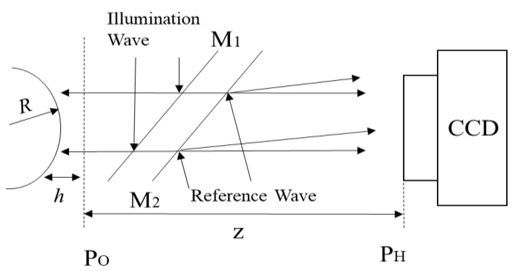
We have carried out a series of computer simulations to verify the effectiveness of the proposed method before any optical experiments. In these simulations, many elliptical surfaces with different parameters have been used as reflecting target objects. A plane wave of 532 nm illuminates these surfaces and is then reflected back onto the CCD in the recording setup illustrated in Figure 1.

Figure 1.
Simulation setup in phase-shifting digital holography with the tilted reference wave.
In the simulation setup in Figure 1 [20], there were 512 × 512 pixels with 15 μm × 15 μm size on the CCD and the recording distance was set as z = 216.5 mm (all the parameters satisfy the sampling theory to avoid aliasing [1]). With the paraxial approximation of an elliptical wave, we set the phase distribution on the original object plane Po, which is tangential to the surface at the vertex, as 4πh(x,y)/λ, with h the surface depth determined by radius of curvature R. We used
Accounting for the possible amplitude variation of an object wave, a Gaussian amplitude intensity distribution of the object wave in plane Po was introduced, decreasing gradually from the center of maximum 1 to the edge of minimum 0.7. Two-dimensional Fresnel diffraction makes the complex amplitude in plane Po give the object wave , in the recording plane PH. Three different interferograms by two reference phase shifts are computer-generated. In this simulation we set two phase-shift values of 1 and 0.6 rad respectively, and we give only a few results with R = 2000 mm as example. The reference wave is a plane wave with a slight tilt angle along both the x-axis and the y-axis.
As for optical experimental procedures, in order to accurately determine the small tilt angle of the reference light, we introduce a plane wave as the object wave to obtain I0. We control the tilt angle of the reference until there are dozens of fringes appearing on the CCD. We then obtain the corresponding spectrum to find (−up, −vp) and (up, vp).
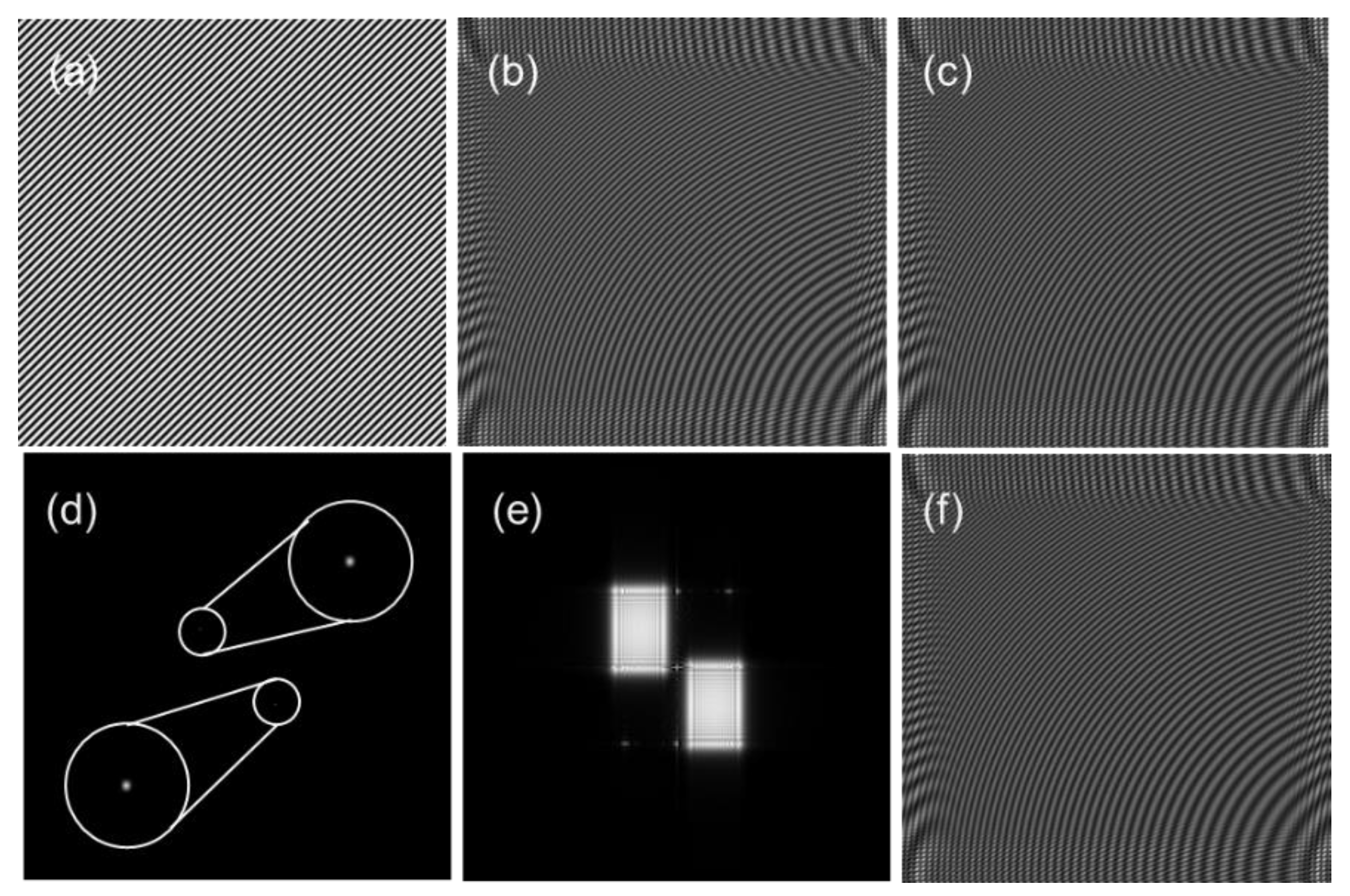
Fast Fourier Transform (FFT) operations are carried out on the interferograms on the computer. Figure 2a shows the pattern of and its corresponding spectrum is shown in Figure 2d. The two delta functions are located at (−up, −vp) and (up,vp), which have been zoomed in for visual inspection. Figure 2b shows the pattern of and its corresponding spectrum is shown in Figure 2e. Note that the zero frequency has been suppressed for display purposes in Figure 2d,e. Figure 2c,f show the pattern of and , respectively.
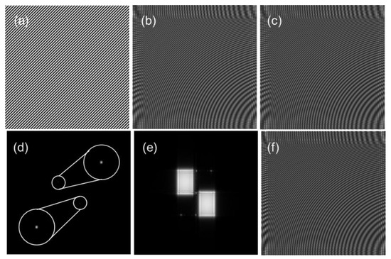
Figure 2.
Simulation results: (a) I0; (b) I1; (c) I2; (d) spatial spectrum of I0; (e) spatial spectrum of I1; (f) I3.
By searching the maximum value of the spectrum intensity from the FT of I0, coordinates (−up, −vp) and (up, vp) are found to be (−45, 45) and (45, −45). Substituting up = 45, vp = 45, λ = 0.532 μm, dx = 15 μm, dy = 15 μm and M = N = 512 into Equation (23), the reference wave angles in the x and y directions are found to be both approximately 0.18 degrees. After the spectrum coordinates (−up, −vp) and (up, vp) are found, the phase angle of the complex values of the spectra at pixel (−45, 45) or (45, −45) can be calculated and then the two phase shifts are extracted by subtraction operation using Equations (20) and (21).
The phase shifts, and , calculated by our proposed method are 1.0002 rad and 0.6003 rad, respectively. The two phase shifts with errors of 0.0002 and 0.0003 rad are accurate enough in the non-iterative GPSI method. These phase shift errors come from the digital resolution on the FT spectral plane.
Using the three interferograms and the two extracted phase shifts, wavefront is retrieved through Equation (12) and then corrected by Equation (22) with the tilt angles of about θx = 0.18 degrees and θy = 0.18 degrees. Back Fresnel diffraction was carried out to obtain the object on the object plane.
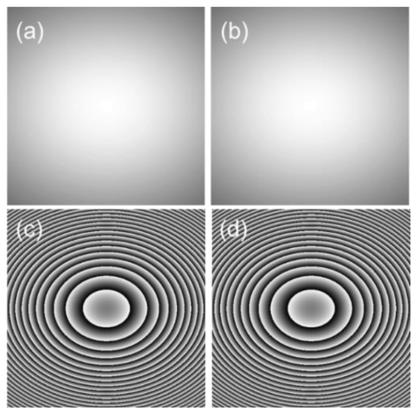
Figure 3a,b shows the amplitude distributions for the original object wave and the reconstructed object wave. In the simulation setup, the intensity distribution was designed as a Gaussian function to simulate an object wave amplitude. That is to say, the object wave recorded has not only phase distribution but also amplitude variation. Although the amplitude of the original object wave is not uniform, the proposed method can recover it ideally, because there is almost no difference between Figure 3a,b. The phase of the original object wave and its reconstructed phase are shown in Figure 3c,d, respectively. It is difficult for us to find any difference between the two figures.
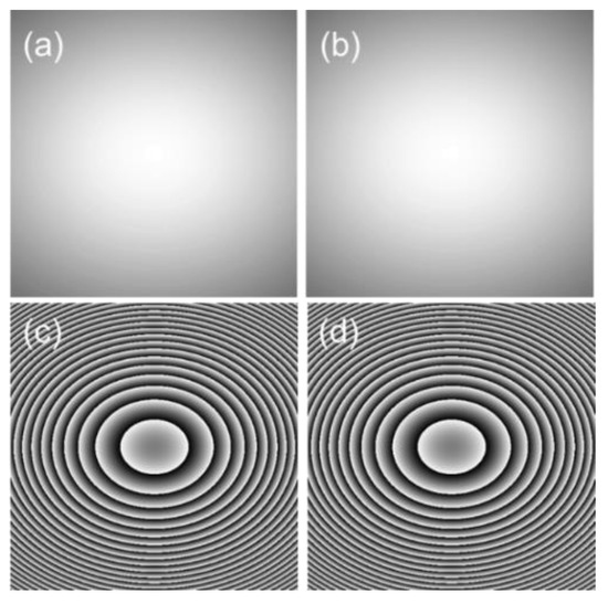
Figure 3.
Simulation results: (a) intensity of the original object wave; (b) intensity of reconstructed object wave; (c) original phase distribution; (d) reconstructed phase distribution.
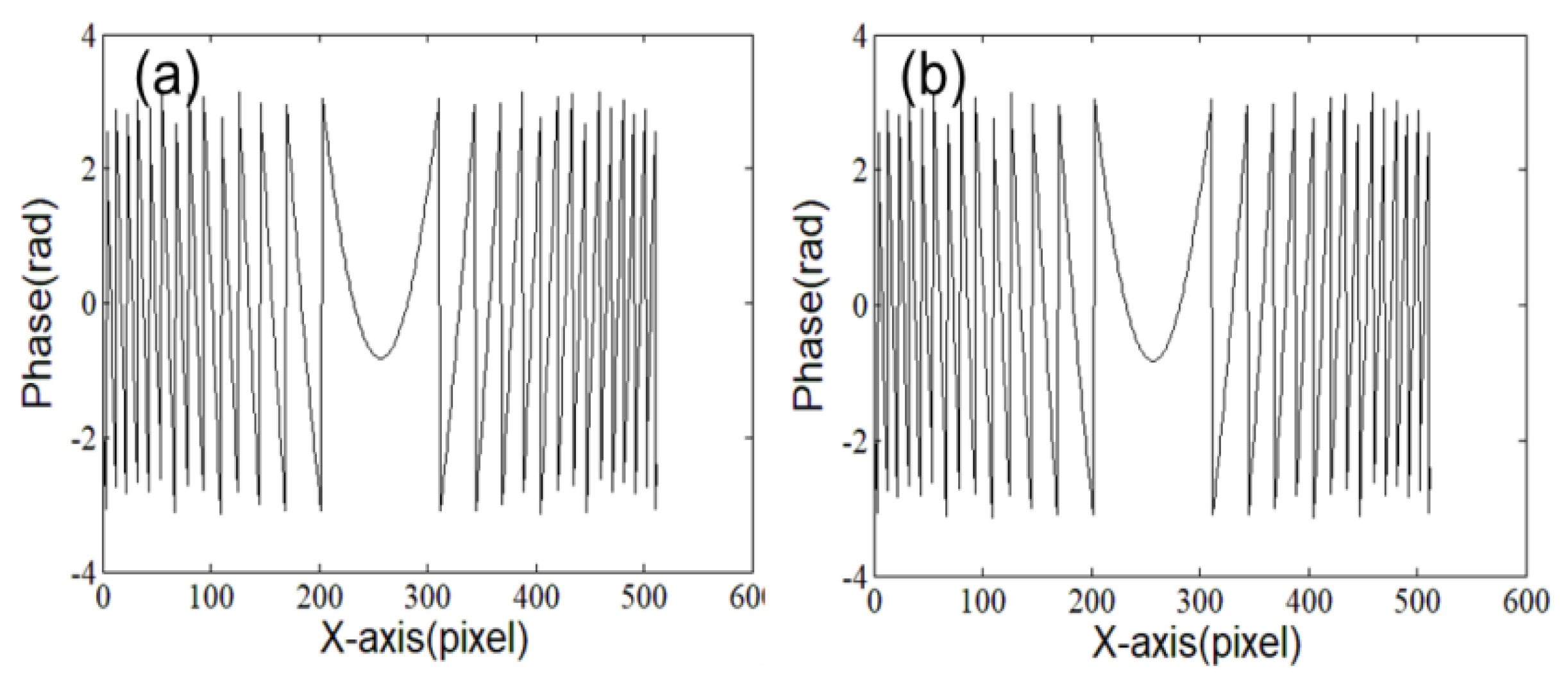
To inspect the phase distribution of the object wave quantitatively, the phase across the center of the zones are plotted in Figure 4. For comparison, the original phase and the reconstructed phase are shown in Figure 4a,b, respectively. Obviously Figure 4a,b are almost identical.
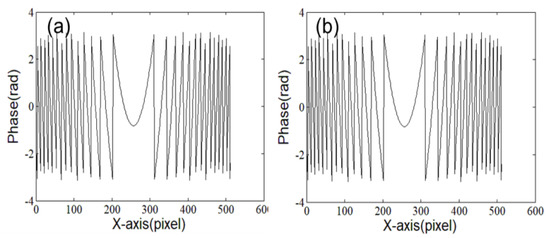
Figure 4.
Phase distribution across the center of the zones of the object wave, (a) original phase distribution and (b) reconstructed phase distribution.
3.2. Optical Experiment
Optical experiments have also been carried out with the optical setup shown in Figure 5 with a 532 nm laser, and the target object is a USAF resolution target. The CCD installed has a recording chip with a resolution of 1392 by 1040 pixels, and the pixel size is 6.45 × 6.45 μm.
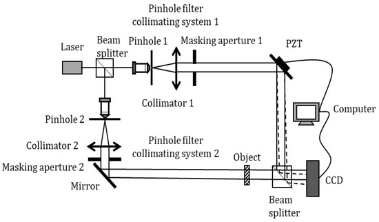
Figure 5.
Three-step generalized phase-shifting interferometry (TGPSI) recording setup with a slight-tilt reference, where the dotted lines illustrate the tilted reference actually used. A piezoelectric transducer (PZT) is used as a phase shifter.
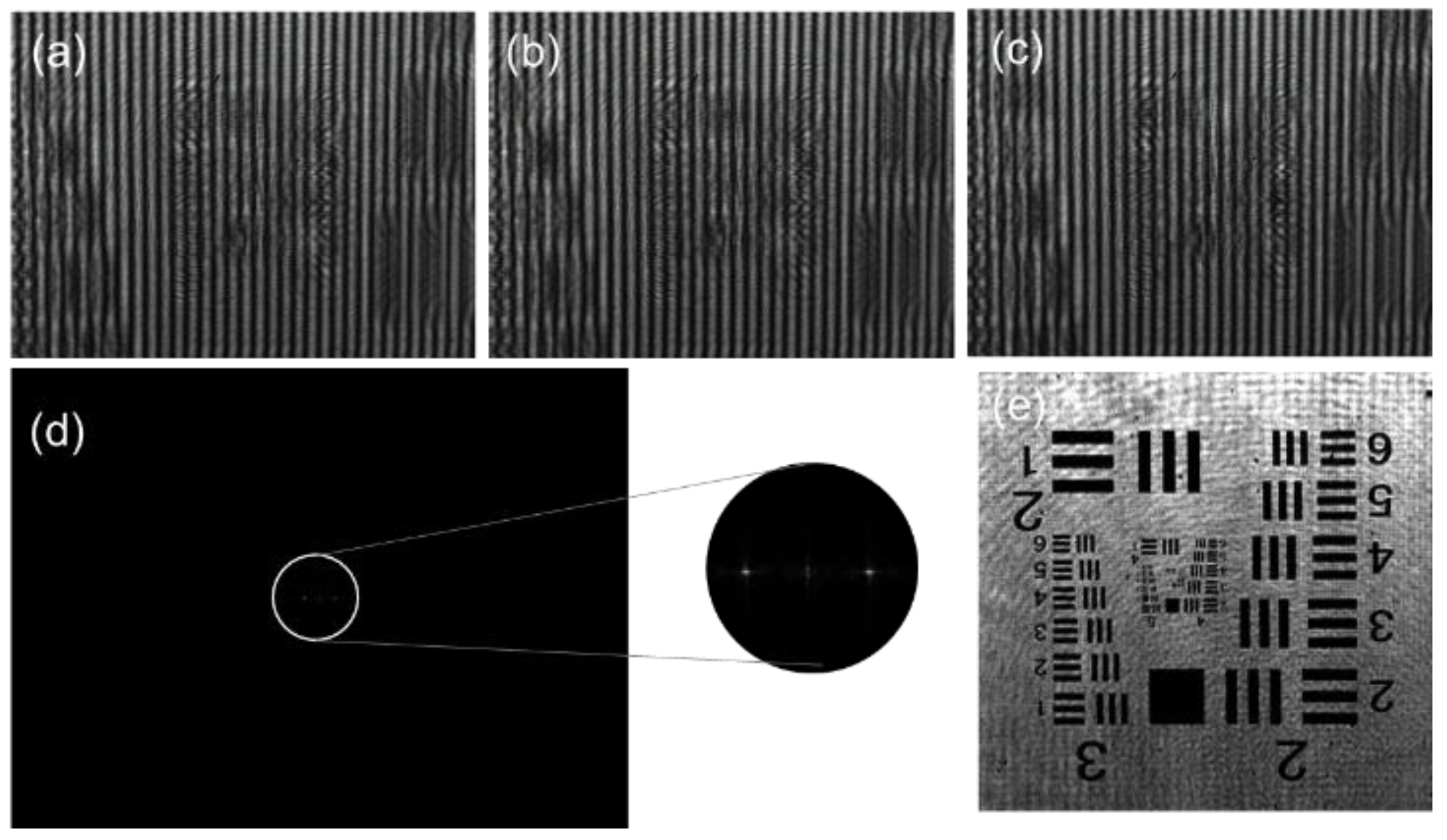
In our experiment, the phase shift is generated by a phase shifter. The results are illustrated in Figure 6. The three interferograms with unknown phase shifts are shown in Figure 6a–c. Figure 6d is the spectrum of Figure 6a, where the center part is enlarged and shown in the circle. We have used the spectrum of I1 instead of I0 to locate the coordinates (−up, −vp) and (up, vp) and they are found to be (−34, 0) and (34, 0). The reason is that there are two bright spots in the spectrum already. The enlarged portion of the spectrum clearly illustrates the two bright spots. Subsequently, the reference slight tilt angle can be calculated by Equation (23) and the result is about θx = 0.1 degree in the experiment. Phase shifts are calculated by using the brightest point at these locations on the three Fourier spectra of holograms I1, I2 and I3. The phase shifts calculated using the proposed method are 0.5211 and 1.8018 rad. Figure 6e is the intensity distribution of the reconstructed image, and the reconstructing distance is 10.9 cm. Both the accuracy of the phase shift extraction and the quality of the reconstructed image are excellent.
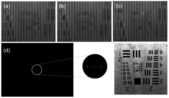
Figure 6.
Optical results (a) I1, (b) I2, (c) I3, (d) spectrum of I1 and (e) the reconstructed image.
4. Conclusions
We have proposed a method to extract unknown phase shifts in TGPSI with a slight-tilt reference. The major merit of the proposed method is that only two subtractions are used to calculate the unknown phase shifts. The technique is simple and yet powerful as no iteration is needed. It is convenient and accurate. The method needs only three interferograms to complete the phase shift extraction and wavefront reconstruction without iteration. Simulations and optical experiments have verified the feasibility and validity of the proposed method. It should be noted that this method works well when the zero-frequency component in the object spectrum is sufficiently large because the location of this spectrum is easy to find under such condition. For some extreme cases of complicated object waves, a slightly larger tilt angle is needed and the advantage of the efficient use of the space-bandwidth product is not obvious when this method is compared to the off-axis technique. This method is expected to be an attractive alternative for wide-ranging digital holography applications as it allows the full and efficient use of the space-bandwidth product of the limited resolution of digital recording devices because a slight tilt reference of 0.1 degrees is used.
Author Contributions
Conceptualization, X.X.; methodology, X.X., T.M. and Z.J.; software, X.X. and T.M.; validation, T.M. and L.X.; formal analysis, D.D. and F.Q.; investigation, X.X. and T.M.; resources, X.X.; data curation, T.M.; writing—original draft preparation, X.X. and T.M.; writing—review and editing, X.X. and T.-C.P.
Funding
This research was funded by the National Key Research and Development Program of China (2017YFC1404000), Natural Science Foundation of Shandong Province, China (ZR2019MD023) and Fundamental Research Funds for the Central Universities of China (15CX05033A).
Conflicts of Interest
The authors declare no conflict of interest.
References
- Poon, T.-C.; Liu, J.-P. Introduction to Modern Digital Holography with MATLAB; Cambridge University Press: Cambridge, UK, 2014. [Google Scholar]
- Bruning, J.H.; Herriott, D.R.; Gallagher, J.E.; Rosenfeld, D.P.; White, A.D.; Brangaccio, D.J. Digital wavefront measuring interferometer for testing optical surfaces and lenses. Appl. Opt. 1974, 13, 2693–2703. [Google Scholar] [CrossRef] [PubMed]
- Yamaguchi, I.; Zhang, T. Phase-shifting digital holography. Opt. Lett. 1997, 22, 1268–1270. [Google Scholar] [CrossRef] [PubMed]
- Xia, P.; Wang, Q.H.; Ri, S.; Tsuda, H. Calibrated phase-shifting digital holography based on a dual-camera system. Opt. Lett. 2017, 42, 4954–4957. [Google Scholar] [CrossRef] [PubMed]
- Zhang, J.Y.Z.; Ren, Y.J.; Zhu, Q.; Lin, Z.Q. Phase-shifting lensless Fourier-transform holography with a Chinese Taiji lens. Opt. Lett. 2018, 43, 4085–4087. [Google Scholar] [CrossRef] [PubMed]
- Wizinowich, P.L. Phase shifting interferometry in the presence of vibration: A new algorithm and system. Appl. Opt. 1990, 29, 3271–3279. [Google Scholar] [CrossRef] [PubMed]
- Xu, X.F.; Cai, L.Z.; Wang, Y.R.; Meng, X.F.; Zhang, H.; Dong, G.Y.; Shen, X.X. Blind phase shift extraction and wavefront retrieval by two-frame phase-shifting interferometry with an unknown phase shift. Opt. Commun. 2007, 273, 54–59. [Google Scholar] [CrossRef]
- Xu, J.C.; Xu, Q.; Chai, L.Q. Iterative algorithm for phase extraction from interferograms with random and spatially nonuniform phase shifts. Appl. Opt. 2008, 47, 480–485. [Google Scholar] [CrossRef] [PubMed]
- Guo, C.S.; Zhang, L.; Wang, H.T.; Liao, J.; Zhu, Y.Y. Phase-shifting error and its elimination in phase-shifting digital holography. Opt. Lett. 2002, 27, 1687–1689. [Google Scholar] [CrossRef] [PubMed]
- Cai, L.Z.; Liu, Q.; Yang, X.L. Generalized phase-shifting interferometry with arbitrary unknown phase steps for diffraction objects. Opt. Lett. 2004, 29, 183–185. [Google Scholar] [CrossRef] [PubMed]
- Xu, X.F.; Cai, L.Z.; Wang, Y.R.; Meng, X.F.; Sun, W.J.; Zhang, H.; Cheng, X.C.; Dong, G.Y.; Shen, X.X. Simple direct extraction of unknown phase shift and wavefront reconstruction in generalized phase-shifting interferometry: Algorithm and experiments. Opt. Lett. 2008, 33, 776–778. [Google Scholar] [CrossRef] [PubMed]
- Yoshikawa, N. Phase determination method in statistical generalized phase-shifting digital holography. Appl. Opt. 2013, 52, 1947–1953. [Google Scholar] [CrossRef] [PubMed]
- Yoshikawa, N.; Kajihara, K. Statistical generalized phase-shifting digital holography with a continuous fringe-scanning scheme. Opt. Lett. 2015, 40, 3149–3152. [Google Scholar] [CrossRef] [PubMed]
- Yoshikawa, N.; Namiki, S.; Uoya, A. Object wave retrieval using normalized holograms in three-step generalized phase-shifting digital holography. Appl. Opt. 2019, 58, A161–A168. [Google Scholar] [CrossRef] [PubMed]
- Zhang, S. A non-iterative method for phase-shift estimation and wave-front reconstruction in phase-shifting digital holography. Opt. Commun. 2006, 268, 231–234. [Google Scholar] [CrossRef]
- Xu, J.C.; Xu, Q.; Chai, L.Q.; Li, Y.; Wang, H. Direct phase extraction from interferograms with random phase shifts. Opt. Express 2010, 18, 20620–20627. [Google Scholar] [CrossRef] [PubMed]
- Guo, C.S.; Sha, B.; Xie, Y.Y.; Zhang, X.J. Zero difference algorithm for phase shift extraction in blind phase-shifting holography. Opt. Lett. 2014, 39, 813–816. [Google Scholar] [CrossRef] [PubMed]
- Xu, X.F.; Zhang, Z.W.; Wang, Z.C.; Wang, J.; Zhan, K.Y.; Jia, Y.L.; Jiao, Z.Y. Robust digital holography design with monitoring setup and reference tilt error elimination. Appl. Opt. 2018, 57, B205–B211. [Google Scholar] [CrossRef] [PubMed]
- Zeng, F.; Tan, Q.F.; Gu, H.R.; Jin, G.F. Phase extraction from interferograms with unknown tilt phase shifts based on a regularized optical flow method. Opt. Express 2013, 21, 17234–17248. [Google Scholar] [CrossRef] [PubMed]
- Cai, L.Z.; Liu, Q.; Yang, X.L. Phase-shift extraction and wave-front reconstruction in phase-shifting interferometry with arbitrary phase steps. Opt. Lett. 2003, 28, 1808–1810. [Google Scholar] [CrossRef] [PubMed]

© 2019 by the authors. Licensee MDPI, Basel, Switzerland. This article is an open access article distributed under the terms and conditions of the Creative Commons Attribution (CC BY) license (http://creativecommons.org/licenses/by/4.0/).