3.1. Monitoring of Data Center Physical Infrastructure
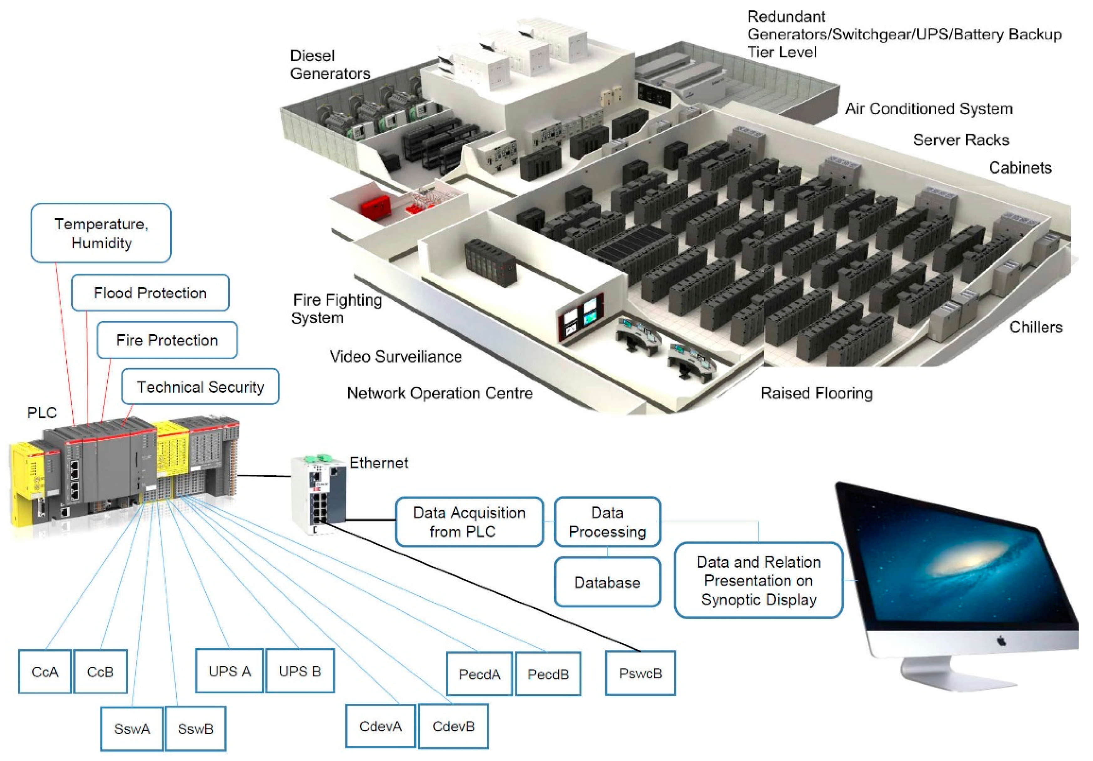
Figure 1 shows the typical data center technical infrastructure with diesel generators, power supplies, redundant power supplies, UPSs, a cooling system, an air-conditioned system, and technical safety. The status of individual devices in the data center technical infrastructure is obtained via various interfaces and sensors. Data are captured using a programmable logic controller (PLC) through various data capture interfaces (such as Ethernet, Wi-Fi, analog and digital interfaces) and stored in a database. In
Figure 1, CcA and CcB represent air conditioners. The purpose of the thermal management is to keep the temperatures in all room spaces below the upper limits required in the standard with the lowest energy consumption [
27]. The temperature for the A1 class should be in the range of 15–32 °C and the relative humidity should be between 20% and 80%, as shown in
Table 1 [
28]. To accurately measure the moisture and temperature in the data center technical infrastructure rooms, industrial humidity probes and sensors are used.
SswA and SswB are static transfer switches that have the task of transferring the power from UPS A to (UPS B) in the event of failure of the UPS A. CdevA and CdevB are cooling devices in which the chilled water temperature is allowed in range of 7.3–25.6 °C in accordance with the maximum allowed IT inlet air temperature, which was, in addition, used to calculate the chilled water temperature.
PecdA and PecdB represent cooling device power supplies, and PswcB is an interface for capturing the state of IT equipment power switches and circuit breakers.
Experimental equipment (Tier IV):
- -
6 EMERSON chillers (300 KW of cooling capacity each)—periodic autorotation of active versus
- -
standby (N + 2 redundancy), integrated free cooling;
- -
2 EuroDiesel rotary diesel UPSs (1340 KW) (3–5 days autonomy);
- -
1 standard diesel generator (1250 KVA) which can be used for emergency power or non-IT
- -
equipment (e.g., chillers);
- -
3 transformers (1 reserve), 2.5 MW (2 separated 400 A);
- -
3 static transfer switches;
- -
5 power switches and circuit breakers.
Room 1:
- -
44 racks (10 KW each);
- -
12 “Schneider APC StruxureWare ” InRow redundant powers (RPs) (IRP), precision cooling with two-way valves;
- -
3 fans and humidity controls of 50 kW cooling capacity each;
- -
4 redundant power distribution lines of 400 A.
Room 2:
- -
76 racks (20 KW each);
- -
32 APC InRow RPs (IRP), precision cooling with two-way valves;
- -
3 fans and humidity controls of 50 kW cooling capacity each;
- -
16 redundant power distribution lines of 400 A;
- -
300 different electric IT devices.
Altogether, there were 510 elements of infrastructure used.
Table 2 displays the range limits and their monitoring, as well as the on/off states of individual devices. In particular, the temperature ranges that need to be within the specified limits are of special importance.
The starting point for monitoring a physical infrastructure is to build a common block diagram for all layers of the data center infrastructure. A heuristic professional approach is needed to create a constructive diagram. Based on the basic processes, individual block sub-diagrams were designed for the following layers: power supply, technical cooling, air conditioning, control and management, and technical protection. Other layers can be added according to the design and additional requirements of the data center (DC) power supply.
The data model was implemented in a database management system (DBMS) from the node tree diagram, where all nodes and events in the procedure must be defined. The software used was the CODESYS software language standard [
34] (developed by the German (Kempten) software company 3S-Smart Software Solution). The software tool covers different aspects of industrial automation technology. Each node (
Figure 2) contains a combination of possible entities.
All nodes and event entities and attributes were stored in databases. Links have to be made between the node and all possible events pointing to the selected node. This also includes definitions of all parents on all layers. All parent nodes have entities with a prioritization value as an impact level. Tree algorithms start in the root nodes and approach the children via parents through the data structure. A child is a node that is directly linked to another node. The parent is a conversational concept of a relationship with a child. Where redundant paths are required, some nodes may have several parents. The number of links between the node and root determines the level of the node. All other nodes are accessible via other links and paths. This approach focuses on the fact that every node in the tree can be understood as the root node of the subordinate roots on this node. In order to minimize the tree graph, internodes were used to rationalize the graph and increase transparency where there were several nodes with several equal parent paths. When searching for the status of the event relatives, it is necessary to check the priority redundancy path. During primary failure, the redundancy path is the secondary path.
3.2. Experimental Power Supply Block as a Node Tree
All the data center’s components and devices in the technical infrastructure block diagram (
Figure 1) were converted to nodes.
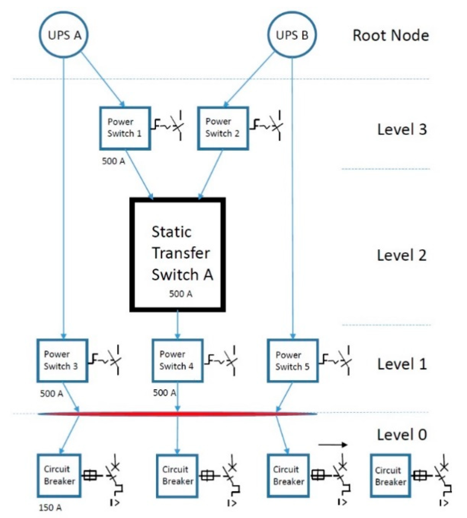
Figure 3 shows an experimental block diagram of a static transfer switch that has the task of transferring power from one UPS to another in the event of a fault or failure of the first UPS.
In the experimental block of the power supply, the two root nodes represent two redundant paths in the node diagram. On these nodes, events and alarms are associated with the program process. The node tree is used to provide more precise and transparent information on the causes and consequences. The theory of tree graphs was used, based on the fact that a tree is a type of non-directional graph in which two or more nodes are connected with exactly one path [
35,
36]. Node trees are flexible for the processing of mixed real and categorical properties. It is mandatory that data are obtained from all components. When all nodes are defined, they can be easily added and sorted. Sophisticated tree models produced by software can use historical data to perform statistical analysis and predict event probabilities. In
Figure 3, the internode (marked with a red line) is a node with information such as links and interconnections and is used anywhere where there is more than one linear path. Once the block diagram is defined for the entire technical infrastructure (
Figure 1), the tree nodes with their properties are stored in the database.
3.3. The Root Cause Method
The root cause method (RCM) follows the problem to its source [
37,
38]. RCM assumes that systems and events are dependent and may be related. An event in one part of the system causes an effect in a second part of the system and then results in an undefined alarm. An event that follows its source can be used to identify the source of the problem and its consequences and subsequent events. Different patterns of negative consequences, hidden deficiencies in the search system, and the events that led to the problem need to be explored. There is a possibility that RCM will disclose more than one cause. RCM first requires the definition of the root cause (RC). The following appropriate definitions can be used:
- -
RC is a specific cause;
- -
RCs are those that are logically identified;
- -
RCs are those that are monitored by system administrators.
The main RCM steps are as follows:
- -
Data acquisition;
- -
Graphical display of all root factors (
Figure 4);
- -
RC identification;
- -
Change proposal generation and implementation.
Once the data are acquired, graphical display of the events and root factors helps us identify the sequence of events and their connection to the circumstances. These events and current circumstances are displayed on a timeline (
Figure 4).
The events and conditions proven by facts are displayed along the full line. A graphical display of the events and root factors
- -
shows the root-cause-based explanation and causes for events;
- -
helps identify those key areas that represent weak points of system functioning;
- -
helps guarantee objectivity in cause identification;
- -
helps prove events and root factors;
- -
shows multiple cause situations and their mutual dependencies;
- -
shows the chronology of events;
- -
shows the basis for helpful changes aimed at preventing the error reappearance in the future;
- -
is efficient in helping further system design and planning.
The advantages of an event and root factor graphical display are as follows:
- -
It provides the structure for recording known facts and proof;
- -
It reveals the gaps in system knowledge through logical connections;
- -
It enables integration of other software tool results.
Once the root factors are identified, the process of root cause identification starts. The novelty of the RCM method is the use of the event cause–consequence diagram (
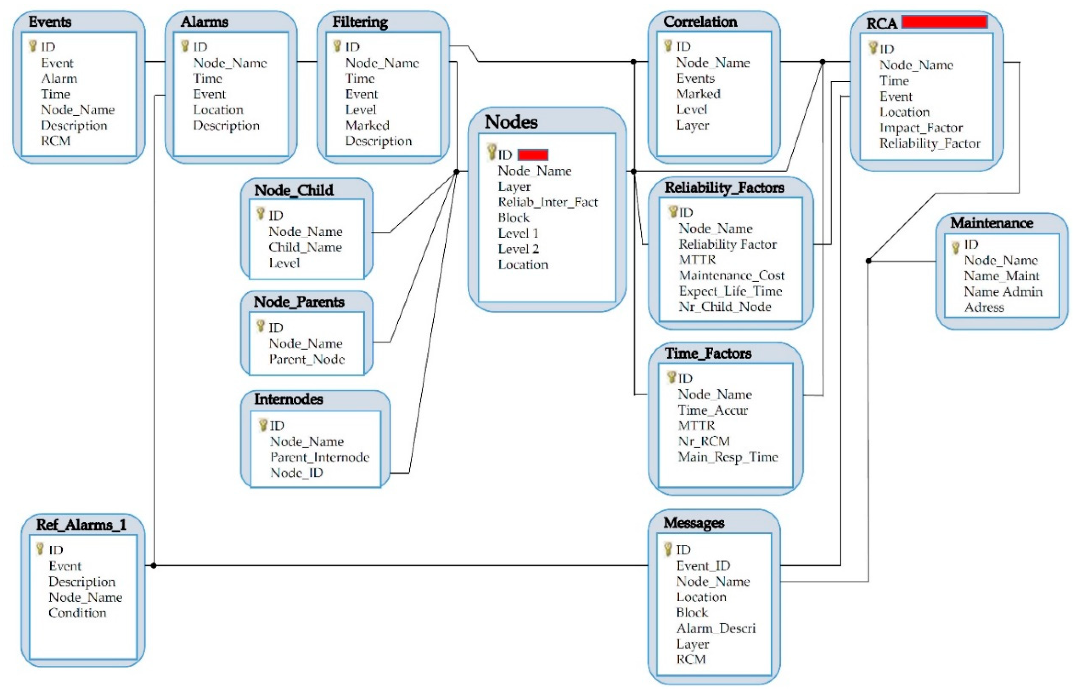
Figure 4), entity relationship diagram (
Figure 5), the node entities model (
Figure 2), and the RCM search algorithm (
Figure 6). The first diagram structures the sampling procedure, answering the question of why a certain root factor exists/appears. It is followed by a failure root diagram used for possible system failure identification. It is frequently used in the design stage and performs well when we search for possible cause relations. It requires the use of specific data with component failure probability values. Based on the block diagram described in
Section 3.3 (
Figure 3), the connections between the nodes are defined by entities and attributes for the individual node in question.
Figure 5 demonstrates the database model with connections among individual tables. The primary key in the node table is the node name and ID, which is unique for a given node and connected to most of the tables.
With RCM, a query procedure starts with a node with no child. When an internode exists as a parent of a node, all other children from the internodes can be ignored. The steps and RCM procedure were carried out using programming language SQL and a SQL server with event data, saved in the database.
Figure 6 shows the key steps of the acquired data processing. More root causes were identified due to the special rules saved with node entities: in the case when the node is the redundant power supply possibility, it always has to be considered as a root cause option.
The backward chaining method was used to find the root cause from the group of related events. RCM theory runs heuristically with experts and usually uses a manual cause-and-effect diagram to determine the reasons why there is a specific causative factor or why it happens for all possible causes and effects. Proposals for corrective actions must then address the causes that have been identified during the analysis process.
3.4. An Overview of Alternative Literature on Big Data Reducing Methods
This section provides an overview of original research and literature on the subject that was gathered through a search of the Web of Science portals.
In the big data methods, new challenges have emerged regarding the computing requirements and strategies for conducting operations management analysis. Data minimizing methods combine statistical and machine learning models, which makes them versatile in dealing with different types of data; however, these methods suffer from the weaknesses of the underlying models [
39]. In [
40], to better understand processor design decisions in the context of data analytics in data centers, comprehensive evaluations using representative data analytics workloads on representative conventional multi-core and many-core processors were conducted. After a comprehensive analysis of performance, power, and energy efficiency, the authors made the following observation: contrasting with the conventional wisdom that uses wimpy many-core processors to improve energy efficiency, brawny multi-core processors and dynamic overclocking technologies outperformed their counterparts in terms of both execution time and energy efficiency for most of the data analytics workloads in the experiments performed. In [
41], the integration and coordination of big data were required to improve the application and network performance of big data applications. While the empirical evaluation and analysis of big data can be one way of observing proposed solutions, it is often impractical or difficult to apply for several reasons, such as the expense, time consumption, and complexity. Thus, simulation tools are preferable options for performing cost-effective, scalable experimentation in a controllable, repeatable, and configurable manner.
Markov chains are stochastic models describing a sequence of events in which the probability of each event depends only on the previous state of the event. In data reduction and reconstruction using Markov Models, higher batch sizes reduce accuracy as the reconstruction does not retain the information which is present in the original dataset. Following a hybrid active/passive approach [
42], this paper introduces a family of change-detection mechanisms, differing in the required assumptions and performance. In [
43], the authors considered the scenario where the number of virtual CPUs requested by each customer job may be different, and they proposed a hierarchical stochastic modeling approach applicable to performance analysis under such a heterogeneous workload. In [
44], the authors addressed the problem of proposing and evaluating large-scale data centers to efficiently reduce bandwidth and storage for telemetry data through real-time modeling using Markov-chain-based methods. Large-scale data centers are composed of thousands of servers organized in interconnected racks to offer services to users. These data centers continuously generate large amounts of telemetry data streams (e.g., hardware utilization metrics) used for multiple purposes, including resource management and real-time analytics.
Article [
45] proposed an irregular sampling estimation method to extract the main trend of a time series, in which the Kalman filter was used to remove the noise, missing data, and outliers; then, cubic spline interpolation and averaging methods were used to reconstruct the main trend. In [
46], transport protocols such as optical packet switching and optical burst switching allowed a one-sided view of the traffic flow in the network. This resulted in disjointed and uncoordinated decision-making at each node. For effective resource planning, there is a need to consider joining distributed and centralized management, which anticipates the system’s needs and regulates the entire network using Kalman filters. In [
47], multisensor data fusion and distributed state estimation techniques that enable local processing of sensor data were the means of choice in order to minimize storage. In particular, a distributed implementation of the optimal Kalman filter was recently developed. A disadvantage of this algorithm is that the fusion center needs access to each node so as to compute a consistent state estimate, which requires full communication each time an estimate is requested.
3.5. Experimental Results of a Reduced Number of Alarms by RCM
The RCM was run on stored data collected between 2016 and 2019 and filtered by a correlation process. The data query starts at a node or a group of nodes without children. Nodes that share the same group of parents have the same internode. The procedure checks the parental status of all nodes in the possible alarm state. If the parent of the observed node is in an alarm state, the repeat loop procedure is performed in the method, checking the state of the next parent until it reaches a parent without further errors. When you follow a parental path up the tree diagram, you need to check the one redundancy path with the highest parental priority. Later, the paths of parents with lower priority factors are checked. After the use of data queries, different RCM results are possible:
- -
The root event is on the linear path in the tree node diagram with no other parent in the event
- -
having a malfunction;
- -
Multiple parents with priority values and all redundant routes are checked to define the main
- -
current event;
- -
No connected nodes with the current event;
- -
A Level 1 event can have a root cause on Level 0;
- -
The data connections of multiple line paths are checked with possible events;
- -
The priority classification of alarms due to the reliability of the node is triggered.
When managing and acquiring a great amount of data, data overwrite, data reduplication, missing transfer data, and many other related events can happen. Because of these possible events, data filtering has to be done in the selected time interval. Filtering also enables the same type of event gathered via different types of interfaces to be marked as the same event. This scenario is frequently used when the DC infrastructure is operational, because it is not possible to anticipate all events during the design stage.
During the first experiment, first the data center power supply level was simulated. The same test data were manually inserted into the database in
Table 3 and
Table 4 (“Events”).
Table 3 shows the number of alarms without using RCM, and
Table 4 shows that when it was used. The main cause was inserted as a failure of the diesel generator due to a filter failure. All nodes had an alarm event. For a more transparent presentation, the alarm nodes were grouped into parts connected to the same device or cabinets and power devices. For example, a component in the line labeled “DEG” (
Table 3 and
Table 4) refers to a diesel electric generator. The power supplies of the system cabinets are marked with “Psc 1, 2, 3”. The power distribution units are designated as “Pdu 1, 2” and they are in all IT cabinets. The “UPS A, B” labels represent uninterruptible power supplies and all components related to them. The “Cch A, B” are cooling chillers. “Psc A, B” represent power supplies of the cooling devices. The successive steps in the process from “Events” to “Alerts” were systematically derived as shown in
Table 4. The RCM inquiry procedure (
Figure 2 and
Figure 3) started with a childless node. In the event that the internode existed as the main node, all other children of the internode were ignored. Several specific causes were identified due to special rules stored with node entities. To find the root cause of a group of related events, the reverse method was used. After filtering the data, a correlation process was used to combine the associated alarm events with the same parent group. A correlation step must be performed in order to search for all related events among alarms. Correlation does not imply causation [
48,
49], which means that one alarm event does not necessarily cause another. It can only be assumed, as to the definitions, that if the events are correlated, that means that a change in one event causes a change in another node. The correlation factor in this approach is related connectivity. If there are any alarm events that have the same parents, they are grouped together, so the node path of these events is checked in the root cause analysis only once.
After linking related events to internodes, the correlation method yielded results for each part of the system, as shown in
Table 4 in the “Correlation” row.
Table 4 shows that the number of alarm events decreased.
For example, in Psc 1, 2, and 3, the system cabinets are all directly connected to power switches. They all have the same parental internal hub and the same power supply group (UPS A, B) (
Figure 3). The alarm events of these system cabinets were merged and therefore reduced to the same internal node. Therefore, due to the RCM, the alerts were carried out for the following:
- -
The diesel generator, which is also the main cause and one redundant power option;
- -
UPS A and UPS B, which were identified as a root cause because of the redundancy option;
- -
Cch A and Cch B, which have the same power source as the main network power supply.
From the number of events, it was calculated that the number of saved alarms/alerts decreased to 38%, which means that the average number of all alarms decreased by 62% (
Table 4).
Another experiment was performed on data stored in the history on messages sent to administrators. These messages contained all the information about events that had happened in the past. The event data that were stored were compared to the currently detected causes. The messages were gathered by blocks (system functional parts) and by data type in the CODESYS software. Event declarations can be sorted by individual blocks. The connections to nodes to which an event is related can be determined in the list and during event identification. The event origin (device, node, type of event) can be determined for event variables. An example of the table with event declarations and alarm statuses for the cooling cabinets is shown in
Table 5 below.
Table 6 shows an example of alarm activation areas with variables for the border regions for the cooling cabinet temperature measurement.
With the RCM running on the stored data, the number of events was decreased by ~50% for the period from 2016 to 2019 (
Table 7).
Table 7, a comparison of the total numbers of all events between 2016 and 2019, shows that when using the RCA method, the number of detected real alarms increased with increasing number of alarms (events). There were no data center downtime periods during the event collection period.


