Saturation Based Nonlinear FOPD Motion Control Algorithm Design for Autonomous Underwater Vehicle

Abstract

The application of Autonomous Underwater Vehicle (AUV) is expanding rapidly, which drives the urgent need of its autonomy improvement. Motion control system is one of the keys to improve the control and decision-making ability of AUVs. In this paper, a saturation based nonlinear fractional-order PD (FOPD) controller is proposed for AUV motion control. The proposed controller is can achieve better dynamic performance as well as robustness compared with traditional PID type controller. It also has the advantages of simple structure, easy adjustment and easy implementation. The stability of the AUV motion control system with the proposed controller is analyzed through Lyapunov method. Moreover, the controlled performance can also be adjusted to satisfy different control requirements. The outperformed dynamic control performance of AUV yaw and depth systems with the proposed controller is shown by the set-point regulation and trajectory tracking simulation examples.

1. Introduction

Autonomous Underwater Vehicle (AUV) is one of the most important research fields of marine science and technology [1,2,3]. Different from other underwater vehicles, AUV has some specific advantages. In intelligence, AUV is relatively small and has no physical connection with the mother ship, so it has certain autonomous decision-making and control capabilities. In safety, AUV can replace human beings in underwater operation, avoiding the defects of high risk factor, high strength and low efficiency of manual operation. In addition, compared with other underwater equipment, AUVs have lower manufacturing and operating costs, making it more economical and sustainable. Therefore, AUVs have broad application prospects in civil areas such as marine salvage, marine resources exploration and development, underwater engineering construction, and in some military tasks such as underwater weapon delivery and deployment, intelligence collection and investigation, anti-submarine, underwater combat, etc. [4,5,6].

With the increasing application of AUV, the requirement for its autonomy increases. One of the keys to improve the autonomy of AUVs is enhancing the dynamic performance of its motion control system. However, there are many difficulties in AUV motion control, including the strong nonlinearity and multi-degree freedom of AUV motion control system, which makes it difficult to obtain an accurate model; the ocean environment, which is complex and vulnerable to the interference of waves, currents and other unknown factors; the load and parameter perturbations; components aging or damage; and sensor noise, transmission channel delay and other unmeasurable factors, which may also affect the motion control performance.

PID controller is one of the most widely applied controllers in practical applications, as well as in underwater vehicles motion control. Until now, it still appears frequently in the underwater vehicles equipped with high precision sensors and navigation equipments. Perrier et al. designed an improved nonlinear PID and experimented on the VORTEX underwater vehicle to overcome the nonlinearity and suppress the external interference [7]. The scheme was compared experimentally with conventional PID controller. A PID controller with the shallow water wave disturbance rejection ability was applied on the ODIN underwater vehicle [8]. Refsne et al. applied a PID controller considering the effect of ocean currents on the MKII underwater vehicle [9]. Mirhosseini et al. designed a PID depth controller based on the nonlinear model of an underwater vehicle [10]. Compared with conventional PID controller, these improved PID controllers have superior abilities of suppressing specified interference and fast response. However, the dynamic control performances of AUVs with the existed PID and improved PID controllers are usually not good enough. The controller parameters are also hard to adjust in order to satisfy different control requirements.

In recent years, fractional calculus has attracted great attention in both academic and engineering fields [11,12,13,14,15,16,17]. The development of fractional-order control algorithms provides more possibilities in achieving challenging control requirements [18,19,20]. The traditional PID type controllers only have at most three parameters, namely proportional, integral and differential parameters. Except from these three parameters, fractional-order PID type controllers may have two extra parameters, namely the integral and differential orders [21]. Benefiting from these two parameters, systems controlled by FOPID type controllers are proved to be capable in achieving better transient performance as well as robustness [22,23,24,25]. A fractional sliding mode control algorithm for a fully actuated underwater vehicle subjected to the non-differentiable disturbance was proposed in [26]. Another fractional-order PI controller was also presented for REMUS AUV to improve its maneuvering precision [27]. However, the studies of this kind of controller are still limited. Further research of the stability and dynamic control performance of FOPID type controllers used on AUVs needs more exploration.

In this paper, a saturation based nonlinear fractional-order PD (FOPD) controller is proposed for the motion control system of AUVs. Compared with traditional PID type controller, the proposed controller can achieve better dynamic performance and robustness. A saturation limitation is also added to the FOPD controller to adapt to the nonlinear of the control system. In addition, the proposed controller reserves the advantages of traditional PID type controller, such as simple structure, easy tuning and easy implementation. In the simulation examples, different objective function weight pairs are presented to satisfy different kinds of control requirements. Finally, the outperformed dynamic control performance of AUV yaw and depth systems is shown by the set-point regulation and trajectory tracking examples.

The rest of this paper is organized as follows. Section 2 presents the modelling of AUV motion control system. Section 3 gives the preliminaries of fractional calculus. The controller design and stability analysis process are presented in Section 4. Section 5 shows the simulation examples of AUV yaw and depth control with the proposed controller. Finally, conclusions are drawn in Section 6.

2. Modelling of AUV

In the body coordinate, the kinetic model of an AUV can be described in a matrix form as [6]:

$$M\stackrel{·}{v}+C\left(v\right)v+D\left(v\right)v+g(ø)=\delta +\omega ,$$

(1)

where $M\in {\mathrm{R}}^{6\times 6}$ is the inertia matrix including added mass; $C\left(v\right)\in {\mathrm{R}}^{6\times 6}$ represents the Coriolis centripetal force matrix, which is is skew symmetric and can be neglected if the AUV is moving at a low speed; $D\left(v\right)\in {\mathrm{R}}^{6\times 6}$ defines the damping matrix which is definite positive; $g(ø)\in {\mathrm{R}}^{6\times 1}$ is the restoring force vector generated by gravity and buoyancy; $\delta \in {\mathrm{R}}^{6\times 1}$ defines the force vector generated by thrusters; and $\omega \in {\mathrm{R}}^{6\times 1}$ defines the disturbance vector.

The dynamic model of an AUV in the earth coordinate can be expressed as:

$$\stackrel{·}{ø}=J(ø)v,$$

(2)

where $v=[\begin{array}{cccc}u& v& w& \begin{array}{ccc}p& q& r\end{array}\end{array}{]}^T$ is the linear velocity and angular velocity in the body coordinate, $ø=[\begin{array}{cccc}x& y& z& \begin{array}{ccc}\varphi & \theta & \psi \end{array}\end{array}{]}^T$ represents the position and attitude vector in the earth coordinate, and $J(ø)\in {\mathrm{R}}^{6\times 6}$ is the transformation matrix between the body coordinate and the earth coordinate.

3. Fractional Calculus

Fractional-Order Derivative

Fractional calculus is an extension of traditional calculus. Until now, there is still no unified definition of fractional calculus. Grunwald–Letnikov, Riemann–Liouville, and Caputo definitions are used extensively in related studies. Here, we primarily introduce the Riemann–Liouville and Caputo definitions, which have been frequently applied in solving engineering and computing problems [17].

Definition 1.

[28] The α order Riemann–Liouville derivative of a function $f\left(t\right)\in C^{n+1}(\left[t_0,+\infty \right],\mathrm{R})$ is

$${}_{t_0}^L{D}_t^{\alpha }f\left(t\right)=\frac{1}{\Gamma (n-\alpha )}{\left(\frac{d}{dt}\right)}^n{\int }_{t_0}^t\frac{f\left(\tau \right)}{{(t-\tau )}^{\alpha +1-n}}d\tau ,$$

where the positive integer n satisfies $n-1<\alpha \le n$, $\Gamma (·)$ is the Gamma function defined in Appendix A, and $t_0,t$ are the lower and upper limits of the operator, respectively.

Definition 2.

[28] The α order Caputo derivative of a function $f\left(t\right)\in C^{n+1}(\left[t_0,+\infty \right],\mathrm{R})$ is defined as

$${}_{t_0}^C{D}_t^{\alpha }f\left(t\right)=\frac{1}{\Gamma (n-\alpha )}{\int }_{t_0}^t\frac{f^{\left(n\right)}\left(\tau \right)}{{(t-\tau )}^{\alpha +1-n}}d\tau ,$$

where the positive integer n satisfies $n-1<\alpha \le n$.

Remark 1.

There are some differences between Riemann–Liouville and Caputo definitions, especially in terms of their initialization [29,30,31]. However, with null initial conditions, the Laplace transforms the Riemann–Liouville and Caputo derivatives are

$$\mathcal{L}\left\{{}_{t_0}^{L,C}{D}_t^{\alpha }f\left(t\right);s\right\}=s^{\alpha }F\left(s\right).$$

That means that fractional-order systems with a steady (null) initial condition described by the Riemann–Liouville and Caputo derivative exhibit a physically coherent response for controlled systems [28]. Due to this uniform characteristic, a unified fractional-order operator ${\mathcal{D}}^{\alpha }$ is used instead of ${}_{t_0}^L{D}_t^{\alpha }$ or ${}_{t_0}^C{D}_t^{\alpha }$ throughout the remainder of this paper.

The Mittag–Leffler function is a generalization of exponential function and is an important component in the solution of fractional differential equations. A two-parameter Mittag–Leffler function can be expressed as [17]:

$$E_{a,b}\left(x\right)=\sum _{k=0}^{\infty }\frac{x^k}{\Gamma (ak+b)},$$

(3)

where $a>0,b>0$ and $x\in \mathrm{C}$. The Laplace transform of a two-parameter Mittag–Leffler function is:

$$\mathcal{L}\left\{t^{b-1}{E}_{a,b}(-\lambda t^a)\right\}=\frac{s^{a-b}}{s^a+\lambda },(\mathrm{Re}\left(s\right)>{\left|\lambda \right|}^{\frac{1}{a}}),$$

(4)

where $t\ge 0$, and $\mathrm{Re}\left(s\right)$ is the real part of s.

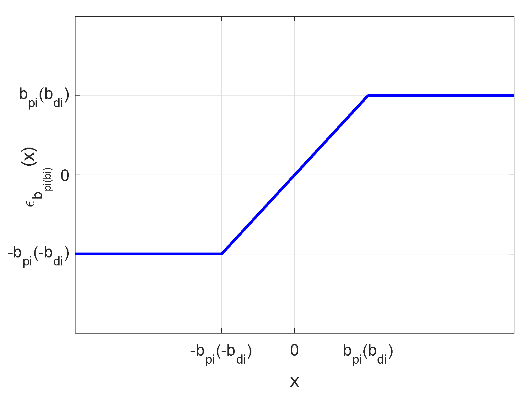
4. Saturation Based Nonlinear FOPD Controller Design

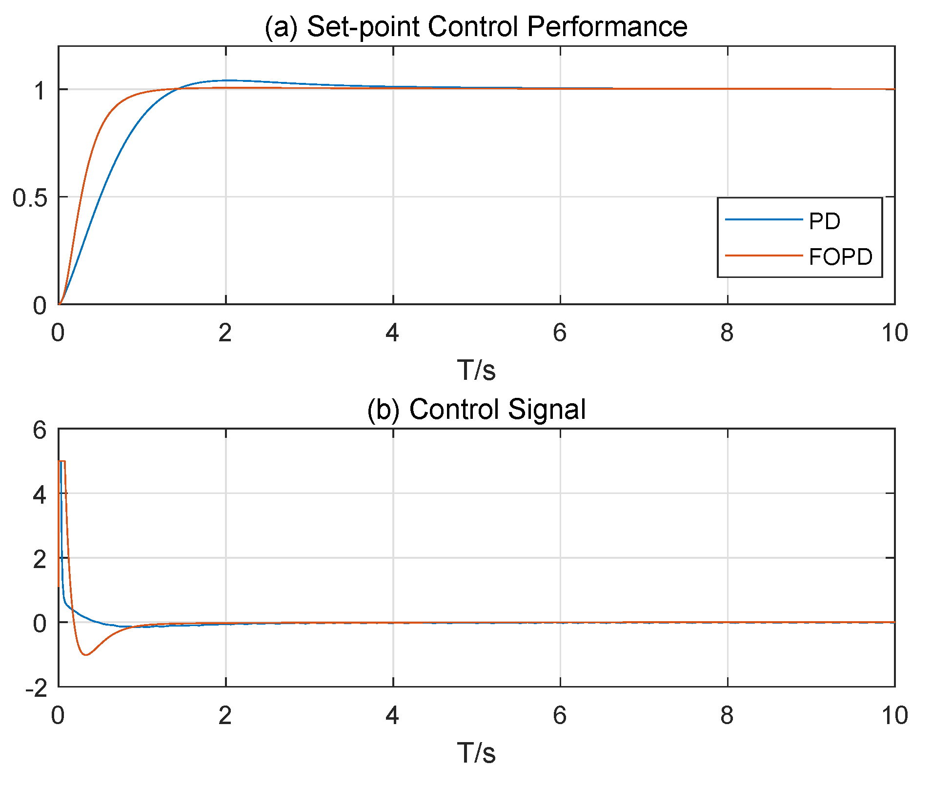
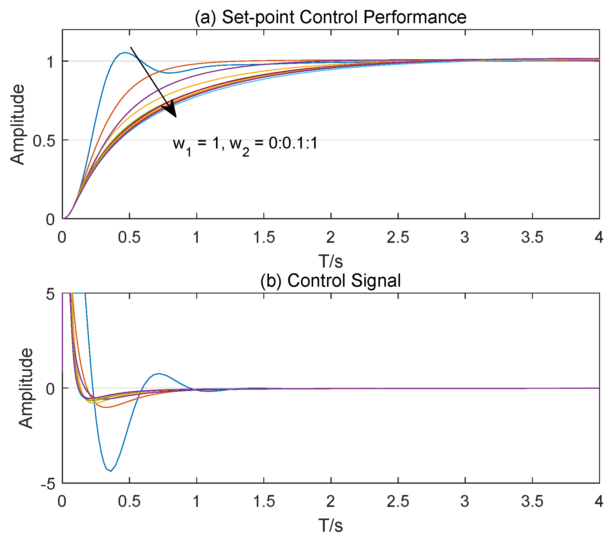
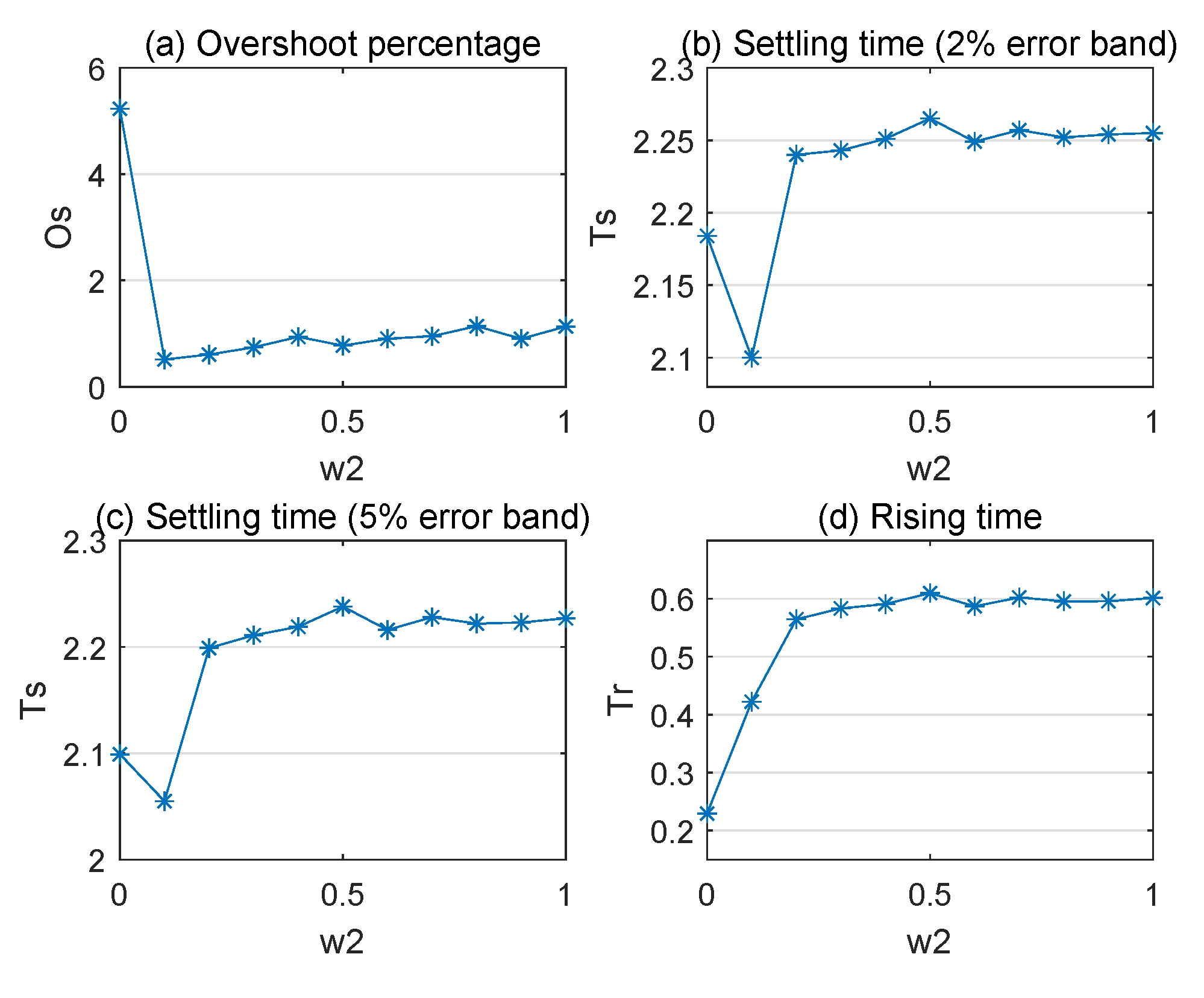
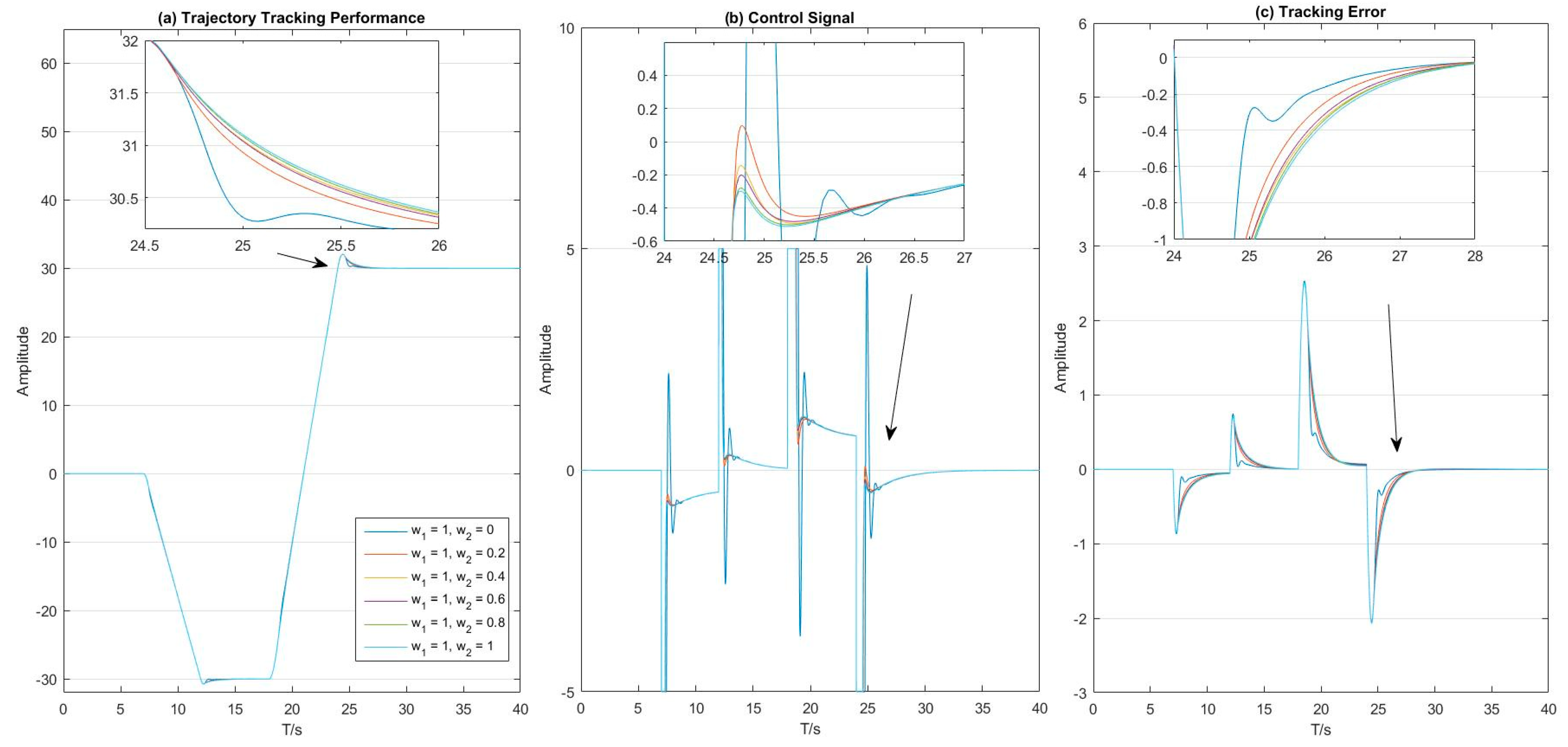
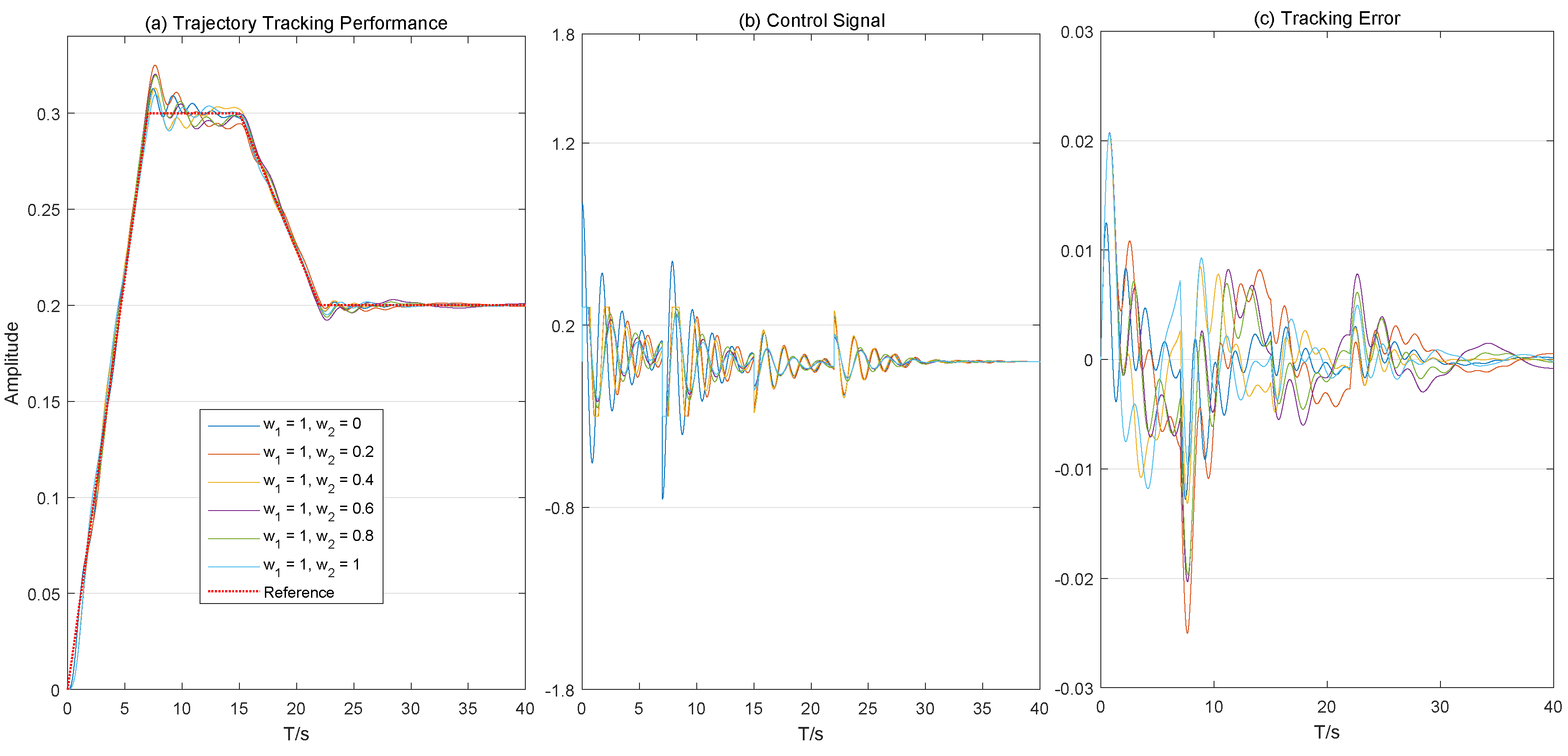
In this section, a nonlinear FOPD (FONLPD) based on saturations is proposed for the virtual closed-loop. Compared with conventional PID type controllers, FOPID type controllers have more tuning knobs, namely the integration and derivation orders, so they may provide more opportunities in improving system robustness as well as transient control performance. Consider the dynamic models in Equations (1) and (2); the FONLPD control law with gravity/buoyancy compensation can be expressed as [32]:

$$\delta =g(ø)-J(ø){\delta }_{FONLPD},$$

(5)

and

$${\delta }_{FONLPD}={\epsilon }_{{\overline{b}}_p}\left[K_{p}e\left(t\right)\right]+{\epsilon }_{{\overline{b}}_d}\left[K_d{D}^{\alpha }e\left(t\right)\right],$$

(6)

where $e\left(t\right)=ø-{ø}_d$ is the error between the reference value and actual value,

$$K_p=\left[\begin{array}{ccc}{k}_{p1}& \dots & 0\\ ⋮& \ddots & ⋮\\ 0& \cdots & k_{pn}\end{array}\right],K_d=\left[\begin{array}{ccc}{k}_{d1}& \dots & 0\\ ⋮& \ddots & ⋮\\ 0& \cdots & k_{dn}\end{array}\right],$$

are proportional and derivation parameters (diagonal, positive definite matrices), $1\le \alpha <2$ is the derivation order, $D^{\alpha }(·)$ is the fractional derivation operator, and ${\epsilon }_{{\overline{b}}_p},{\epsilon }_{{\overline{b}}_d}$ are saturation function matrices as

$$\begin{array}{c}\hfill {\epsilon }_{{\overline{b}}_p}\left[K_{p}e\left(t\right)\right]={\left[\begin{array}{c}{\epsilon }_{{\overline{b}}_{p1}}\left[k_{p1}{e}_1\left(t\right)\right],\cdots ,{\epsilon }_{{\overline{b}}_{pn}}\left[k_{pn}{e}_n\left(t\right)\right]\end{array}\right]}^T,\end{array}$$

(7)

$$\begin{array}{c}{\epsilon }_{{\overline{b}}_d}\left[K_d{D}^{\alpha }e\left(t\right)\right]={\left[\begin{array}{ccc}{\epsilon }_{{\overline{b}}_{d1}}\left[k_{d1}{D}^{\alpha }{e}_1\left(t\right)\right],& \cdots ,& {\epsilon }_{{\overline{7}b}_{dn}}\left[k_{dn}{D}^{\alpha }{e}_n\left(t\right)\right]\end{array}\right]}^T.\end{array}$$

(8)

In Equations (7) and (8), ${\epsilon }_{{\overline{b}}_{pi}}\left[k_{pi}{e}_i\left(t\right)\right]$ and ${\epsilon }_{{\overline{b}}_{di}}\left[k_{di}{D}^{\alpha }{e}_i\left(t\right)\right]$ ($i=1\dots n$) are saturation functions (seeing Figure 1) defined by

$$\begin{array}{c}\hfill {\epsilon }_{{\overline{b}}_{pi}}\left[k_{pi}{e}_i\left(t\right)\right]=\left\{\begin{array}{c}\begin{array}{c}{k}_{pi}{e}_i\left(t\right),\mathrm{if}\left|e_i\left(t\right)\right|\le w_{pi}\hfill \end{array}\hfill \\ \begin{array}{c}sign\left(e_i\left(t\right)\right){\overline{b}}_{pi},\mathrm{if}\left|e_i\left(t\right)\right|>w_{pi}\hfill \end{array}\hfill \end{array}\right.,\end{array}$$

(9)

$$\begin{array}{c}\hfill {\epsilon }_{{\overline{b}}_{di}}\left[k_{di}{D}^{\alpha }{e}_i\left(t\right)\right]=\left\{\begin{array}{c}\begin{array}{ccc}{k}_{di}{e}_i\left(t\right),& \mathrm{if}& \left|D^{\alpha }{e}_i\left(t\right)\right|\le w_{di}\end{array}\hfill \\ \begin{array}{ccc}sign\left(D^{\alpha }{e}_i\left(t\right)\right){\overline{b}}_{di},& \mathrm{if}& \left|D^{\alpha }{e}_i\left(t\right)\right|>w_{di}\end{array}\hfill \end{array}\right.,\end{array}$$

(10)

where positive constants ${\overline{b}}_{pi}$ and ${\overline{b}}_{di}$ are the bounds of saturation functions ${\epsilon }_{{\overline{b}}_{pi}}\left[k_{pi}{e}_i\left(t\right)\right]$ and ${\epsilon }_{{\overline{b}}_{di}}\left[k_{di}{D}^{\alpha }{e}_i\left(t\right)\right]$ ($i=1\dots n$), respectively, and $w_{pi}={\overline{b}}_{pi}/k_{pi}$, $w_{di}={\overline{b}}_{di}/k_{di}$. Then, we can rewrite Equations (9) and (10) as

$${\epsilon }_{{\overline{b}}_{pi}}\left[k_{pi}{e}_i\left(t\right)\right]=k_{rpi}\left(e_i\left(t\right)\right)·e_i\left(t\right),$$

(11)

$${\epsilon }_{{\overline{b}}_{di}}\left[k_{di}{D}^{\alpha }{e}_i\left(t\right)\right]=k_{rdi}\left(e_i\left(t\right)\right)·e_i\left(t\right),$$

(12)

where

$$k_{rpi}\left(e_i\left(t\right)\right)=\left\{\begin{array}{c}\begin{array}{ccc}{k}_{pi},& \mathrm{if}& \left|e_i\left(t\right)\right|\le w_{pi}\end{array}\hfill \\ \begin{array}{c}{\overline{b}}_{pi}{\left|e_i\left(t\right)\right|}^{-1},\mathrm{if}\left|e_i\left(t\right)\right|>w_{pi}\end{array}\hfill \end{array}\right.,$$

(13)

$$\begin{array}{c}\hfill k_{rdi}\left(D^{\alpha }{e}_i\left(t\right)\right)=\left\{\begin{array}{c}\begin{array}{ccc}{k}_{di},& \mathrm{if}& \left|e_i\left(t\right)\right|\le w_{di}\end{array}\hfill \\ \begin{array}{c}{\overline{b}}_{di}{\left|e_i\left(t\right)\right|}^{-1},\mathrm{if}\left|D^{\alpha }{e}_i\left(t\right)\right|>w_{di}\end{array}\hfill \end{array}\right..\end{array}$$

(14)

To analyze the stability of the system in Equation (1) under the FONLPD control law (Equation (5)), a helpful Lemma 1 is given at first.

Lemma 1

([33]). Let $x\left(t\right)\in R$ be a continuous and derivable function. Then, for any $\beta \in (0,1)$, it satisfies

$$\frac{1}{2}{D}^{\beta }{x}^2\left(t\right)\le x\left(t\right)D^{\beta }x\left(t\right).$$

In addition, when $x\left(t\right)\in R^n$ is continuous and derivable, it has

$$\frac{1}{2}{D}^{\beta }{x}^T\left(t\right)x\left(t\right)\le x^T\left(t\right)D^{\beta }x\left(t\right),\forall \beta \in (0,1).$$

The proof of Lemma 1 can be found in Appendix A.

Then, we give the stability analysis as follows.

Theorem 1.

The system in Equation (1) is asymptotically stable if the nonlinear PD control (NLPD) is designed as

$$\begin{array}{c}\hfill \delta =g(ø)-J^{\mathrm{T}}(ø)\left[K_{rp}\left(e\left(t\right)\right)e\left(t\right)+K_{rd}\left(D^{\alpha }e\left(t\right)\right)D^{\alpha }e\left(t\right)\right],\end{array}$$

(15)

where $1\le \alpha <2$,

$$K_{rp}\left(e\left(t\right)\right)=\left[\begin{array}{ccc}{k}_{rp1}\left(e_1\left(t\right)\right)& \dots & 0\\ ⋮& \ddots & ⋮\\ 0& \cdots & k_{rpn}\left(e_n\left(t\right)\right)\end{array}\right]>0,$$

$$\begin{array}{c}{K}_{rd}\left(D^{\alpha }e\left(t\right)\right)=\left[\begin{array}{ccc}{k}_{rd1}\left(D^{\alpha }{e}_1\left(t\right)\right)& \dots & 0\\ ⋮& \ddots & ⋮\\ 0& \cdots & k_{rdn}\left(D^{\alpha }{e}_n\left(t\right)\right)\end{array}\right]>0,\hfill \end{array}$$

are defined in Equations (13) and (14).

The proof of Theorem 1 can be found in Appendix A.

5. Simulations

The stability of AUV motion control system with the proposed controller is analyzed in the last section. Sine we prefer the pitch and roll angles of AUV to be close to zero in many applications, only yaw and depth motions are considered in this section [32].

Firstly, the yaw motion control performance of AUV is presented; the main features of the presented AUV can be found in [34]. To take the control performance and effect as well as energy efficiency into consideration, the controller parameters of the proposed FOPD and traditional PD controller are tuned by the following objective function F [35].

$$\begin{array}{c}\hfill F=w_1\times ITAE+w_2\times ISCO,\end{array}$$

(16)

where $ITAE={\int }_0^{\infty }t\left|e\left(t\right)\right|dt$ stands for the integrated time absolute error criterion, $ISCO={\int }_0^{\infty }{u}^2\left(t\right)dt$ stands for the control effort respectively, and $w_1,w_2$ are their weights which can help adjust the control performance. The set-point control performance comparison of the proposed nonlinear FOPD controller and a traditional nonlinear PD controller with $\delta =5$ is shown in Figure 2. The parameters ($k_p,k_d$) of traditional PD controller are ($0.9464,4.832$), ($k_p,k_d,\mu$) of FOPD controller are ($1.125,5.453,0.617$), and $w_1,w_2$ in Equation (16) are set as $1.0$. These parameters are achieved using the Nelder–Mead simplex optimization method with the objective function F [36]. It can be seen that the set-point control performance of the proposed FOPD controller is much better than traditional PD controller with smaller overshoot and rising time, which can ensure the rapidity and smoothness of the AUV yaw control performance.

Then, to show the flexibility of the proposed controller, the weight pairs $(w_1,w_2)$ are tuned to satisfy different control requirements. Because that dynamic control performance and robustness are usually more important than relatively low control signal in most control requirements, $w_1$ and $w_2$ are set to 1 and 0:0.1:1, respectively. Figure 3 shows the set-point performance comparison of different weight pairs. The corresponding evaluation indicator trends of set-point control performance, namely overshoot, settling time and rising time, are illustrated in Figure 4. Clearly, the control performance is not very satisfactory when $w_2=0$, which may be caused by the large control signal without restriction. This indicates that the ISCO criterion is necessary in the design of the proposed nonlinear PD controller. With the increase of $w_2$ from $0.1$, almost all the evaluation indicators increase sharply at first and then slightly afterwards. This example shows that the set-point regulation performance of AUV yaw system can be tuned to satisfy different control requirements.

Finally, the trajectory tracking performance of AUV yaw and depth system are shown in Figure 5 and Figure 6 with different weight pairs, respectively. The control signal of the yaw system when $w_2=0$ oscillates severely, which accords with the results in set-point control performance. Except from the control signal oscillation, all the trajectory tracking performance of AUV yaw system are quite accurate, as shown in Figure 5. However, the overshoots and settling times of the AUV depth tracking performance are relatively large when $w_2$ is quite small and decrease with the increase of $w_2$, which also accords with the results in yaw control system. Moreover, both the control signal and tracking error also decrease along with the increase of $w_2$.

6. Conclusions

This paper proposes a nonlinear FOPD controller for AUV motion control system based on saturation limitation. The proposed controller owns the advantages of improving system robustness and transient control performance, which is also easy to tune and implement. The stability of the controlled system is analyzed by Lyapunov method. The transient performance of regulation and tracking control can also be adjusted to satisfy different control requirements with the proposed controller. The simulations of both set-point regulation and trajectory tracking performance of AUV yaw and depth systems are quite satisfactory. The weights of ITAE and ISCO criteria in the optimization objective function can also be adjusted to fulfill different control requirements. With the increase of $w_2$, almost all the evaluation indicators increase sharply at first and then slightly afterwards, which means both criteria need to be taken into account. The simulation results verify the effectiveness and flexibility of the proposed control method. The future work may include other fractional-order controllers designed for AUV motion systems in order to further improve the robustness and dynamic performance of the closed-loop system.

References

1. Ge, H.; Chen, G.; Xu, G. Multi-AUV cooperative target hunting based on improved potential field in a surface water environment. Appl. Sci. 2018, 8, 973. [Google Scholar] [CrossRef]
2. Wynn, R.B.; Huvenne, V.A.; Le Bas, T.P.; Murton, B.J.; Connelly, D.P.; Bett, B.J.; Ruhl, H.A.; Morris, K.J.; Peakall, J.; Parsons, D.R.; et al. Autonomous underwater vehicles (AUVs): Their past, present and future contributions to the advancement of marine geoscience. Mar. Geol. 2014, 352, 451–468. [Google Scholar] [CrossRef]
3. Fossen, T.I.; Johansen, T.A. A survey of control allocation methods for ships and underwater vehicles. In Proceedings of the IEEE Mediterranean Conference on Control and Automation, Ancona, Italy, 28–30 June 2006. [Google Scholar]
4. Wang, J. Research on motion control of underwater vehicle. In Proceedings of the Chinese Control and Decision Conference, Taiyuan, China, 23–25 May 2012; pp. 1–6. [Google Scholar]
5. Xiang, X.; Yu, C.; Lapierre, L.; Zhang, J.; Zhang, Q. Survey on fuzzy-logic-based guidance and control of marine surface vehicles and underwater vehicles. Int. J. Fuzzy Syst. 2017, 20, 572–586. [Google Scholar] [CrossRef]
6. Cui, R.; Zhang, X.; Cui, D. Adaptive sliding-mode attitude control for autonomous underwater vehicles with input nonlinearities. Ocean. Eng. 2016, 123, 45–54. [Google Scholar] [CrossRef]
7. Perrier, M.; Canudas-De-Wit, C. Experimental comparison of PID vs. PID plus nonlinear controller for subsea robots. Auton. Robot. 1996, 3, 195–212. [Google Scholar] [CrossRef]
8. Liu, S.; Wang, D.; Poh, E.K.; Chia, C.S. Nonlinear output feedback controller design for tracking control of ODIN in wave disturbance condition. In Proceedings of the IEEE Oceans Conference, Washington, DC, USA, 17–23 September 2005. [Google Scholar]
9. Pettersen, K.Y. Output feedback control of slender body underwater vehicles with current estimation. Int. J. Control 2007, 80, 1136–1150. [Google Scholar]
10. Adhami-Mirhosseini, A.; Aguiar, A.P.; Yazdanpanah, M.J. Seabed tracking of an autonomous underwater vehicle with nonlinear output regulation. In Proceedings of the IEEE Conference on Decision & Control, Orlando, FL, USA, 12–15 December 2011. [Google Scholar]
11. Podlubny, I. Fractional-order systems and PIλDμ controllers. IEEE Trans. Autom. Control 1999, 44, 208–214. [Google Scholar] [CrossRef]
12. Oustaloup, A.; Sabatier, J.; Lanusse, P.; Malti, R.; Melchior, P.; Moreau, X.; Moze, M. An overview of the CRONE approach in system analysis, modeling and identification, observation and control. IFAC Proc. Vol. 2008, 41, 14254–14265. [Google Scholar] [CrossRef]
13. Liu, L.; Xue, D.; Zhang, S. Closed-loop time response analysis of irrational fractional-order systems with numerical Laplace transform technique. Appl. Math. Comput. 2018, 350, 122–152. [Google Scholar] [CrossRef]
14. Gao, Z. Kalman filters for continuous-time fractional-order systems involving fractional-order colored noises using tustin generating function. Int. J. Control Autom. Syst. 2018, 16, 1049–1059. [Google Scholar] [CrossRef]
15. Xue, D. Fractional-Order Control Systems Fundamentals and Numerical Implementations; De Gruyter: Berlin, Germany, 2017. [Google Scholar]
16. Liu, L.; Zhang, S.; Xue, D.; Chen, Y. General robustness analysis and robust fractional-order PD controller design for fractional-order plants. IET Control Theory Appl. 2018, 12, 1730–1736. [Google Scholar] [CrossRef]
17. Zhang, S.; Yu, Y.; Wang, H. Mittag-Leffler stability of fractional-order Hopfield neural networks. Nonlinear Anal. Hybrid Syst. 2015, 16, 104–121. [Google Scholar] [CrossRef]
18. Liu, L.; Pan, F.; Xue, D. Variable-order fuzzy fractional PID controller. ISA Trans. 2015, 55, 227–233. [Google Scholar] [CrossRef] [PubMed]
19. Zhang, S.; Yu, Y.; Wang, Q. Stability analysis of fractional-order Hopfield neural networks with discontinuous activation functions. Neurocomputing 2016, 171, 1075–1084. [Google Scholar] [CrossRef]
20. Yin, C.; Huang, X.; Chen, Y.; Dadras, S.; Zhong, S.M.; Cheng, Y. Fractional-order exponential switching technique to enhance sliding mode control. Appl. Math. Model. 2018, 44, 705–726. [Google Scholar] [CrossRef]
21. Zhang, S.; Liu, L.; Cui, X. Robust FOPID controller design for fractional-order delay systems using positive stability region analysis. Int. J. Robust Nonlinear Control 2019, 29, 5195–5212. [Google Scholar] [CrossRef]
22. Liu, L.; Zhang, S.; Xue, D.; Chen, Y. Robust stability analysis for fractional-order systems with time-delay based on finite spectrum assignment. Int. J. Robust Nonlinear Control 2019, 29, 2283–2295. [Google Scholar] [CrossRef]
23. Cheng, S.; Wei, Y.; Chen, Y.; Wang, Y.; Liang, Q. Fractional-order multivariable composite model reference adaptive control. Int. J. Adapt. Control. Signal Process. 2017, 31, 1467–1480. [Google Scholar] [CrossRef]
24. Liu, L.; Tian, S.; Xue, D.; Zhang, T.; Chen, Y. Continuous fractional-order Zero Phase Error Tracking Control. ISA Trans. 2018, 75, 226–235. [Google Scholar] [CrossRef]
25. Rosas-Jaimes, O.A.; Munoz-Hernandez, G.A.; Mino-Aguilar, G.; Castaneda-Camacho, J.; Gracios-Marin, C.A. Evaluating fractional PID control in a nonlinear MIMO model of a hydroelectric power station. Complexity 2019, 2019, 9367291. [Google Scholar] [CrossRef]
26. Muñoz-Vázquez, A.J.; Ramírez-Rodríguez, H.; Parra-Vega, V.; Sánchez-Orta, A. Fractional sliding mode control of underwater ROVs subject to non-differentiable disturbances. Int. J. Control Autom. Syst. 2017, 15, 1314–1321. [Google Scholar]
27. Talange, D.B.; Joshi, S.D.; Gaikwad, S. Control of autonomous underwater vehicle using fractional order PIλ controller. In Proceedings of the IEEE Oceans Conference, Hyderabad, India, 28–30 August 2013. [Google Scholar]
28. Podlubny, I. Fractional Differential Equations; Academic Press: London, UK, 1999. [Google Scholar]
29. Sabatier, J.; Merveillaut, M.; Malti, R.; Oustaloup, A. How to impose physically coherent initial conditions to a fractional system? Commun. Nonlinear Sci. Numer. Simul. 2010, 15, 1318–1326. [Google Scholar] [CrossRef]
30. Achar, N.; Lorenzo, C.; Hartley, T. Initialization and the Caputo fractional derivative. In Lewis Field Report; NASA John H. Glenn Research Center: Brook Park, OH, USA, 2003. [Google Scholar]
31. Aguiar, B.; González, T.; Bernal, M. A way to exploit the fractional stability domain for robust chaos suppression and synchronization via LMIs. IEEE Trans. Autom. Control 2016, 61, 2796–2807. [Google Scholar] [CrossRef]
32. Campos, E.; Chemori, A.; Creuze, V.; Torres, J.; Lozano, R. Saturation based nonlinear depth and yaw control of underwater vehicles with stability analysis and real-time experiments. Mechatronics 2017, 45, 49–59. [Google Scholar] [CrossRef]
33. Aguila-Camacho, N.; Duarte-Mermoud, M.A.; Gallegos, J.A. Lyapunov functions for fractional order systems. Commun. Nonlinear Sci. Numer. Simul. 2014, 19, 2951–2957. [Google Scholar] [CrossRef]
34. Lu, L.Y. Motion Control and Path Planning of Underwater Vehicle. Ph.D. Thesis, Yangzhou University, Yangzhou, China, 2013. [Google Scholar]
35. Das, S.; Pan, I.; Das, S.; Gupta, A. A novel fractional order fuzzy PID controller and its optimal time domain tuning based on integral performance indices. Eng. Appl. Artif. Intell. 2012, 25, 430–442. [Google Scholar] [CrossRef]
36. Barton, R.R.; Ivey, J.S. Nelder-Mead simplex modifications for simulation optimization. Manag. Sci. 1996, 42, 954–973. [Google Scholar] [CrossRef]
37. Fossen, T.I. Handbook of Marine Craft Hydrodynamics and Motion Control; John Wiley: Hoboken, NJ, USA, 2011. [Google Scholar]
Figure 1. Saturation function.
Applsci 09 04958 g001
Figure 2. Set-point control performance comparison.
Applsci 09 04958 g002
Figure 3. Set-point control performance.
Applsci 09 04958 g003
Figure 4. Control performance indicators trends.
Applsci 09 04958 g004
Figure 5. Trajectory tracking performance of AUV yaw system.
Applsci 09 04958 g005
Figure 6. Trajectory tracking performance of AUV depth system.
Applsci 09 04958 g006